OPEN ACCESS
This paper attempts to solve the current impact at the switch point of traction inverters at a low switching frequency. For this purpose, the traditional over-modulation algorithm was improved to ensure the smooth transition of the output frequency. Based on the improved algorithm, the author set up a mathematical model, which is easy to implement due to the removal of nonlinear calculation, and verified its rationality and feasibility through off-line simulation and experiment on dSPACE semi physical platform. The simulation and experimental results show that the voltage and current waveforms in the transition region were continuous and smooth, and the harmonic content of the output current was very low. Therefore, the proposed algorithm is a feasible way for signal modulation of traction inverters.
switching frequency, over-modulation, harmonic content, modulation factor
The existing modulation algorithms for traction inverters either adopt asynchronous modulation or synchronous modulation. The asynchronous modulation can realize the full-range speed control at a high switching frequency of the inverter. When the switching frequency is low, the two modulation modes are often combined, with the asynchronous modulation in the low-speed region and the synchronous modulation in the high-speed region. The mixed modulation is very likely to cause current and torque impacts at the switch point of the two modes and at the frequency switch point, reducing the comfort of passengers in the vehicle. If the impacts are severe, the converter might shut down and even suffer from damages.
The traditional solution to the impacts is to implement over-modulation, which ensures the natural transition between asynchronous modulation and square wave modulation. However, the over-modulation strategy faces high harmonic content and torque ripple, especially in the transition between over-modulation region to square wave modulation region. This is because the transition period has a few modulated wave pulses, uncertain output waveform and high waveform symmetry.
Some research has been done on the single and double modulation modes of the over-modulation strategy. For example, References (Dantzing and Ramser, 1959; Yang et al., 2017) describe a single modulation mode and apply it to the weak magnetic control of permanent magnet synchronous motor (PMSM). The application results show that the single modulation mode is simpler than the double modulation mode, solving issues like operational complexity, but output more harmonic contents than the latter. References (Sarasola et al., 2016; Guo et al., 2016) compare the two modulation modes in details, without giving a better solution.
This paper optimizes the traditional over-modulation algorithm to reduce the harmonic content in the output current and reduce the output torque ripple of traction inverters. The remainder of this paper is organized as follows: Section 2 describes the improvement of the over-modulation algorithm and establishes a model based on the improved algorithm; Section 3 verifies the proposed model through experiments; Section 4 wraps up this paper with some meaningful conclusions.
2.1. Improvement of over-modulation algorithm
In the transition between over-modulation region to square wave region, the number of output pulses is uncertain due to the randomness of the output waveform, despite the lack of current impact in this period. In addition, the output current is rich in harmonic contents and subjected to oscillation. If the vehicle runs for a long time in this period, the protective measure may fail to work (Zufferey et al., 2016; Liu et al., 2017). Therefore, this paper improves the over-modulation algorithm based on synchronous modulation (Zhao et al., 2017):
$m = \frac { u _ { \mathrm { out } } } { u _ { \mathrm { six } } }$ (1)
where m is the modulation factor; uout is the space voltage vector (the maximum uout is $\frac { \sqrt { 3 } } { 3 } u _ { d c }$for asynchronous modulation); $u _ { s i x } = \frac { 2 } { \pi } u _ { d c }$ is the output fundamental voltage amplitude of 6-pulse inverter, its value is $\frac { 2 } { \pi } u _ { d c }$. Then, the three-phase voltage outputs U, V and W of inverter can be expressed as:
$\left\{ \begin{array} { l } { u _ { u } = k * \sin \theta } \\ { u _ { v } = k * \sin \left( \theta - \frac { 2 } { 3 } \pi \right) } \\ { u _ { w } = k * \sin \left( \theta + \frac { 2 } { 3 } \pi \right) } \end{array} \right.$ (2)
$k = 1.1026 * m * \frac { 2 } { \pi } * u _ { \mathrm { dc } }$ (3)
where ua, ub and uc are the three-phase voltage outputs; $\theta $is the position angle of stator flux linkage; k is the three-phase voltage amplitude. The value of the three-phase voltage can be derived as:
$\left\{ \begin{array} { l } { u _ { u } ^ { * } = u _ { u } / u _ { \mathrm { dc } } } \\ { u _ { v } ^ { * } = u _ { v } / u _ { \mathrm { dc } } } \\ { u _ { w } ^ { * } = u _ { w } / u _ { \mathrm { dc } } } \end{array} \right.$ (4)
$u _ { u v w } ^ { * } = \left[ u _ { u } ^ { * } , u _ { v } ^ { * } , u _ { w } ^ { * } \right]$ (5)
where $u _ { u v w } ^ { * }$ is the per-unit value set of three-phase voltage. The relationship between the three-phase voltage value and the sector is shown in Figure 1 below.
Figure 1. The relationship between the three-phase output voltage and the sector.
The action time of space voltage vectors can be further simplified as:
$\left\{ \begin{array} { l } { t _ { 1 } = T _ { \mathrm { s } } * \left[ \max \left( u _ { u v w } ^ { * } \right) - \operatorname { mid } \left( u _ { \text {unw} } ^ { * } \right) \right] } \\ { t _ { 2 } = T _ { \mathrm { s } } * \left[ \operatorname { mid } \left( u _ { u v v } ^ { * } \right) - \min \left( u _ { u v v } ^ { * } \right) \right] } \\ { t _ { 0 } = T _ { \mathrm { s } } - t _ { 1 } - t _ { 2 } } \end{array} \right.$ (6)
where $t _ { 0 } , t _ { 1 }$ and $t _ { 2 }$ are the action time of the zero vector and its adjacent vectors; Ts is the action time of space voltage vector.
In this way, the traditional over-modulation algorithm (double modulation mode) is simplified, cutting down the computing complexity and the harmonic content in over-modulation region. The simplification makes it easier to modify the mathematical model of action time, and smooths the modulation wave. Compared with the single and double modulation mode, the simplified over-modulation strategy achieves a very low harmonic content.
2.2. Optimization of the transition between over-modulation region to square wave region
When the traditional over-modulation algorithm is adopted for traction inverters, the current in the transition between over-modulation region to square wave region will oscillate due to the uncertain number of output pulses and the asymmetry of the waveform. If the vehicle runs for a long time in this period, the passengers will feel uncomfortable under the severe vibrations of the wagon. To reduce the current oscillation, it is necessary to optimize the number of pulses and the asymmetrical waveform in the transition period. By contrast, there is almost no current impact at the switch point between the three-frequency region and square wave region of the synchronous modulation.
Here, the transition period is optimized by the three-frequency Fourier decomposition of the synchronous modulation below:
$u _ { \mathrm { A } } = \sum _ { n = 1 } ^ { \infty } \left[ b _ { \mathrm { n } } \sin \left( n \omega _ { 1 } t \right) \right]$ (7)
where $b _ { n } = \frac { 2 } { \pi } \int _ { 0 } ^ { \pi } u _ { a } ( t ) \sin \left( n \omega _ { 1 } t \right) ; \omega _ { 1 }$ is the fundamental angular frequency. Note that b1 is the fundamental voltage amplitude Um1:
$U _ { \mathrm { m } 1 } = \frac { 2 U _ { \mathrm { d } } } { \pi } \left[ 1 - 2 \sin \frac { \beta } { 2 } \right]$ (8)
Let β be the pulse width. Then, the relationship between b1 and β can be expressed as:
$\beta = 2 \arcsin \left[ \frac { 1 - \pi U _ { \mathrm { s } } / \left( 2 U _ { \mathrm { d } } \right) } { 2 } \right]$ (9)
Through the above optimization, the output current will oscillate less violently when the inverter enters the transition period after the output frequency reaches the set threshold.
2.3. Simulation model based on the improved over-modulation algorithm
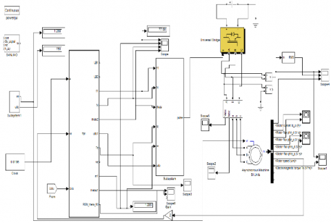
Based on the above optimized algorithm, an over-modulation simulation model (Figure 2) was compiled in M language on Matlab/Simulink, and verified through simulation experiment (Masrom et al., 2015).
To facilitate the observation and debugging of the waveform, the control algorithm was divided into three parts, namely, the module based on the improved algorithm, the module of the action time and PWM generation, and the module of the inverter and the asynchronous motor.
Figure 2. The established simulation model
Figure 3. The module of the action time and pulse-wave modulation (PWM) generation
3.1. Matlab simulation
(1) The transition from linear modulation region to over-modulation region
The simulation results on the transition from linear region to over-modulation region are as follows: the output frequency f= 0~100Hz, the modulation coefficient m=0~1, and the waveform simulated by the improved over-modulation algorithm is shown in Figures 4 and 5 below.
Figure 4. Simulation waveform of three-phase modulation and sector
Figure 5. Simulation waveform of output voltages $u _ { \alpha }$ and $u _ { \beta }$
Figures 4 and 5 are respectively the simulation waveforms of three-phase modulation and output voltages
and . It can be seen that the improved algorithm eliminated the sector determination and the regional division of the traditional algorithm, thereby reducing the computing load and smoothing the waveform transition.Figure 6. Simulation action time of space voltage vectors
Figure 6 presents the space voltage vector action time of the improved algorithm. Obviously, the time waveform was continuous and smooth from linear modulation region to over-modulation region.
Figure 7. Simulation waveform of Ia and its harmonic content
As shown in Figure 7, the simulation waveform of Ia was continuous and smooth from linear modulation region to over-modulation region, and the output current oscillated slightly. However, there was an oscillation in the transition to square wave region. In addition to the improved algorithm, the excellent simulation results in the transition from linear modulation region to over-modulation region is attributable to the many number of pulses, symmetric waveform and fixed pulse width in this transition period. The output waveform in this transition remains stable despite the increase or decrease in the number of pulses.
(2) The transition from over-modulation region to square wave region
Compared with that from linear modulation region to over-modulation region, the transition from over-modulation region to square wave region has a few pulses and fluctuation on both sides of each pulse, which affects the stability of the output waveform. Without proper improvement, the vehicle operation may not be stable in this period.
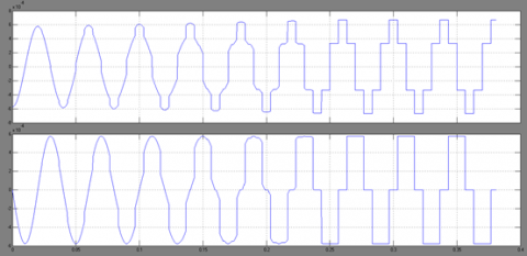
The simulation results on this transition are as follows: the output frequency f= 50~100Hz, the modulation coefficient m=0.9069~1, and the waveform simulated by the improved over-modulation algorithm is shown in Figures 8 and 9 below.
Figure 8. Transition from over-modulation region to three-frequency division region
Figure 9. Transition from three-frequency division region to square wave region
In Figures 8 and 9, the three waves respectively depict the output voltage, the root-mean-square (RMS) of the output voltage, and the instantaneous value of U-phase output current. It is clear that the output current waveform was smooth without oscillation. The results show that the optimization ensures the proportional growth of the output frequency and the carrier frequency, guarantees the symmetry of the output waveform, and suppresses the harmonic content.
Through the above analysis of the simulation results, it can be seen that the improved over-modulation algorithm outperforms the traditional algorithm in transition smoothness, the harmonic content of output current and the current oscillation.
3.2. Experiment on dSPACE semi-physical platform
The proposed method was further verified through an experiment on the dSPACE semi-physical platform. The hardware of the experiment includes a metro control cabinet, a loop test bench in-built with dSPACE hardware, a DL850 oscilloscope, and a laptop. The popular TMS320F28335 series chip was adopted for chassis control. In terms of software, the dSPACE metro 1C4M control cabinet and motor model was selected for the semi-physical platform, the communication software for RS485 serial communication interface was employed and the process variable parameters and waveform were monitored in real time by self-designed software. The software flow chart is shown below.
Figure 10. The flow chart of the improved algorithm
Before the experiment, the voltage and rated power of the platform were set to 1,500V and 180kW, respectively, while the rated voltage and rated frequency of the asynchronous motor were set to 1,100V and 50Hz, respectively. The motor has two poles and adopts vector control. The test motor and the auxiliary motor mutually back up each other. The test motor frequency changed from 0~60Hz. The experimental waveforms are shown in Figures 11 and 12, where 40Hz and 60Hz respectively mark the entry to the over-modulation region and the square wave region.
Figure 11. Transition from over-modulation region to three-frequency division region
Figure 12. Transition from three-frequency division region to square wave region
Figures 11 and 12 display the voltage and current waveforms the transition from over-modulation region to three-frequency division region and that from three-frequency division region to square wave region, respectively. It can be seen that the improved algorithm achieved smooth waveforms and low harmonic content, which agree well with the simulation results. Thus, the experiment further validates the feasibility of the proposed method.
This paper puts forward an improved over-modulation algorithm for traction inverters, with the aim to overcome current oscillation in the transition region. The improved algorithm simplifies the computation of the original algorithm. Based on the improved algorithm, the author set up a mathematical model, which is easy to implement due to the removal of nonlinear calculation, and verified its rationality and feasibility through off-line simulation and experiment on dSPACE semi physical platform. The simulation and experimental results show that the voltage and current waveforms in the transition region were continuous and smooth, and the harmonic content of the output current was very low. Therefore, the proposed algorithm is a feasible way for signal modulation of traction inverters.
This work is financially supported by Dr scientific research fund of Liaoning Province (No. 20170520229, 20180550499), and Social Science planning fund of Liaoning Province (L18BGL018, 2018lslktyb-016).
Dantzig G. B., Ramser J. H. (1959). The truck dispatching problem. Management Science, Vol. 6, No. 1, pp. 80-91. https://doi.org/10.1287/mnsc.6.1.80
Guo Y., Cheng J., Ji J. (2016). Robust dynamic vehicle routing optimization with time windows. advances in swarm intelligence. Springer International Publishing. https://doi.org/10.1007/978-3-319-41009-8_4
Liu J., Wu C., Wang Z., Wu L. (2017). Reliable filter design for sensor networks in the type-2 fuzzy framework. IEEE Transactions on Industrial Informatics, Vol. 13, No. 4, pp. 1742-1752. https://doi.org/10.1109/TII.2017.2654323
Masrom S., Abidin S. Z. Z., Omar N. (2015). Dynamic parameterization of the particle swarm optimization and genetic algorithm hybrids for vehicle routing problem with time window. International Journal of Hybrid Intelligent Systems, Vol. 12, No. 1, pp. 13-25.
Sarasola B., Doerner K. F., Schmid V. (2016). Variable neighborhood search for the stochastic and dynamic vehicle routing problem. Annals of Operations Research, Vol. 236, No. 2 pp. 425-461. https://doi.org/10.1007/s10479-015-1949-7
Yang Z., Osta J. P. V., Veen B. V. (2017). Dynamic vehicle routing with time windows in theory and practice. Natural Computing, Vol. 16, No. 1, pp. 119-134. https://doi.org/10.1007/s11047-016-9550-9
Zhao Y., Shen Y., Bernard A., Cachard C., Liebgott H. (2017). Evaluation and comparison of current biopsy needle localization and tracking methods using 3D ultrasound. Ultrasonics, Vol. 73, pp. 206-220. https://doi.org/10.1016/j.ultras.2016.09.006
Zufferey N., Cho B. Y., Glardon R. (2016). Dynamic multi-trip vehicle routing with unusual time-windows for the pick-up of blood samples and delivery of medical material. International Conference on Operations Research and Enterprise Systems, pp. 366-372.