OPEN ACCESS
An improved PSO algorithm is proposed. The algorithm improves the particle swarm optimization algorithm that has been used to solve parallel machine scheduling problem, so as to better solve the scheduling of multi-time, multi-variety and variable-batch parallel machine scheduling. The crossover operation in genetic algorithm and PSO algorithm are mixed, and different particles are cross-operated, which increases the ability of particle searching for other new positions in the space, and avoids the particle swarm falling into local optimum prematurely. In order to increase the efficiency of the distance search, we use the idea of half - searching in the searching algorithm, which further improve the scheduling efficiency of the problem and the algorithm is implemented in MATLAB.
multi-time, multi-variety, variable batch, parallel machine scheduling, improved particle swarm optimization algorithm
The scheduling problem of multi-time, multi-variety, variable batch parallel machines is an important problem in production scheduling, and it is a key link in computer integrated manufacturing system. It is widely used in the assembly line of electronic products.
The research of assembly line scheduling technology at home and abroad began around 1990s. The research on assembly scheduling strategy and control method is biased towards the flexible production line of operators using automation equipment (Song et al., 2008; Rezazadeh et al., 2011; Aghajani et al., 2014; Yu et al., 2014; Siemiatkowski & Przybylski, 2007; Book & Karp Richard, 2014; Meller & Deshazo, 2011; Liu et al., 2013; Azadeh et al., 2012). It is difficult to apply the research results to the assembly scheduling of multi-variety variable batches with changing production time, which is difficult to apply to the assembly of manipulators. Aiming at the assembly work environment of complex products, the paper (Roshani & Gigli, 2016) puts forward a scheduling strategy and control method based on Petri net specification to standardize assemble production process flow and control based on key process points. The paper proposes a method for scheduling complex products with constraints between working procedures, and studies the scheduling strategy of many varieties under the condition of various workshops. In the paper, a heuristic algorithm with working position constraint is proposed and the strategy of segmented optimization is proposed. When solving the parallel machine scheduling problem considering production time, the branch and bound method, artificial intelligence method, neural network method, genetic algorithm and simulated annealing method are applied to solve the parallel scheduling problem of unit production line in the paper. However, the above research results still exist the following problems. The first one is it mainly focus on the research of scheduling, which is lack of research on dynamic scheduling method for changing production time and batch in discrete assembly process. The second one is it mainly focuses on the objective function, whose production cost is the least, and lacks the research on the target function of the number of multi-time tardiness. The third one is it mainly focused on the operator for the production line of human resources and not consider the manipulator instead of the operator of the full automated production line research, because the manipulators appear in recent years. It is a blank to study the scheduling problem of manipulator production line in parallel production line with multiple varieties and variable batches.
Aiming at the above problems, this paper takes the electronic product assembly parallel manipulator production line as the research object, establishes the scheduling model with the target of tardiness, and proposes an improved particle swarm optimization algorithm. The model and algorithm mentioned above are compared and applied to verify. Finally, the assembly execution result with preparation time, multi-time, multi-variety and variable batch products which is orderly, controllable and efficient is realized (Shidpour et al., 2014; Akbari et al., 2013; Yu et al., 2014; Liu et al., 2012; Boulif & Atif, 2006; Filho & Tiberti, 2006; Defersha & Chen, 2008; Arkat et al., 2011).
There are i products, t period and multiple channels that accomplish the same functionality whose orders are $Q _ { i t }$ and $\mathrm { K }$ . The processing speed of i product at each multiple channelis $o _ { i k } ,$ multiple channel $k$ is capable of processing all products without a priority level for all products. Product $i , i \in I = \{ 1,2 , \ldots i \} ,$ multiple channel, $l \in K = \{ 1,2 , \ldots k \} ,$ time frame $\mathrm { t } , t \in \{ 1,2 , \ldots T \} .$ The production takt of product $j$ in each multiple channel is $o _ { i k }$ . The delivery date of the workpiece is $\mathrm { T }$ . Product group can be processed in different multichanel batches, but with minimum batch limits All product groups are ready at zero time. By optimizing the order batch and the the the the the the the the the the production schetuling stheme on each multiple channel after batching, the tota tardiness of each time period is minimized.
Scheduling model of parallel machine
When t=1:
${{\Delta }_{i1}}=\left\{ \begin{align} & {{Q}_{i1}}-\sum\limits_{k=1}^{{{K}_{1}}}{P_{i1}^{{{k}_{1}}}\begin{matrix} {} & \begin{matrix} \begin{matrix} \begin{matrix} {} \\\end{matrix} \\\end{matrix} \\\end{matrix}{{Q}_{i1}}-\sum\limits_{{{k}_{1}}=1}^{{{K}_{1}}}{P_{i1}^{{{k}_{1}}}}>0 & {} & {} \\\end{matrix}} \\ & 0\begin{matrix} {} & {} & \begin{matrix} {} \\\end{matrix}\begin{matrix} \begin{matrix} {} \\\end{matrix}\begin{matrix} {} \\\end{matrix}\begin{matrix} {} \\\end{matrix}\begin{matrix} {} \\\end{matrix} \\\end{matrix} & {{Q}_{i1}}-\sum\limits_{{{k}_{1}}=1}^{{{K}_{1}}}{P_{i1}^{{{k}_{1}}}}\le 0 \\\end{matrix} \\ \end{align} \right.$ (1)
$\Delta _{i1}^{-}=\left\{ \begin{align} & \sum\limits_{k=1}^{{{K}_{1}}}{P_{i1}^{{{k}_{1}}}-{{Q}_{i1}}\begin{matrix} {} & {} & {} & \sum\limits_{k=1}^{{{K}_{1}}}{P_{i1}^{{{k}_{1}}}-{{Q}_{i1}}}>0 \\\end{matrix}} \\ & 0\begin{matrix} {} & {} & {} & \begin{matrix} {} \\\end{matrix}\begin{matrix} {} \\\end{matrix}\begin{matrix} {} \\\end{matrix}\begin{matrix} {} \\\end{matrix}\begin{matrix} {} \\\end{matrix}\begin{matrix} {} \\\end{matrix}\begin{matrix} {} \\\end{matrix}\begin{matrix} {} \\\end{matrix}\sum\limits_{k=1}^{{{K}_{1}}}{P_{i1}^{{{k}_{1}}}-{{Q}_{i1}}}\le 0 \\\end{matrix} \\ \end{align} \right.$ (2)
t=2:
${{\Delta }_{i2}}=\left\{ \begin{align} & {{Q}_{i2}}-(\sum\limits_{{{k}_{1}}=1}^{{{K}_{1}}}{P_{i2}^{k}+\Delta _{i1}^{-})\begin{matrix} {} & {{Q}_{i2}}-(\sum\limits_{{{k}_{1}}=1}^{{{K}_{1}}}{P_{i2}^{k}+\Delta _{i1}^{-})}>0 & {} & {} \\\end{matrix}} \\ & 0\begin{matrix} {} \\\end{matrix}\begin{matrix} {} \\\end{matrix}\begin{matrix} {} \\\end{matrix}\begin{matrix} {} \\\end{matrix}\begin{matrix} {} \\\end{matrix}\begin{matrix} {} \\\end{matrix}\begin{matrix} {} \\\end{matrix}\begin{matrix} {} \\\end{matrix}\begin{matrix} {} & {} & {} & {{Q}_{i2}}-(\sum\limits_{{{k}_{1}}=1}^{{{K}_{1}}}{P_{i2}^{k}+\Delta _{i1}^{-})}\le 0 \\\end{matrix} \\ \end{align} \right.$ (3)
$\Delta _{i2}^{-}=\left\{ \begin{align} & (\sum\limits_{{{k}_{1}}=1}^{{{K}_{1}}}{P_{i1}^{{{k}_{1}}}+\Delta _{i1}^{-})-{{Q}_{i2}}\begin{matrix} {} & {} & {} & (\sum\limits_{{{k}_{1}}=1}^{{{K}_{1}}}{P_{i1}^{{{k}_{1}}}+\Delta _{i1}^{-})-{{Q}_{i2}}}>0 \\\end{matrix}} \\ & 0\begin{matrix} {} \\\end{matrix}\begin{matrix} {} \\\end{matrix}\begin{matrix} {} \\\end{matrix}\begin{matrix} {} \\\end{matrix}\begin{matrix} {} \\\end{matrix}\begin{matrix} {} \\\end{matrix}\begin{matrix} {} \\\end{matrix}\begin{matrix} {} \\\end{matrix}\begin{matrix} {} \\\end{matrix}\begin{matrix} {} \\\end{matrix}\begin{matrix} {} \\\end{matrix}\begin{matrix} {} \\\end{matrix}\begin{matrix} {} \\\end{matrix}\begin{matrix} {} & {} & {} & (\sum\limits_{{{k}_{1}}=1}^{{{K}_{1}}}{P_{i1}^{{{k}_{1}}}+\Delta _{i1}^{-})-{{Q}_{i2}}}\le 0 \\\end{matrix} \\ \end{align} \right.$ (4)
t=t:
${{\Delta }_{it}}=\left\{ \begin{align} & {{Q}_{it}}-(\sum\limits_{{{k}_{1}}=1}^{{{K}_{1}}}{P_{it}^{{{k}_{1}}}+\Delta _{i(t-1)}^{-})\begin{matrix} {} & {{Q}_{it}}-(\sum\limits_{{{k}_{1}}=1}^{{{K}_{1}}}{P_{it}^{{{k}_{1}}}+\Delta _{i(t-1)}^{-})}>0 & {} & {} \\\end{matrix}} \\ & 0\begin{matrix} {} \\\end{matrix}\begin{matrix} {} \\\end{matrix}\begin{matrix} {} \\\end{matrix}\begin{matrix} {} \\\end{matrix}\begin{matrix} {} \\\end{matrix}\begin{matrix} {} \\\end{matrix}\begin{matrix} {} \\\end{matrix}\begin{matrix} {} \\\end{matrix}\begin{matrix} {} \\\end{matrix}\begin{matrix} {} & {} & {} & {{Q}_{it}}-\sum\limits_{{{k}_{1}}=1}^{{{K}_{1}}}{P_{it}^{{{k}_{1}}}+\Delta _{i(t-1)}^{-})}\le 0 \\\end{matrix} \\ \end{align} \right.$ (5)
$\Delta _{it}^{-}=\left\{ \begin{align} & (\sum\limits_{{{k}_{1}}=1}^{{{K}_{1}}}{P_{it}^{{{k}_{1}}}+\Delta _{i(t-1)}^{-})-{{Q}_{it}}\begin{matrix} {} & {} & {} & \sum\limits_{{{k}_{1}}=1}^{{{K}_{1}}}{P_{it}^{{{k}_{1}}}+\Delta _{i(t-1)}^{-})-{{Q}_{it}}}>0 \\\end{matrix}} \\ & 0\begin{matrix} {} \\\end{matrix}\begin{matrix} {} \\\end{matrix}\begin{matrix} {} \\\end{matrix}\begin{matrix} {} \\\end{matrix}\begin{matrix} {} \\\end{matrix}\begin{matrix} {} \\\end{matrix}\begin{matrix} {} \\\end{matrix}\begin{matrix} {} \\\end{matrix}\begin{matrix} {} \\\end{matrix}\begin{matrix} {} \\\end{matrix}\begin{matrix} {} \\\end{matrix}\begin{matrix} {} \\\end{matrix}\begin{matrix} {} \\\end{matrix}\begin{matrix} {} \\\end{matrix}\begin{matrix} {} \\\end{matrix}\begin{matrix} {} & {} & {} & (\sum\limits_{{{k}_{1}}=1}^{K_{1}^{{}}}{P_{it}^{{{k}_{1}}}+\Delta _{i(t-1)}^{-})-{{Q}_{it}}}\le 0 \\\end{matrix} \\ \end{align} \right.$ (6)
t=T:
${{\Delta }_{iT}}=\left\{ \begin{align} & {{Q}_{iT}}-(\sum\limits_{{{k}_{1}}=1}^{{{K}_{1}}}{P_{iT}^{{{k}_{1}}}+\Delta _{i(T-1)}^{-})\begin{matrix} {} & {{Q}_{iT}}-(\sum\limits_{k=1}^{{{K}_{1}}}{P_{iT}^{{{k}_{1}}}+\Delta _{i(T-1)}^{-})}>0 & {} & {} \\\end{matrix}} \\ & 0\begin{matrix} {} \\\end{matrix}\begin{matrix} {} \\\end{matrix}\begin{matrix} {} \\\end{matrix}\begin{matrix} {} \\\end{matrix}\begin{matrix} {} \\\end{matrix}\begin{matrix} {} \\\end{matrix}\begin{matrix} {} \\\end{matrix}\begin{matrix} {} \\\end{matrix}\begin{matrix} {} \\\end{matrix}\begin{matrix} {} \\\end{matrix}\begin{matrix} {} \\\end{matrix}\begin{matrix} {} & {} & {} & {{Q}_{iT}}-(\sum\limits_{k=1}^{{{K}_{1}}}{P_{iT}^{{{k}_{1}}}+\Delta _{i(T-1)}^{-})}\le 0 \\\end{matrix} \\ \end{align} \right.$ (7)
$\Delta _{iT}^{-}=\left\{ \begin{align} & (\sum\limits_{k=1}^{{{K}_{1}}}{P_{iT}^{{{k}_{1}}}+\Delta _{i(T-1)}^{-})-{{Q}_{iT}}\begin{matrix} {} & {} & {} & (\sum\limits_{k=1}^{{{K}_{1}}}{P_{iT}^{{{k}_{1}}}+\Delta _{i(T-1)}^{-})-{{Q}_{iT}}}>0 \\\end{matrix}} \\ & 0\begin{matrix} {} \\\end{matrix}\begin{matrix} {} \\\end{matrix}\begin{matrix} {} \\\end{matrix}\begin{matrix} {} \\\end{matrix}\begin{matrix} {} \\\end{matrix}\begin{matrix} {} \\\end{matrix}\begin{matrix} {} \\\end{matrix}\begin{matrix} {} \\\end{matrix}\begin{matrix} {} \\\end{matrix}\begin{matrix} {} \\\end{matrix}\begin{matrix} {} \\\end{matrix}\begin{matrix} {} \\\end{matrix}\begin{matrix} {} \\\end{matrix}\begin{matrix} {} \\\end{matrix}\begin{matrix} {} \\\end{matrix}\begin{matrix} {} \\\end{matrix}\begin{matrix} {} & {} & {} & (\sum\limits_{k=1}^{{{K}_{1}}}{P_{iT}^{{{k}_{1}}}+\Delta _{i(T-1)}^{-})-{{Q}_{iT}}}\le 0 \\\end{matrix} \\ \end{align} \right.$ (8)
Among them, a represents the change preparation time for a single operator, and Ht represents t time period. Bi represents minimum batches of the i product. rk represents the number of operators in the k multichannel production line. skj represents the number of the k multichannel production lines and the quantity of equipment in the j workplace. $X _ { i k } ^ { t }$ represents that the i products are arranged in k1 production lines at t time frame as 1, otherwise 0. $P _ { i t } ^ { k _ { 1 } }$ represents the number of the i products in the k1 multichannel production line at t time frame. $\Delta _ { i t }$ represents the number of tardiness for the i product at t time frame. $\Delta _ { \overline {i t} }$ represents the remaining quantity of the i product at t time frame.
The formula (1) is a piecewise function representing the tardiness quantity for the first time period. When the quantity of the actual production of the product is greater than the quantity of the order, the number of tardiness is 0, otherwise the amount of tardiness is $\Delta _ { i 1 }$. The formula (2) is also a piecewise function representing the remaining quantity in the first period. When the actual number of products produced in that stage is greater than the order number, the remaining quantity is $\Delta _ { i 1 } ^ { - }$, otherwise the amount of tardiness is 0. $\Delta _ { i 1 }$ and $\Delta _ { i 1 } ^ { - }$ are positive integers. The remaining quantity of the first stage is positive, which indicates that the first stage is overcapacity, and the remaining quantity of the first stage is actually a part of the order from other stages except the first stage. The formula (3), (5) and (7) represent the number of tardiness in the second, t, and T stages in the piecewise function. The formula (4), (6) and (8) represent the remaining quantity in the second, t, and T stages in the piecewise function. In the case of non-permitted delay delivery, The formula 3 indicates that the tardiness of the second phase is the number of orders in the second phase minus the remaining amount of the first phase and then minus the production quantity of the current phase, and the value obtained is $\Delta _ { i 2 }$, greater than zero. Otherwise, there is no tardiness quantity, that is, the number of tardiness quantity is 0. If the formula (4) indicates the remaining amount in the second phase is $\Delta _ { i 2 } ^ { - }$, and the like, the formula (5), (6), (7) and (8) will be obtained.
$f=Min\sum\limits_{i=1}^{n}{\sum\limits_{t=1}^{T}{\Delta _{it}^{{}}}}$ (9)
Subject to
$\sum\limits_{i=1}^{I}{({{o}_{ik}}*P_{ik}^{t}}+a*X_{i{{k}_{1}}}^{t}*X_{(i+1){{k}_{1}}}^{t}*{{r}_{k}})\le {{H}_{t}}\begin{matrix} {} & {} & {} & \forall {{k}_{1}},t \\\end{matrix}$ (10)
$P_{it}^{k}\ge {{B}_{i}}\begin{matrix} {} & {} & {} & \forall k,i,t \\\end{matrix}$ (11)
$P_{it}^{{{k}_{1}}}\text{ }is\begin{matrix} {} & \operatorname{int}eger \\\end{matrix}$ (12)
$X_{ik}^{t},X_{(i+1)k}^{t}$ is 0-1 variable (13)
$C_{it}^{k}=a*{{r}_{k}}*X_{ik}^{t}*X_{i-1}^{kt}$ (14)
$F_{it}^{k}=o_{ik}^{{}}*P_{it}^{k}\begin{matrix} {} & {} & {} & \forall i,k,t \\\end{matrix}$ (15)
The target function in the formula (9) is the smallest total tardiness quantity for the variable production line splitting into K multiple channel. The formula (9) denotes the constraints on the production time of each multichannel production line k1 during each production period t. The formula (10) is the minimum batch limit for the remaining quantity. The formula (11) is the restrictive condition of the minimum batch for production quantity. The objective function of the above model is the result of the product scheduling which satisfies the product batch constraints on the basis of multi-channel construction.
The problem in this paper is that the number of scheduling delays of multi-stage parallel machines is the smallest. In one stage, the delivery dates of various products are the same, and the delivery dates of different stages are different. Therefore, only a traditional scheduling method can not solve the problem of multiple stage dynamic scheduling. Heuristic algorithms are widely used to solve scheduling problems, such as genetic algorithm and particle swarm optimization algorithm, but the efficiency of solving multistage dynamic scheduling problems is low. An improved particle swarm optimization algorithm is proposed to solve the problem of multistage dynamic scheduling.
Nature's mosquitoes, birds, fish, sheep, cattle, beehives and so on, in fact, give us some enlightenment all the time, but we often ignore the nature of the greatest gift to us!
It is known that there is only one piece of food in one area, and all birds do not know where the food is. But they can feel how far away the food is at the current position. So what is the best strategy to find food? Search the surrounding area of the bird nearest to the food and judge the food ' s location based on the experience of its flight. PSO (Particle Swarm Optimization) is inspired by this model. The foundation of PSO is the social sharing of information.
Each optimal solution is imagined as a bird, called "particle". All particles search in a D dimensional space. The fitness value of all particles is determined by a fitness function which can determine whether the current position is good or bad. Each particle must give a memory function to remember the location it has searched for. Each particle has a speed to determine the distance and direction of the flight. This speed is dynamically adjusted based on its own flight experience and peer flight experience. In D-dimensional space, there are N particles. The position of particle i: $x _ { i } = \left( x _ { i 1 } , x _ { i 2 } , \ldots \ldots x _ { i d } \right) .$ Add $x _ { i }$ to the adaptation function $f \left( x _ { i } \right) ,$ and get the fitness value. The partical velocity $v _ { i } = \left( v _ { i 1 } , v _ { i 2 } , \ldots \ldots v _ { i d } \right) . \ldots \ldots v _ { i d }$ , The best position an individual particle i has ever experienced: $p$ best $_ { i } = \left( p _ { i 1 } , p _ { i 2 } , \ldots . . p _ { i d } \right) .$ The best position the population has ever experienced: $g$ best $_ { i } = \left( g _ { 1 } , g _ { 2 } , \ldots . . g _ { d } \right) .$ Typically, the range of changes in the position of the $d ( 1 \leq d \leq D )$ dimension is defined within $\left[ X _ { \min , d } , X _ { \max , d } \right] ,$ and the speed variation range is defined within $\left[ - V _ { \max , d } , V _ { \max , d } \right]$ (That is, if $V _ { i d } , X _ { i d }$ exceed the boundary value in an iteration, the velocity or position of the dimension is limited to the maximum velocity or boundary position of the dimension.) The d dimensional velocity updating formula of particle i: $v _ { i d } ^ { k } =$ $w v _ { i d } ^ { k - 1 } + c _ { 1 } r _ { 1 } \left( p b e s t _ { i d } - x _ { i d } ^ { k - 1 } \right) + c _ { 2 } r _ { 2 } \left( g b e s t _ { d } - x _ { i d } ^ { k - 1 } \right) .$ The updated formula of the dimensional position of particle i:
$x_{id}^{k}=x_{id}^{k+1}+v_{id}^{k+1}$ (16)
$v _ { i d } ^ { k }$: The d-dimensional component of the velocity vector of the particle i in the K-th iteration;
$\chi _ { i d } ^ { k }$: The d-dimensional component of the position vector of the k-th iteration particle i
W: The inertia weight, non negative number, adjust the search scope of the solution space;
c1,c2: Acceleration constant, adjust the learning maximum table length;
r1,r2: Two random functions, value range [0,1] to increase search randomness;
Initial: Initialization particle swarm, the population specification is n, including the speed of the random position.
Evaluation: According to fitness function, the fitness of initial value is evaluated.
Find the pbes: For each particle, compare its current fitness with the fitness corresponding to its individual historical best position (pbest). If the current fitness is higher, the historical best location pbest will be updated with the current location.
Find the gbest: In this paper, the pbest values of all particles are added up as the global values of the current fitness, and compared with gbest. If the current fitness is better, the position of the current particle will be updated to the globaly best position.
Update the velocity: According to the formula to update speed.
The search process based on PSO algorithm is placed in a position space to a large extent. Each location space has and depends on the individual optimal solution and the globally optimal solution. The search region is restricted by the individual optimal solution and the globally optimal solution, so it is easy to fall into the local optimal solution. In this paper, the traditional PSO algorithm is improved. The basic idea of an improved particle swarm optimization (PSO) algorithm for changing orders at any time is as follows:
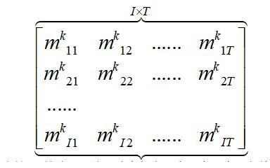
Encode structure and generate initial solution: Each particle is a $I\times T$ matrix, which represents the product production quantity matrix of the T phase. The row of the matrix represents the product varieties and column represents the number of periods. The element in the matrix represents the number of orders assigned to multiple channel k at the T phase of the i product. Each column of the coded structure represents the product variety and the production quantity of each product that the period is to be produced in the multiple channel K. The value of each element of the matrix is an integer that is not less than zero. Using this same encoding structure as the order structure, the tardiness quantity for the particle can be determined directly.
Figure 1. Initial solution of improved PSO
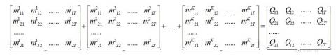
The improved particle swarm algorithm has a strong dependence on the initial solution, and the better initial solution is beneficial to improve the efficiency of the search. For the multistage order varying at any time frame, it is not allowed to delay delivery and can be produced in advance. Therefore, the probability of random initial value, which can not be allowed to delay delivery, can be produced in advance is relatively small. Secondly, the initial value is well constructed, which lays a good foundation for the subsequent steps. Improved the PSO initial value setting based on known resource allocation results (known number of multiple channels, number of workers per multichannel operation, workplace and equipment allocation) and product K matrix of I rows and T columns according to a certain proportion. In the product matrix, each element is a nonnegative integer, and the algebraic sum of K product matrix is equal to the product order matrix. Each multichannel product matrix is a particle.
The choice of the initial value is to produce a multichannel product distribution matrix according to a certain rule under the condition that the number of channels is known, and all the elements of the matrix are integers not less than 0. All multichannel product distribution matrices and matrices are made equal to orders. Whereas the distribution matrix for each multichannel product is a particle.
Step 1: Calculate each multichannel operators in the total proportion of operators $c _ { 1 k } = \frac { r _ { k } } { A } , 0 < c _ { 1 k } < 1$
Step $2 :$ the initial value of the particle group is $c _ { 1 k } * Q _ { i t } .$ where $c _ { 1 k }$ is $\mathrm { k }$ constants obtained in step $1 , Q _ { i t }$ is the input order matrix.
Step 3: k matrices satisfy the following relational formula.
Figure 2. The sum of k matrices
Step 4: The number of operators per channel is known and the beat of each product in each channel can be obtained. According to step 2, the initial value of the improved particle swarm algorithm can be obtained. Replace it with the formula 1 of the scheduling mathematical model, the tardiness number (objective function) of each channel as the initial fitness value of each particle could be obtained.
Improve particle swarm optimization algorithm cross operation: The cross operation in the genetic algorithm and the PSO algorithm are mixed. The cross operation of different particles increases the ability of the particle search space to search for other new positions and avoids the premature falling into the local optimal.
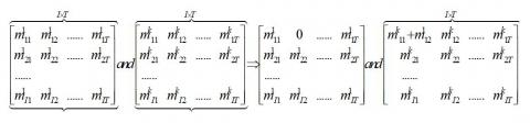
If it is only found in each multiple channel (particle), it is easy to fall into local optimum. In order to broaden the range of optimization, we adjust between multiple particles. For example, by adjusting the $m _ { 12 } ^ { 1 }$ of the first particle to the $m _ { 11 } ^ { k }$ of the $\mathrm { k }$ particle, that is, replace original $m _ { 11 } ^ { k }$ with the $m _ { 12 } ^ { 1 } + m _ { 11 } ^ { k }$ and the original position of $m _ { 12 } ^ { 1 }$ is changed to $0 .$ It can also be locally adjusted. The first step: $A c _ { 2 }$ should be produced first. The second step: Multiply $c _ { 2 }$ by an element that begins with the second column of the first particle, such as $c _ { 2 } \times m _ { 12 } ^ { 1 }$ . The third step: Determine whether the second step results meet the requirements of the minimum batch. Like whether $c _ { 2 } \times m _ { 12 } ^ { 1 }$ and $\left( 1 - c _ { 2 } \right) \times m _ { 12 } ^ { 1 }$ are not less than $B _ { 1 } .$ If it is less than the minimum batch, go back to the first step and revalue. If not less than the minimum batch, replace original $m _ { 11 } ^ { k }$ with the $c _ { 2 } \times m _ { 12 } ^ { 1 } + m _ { 11 } ^ { k }$ and the original position of $m _ { 12 } ^ { 1 }$ is changed to $\left( 1 - c _ { 2 } \right) \times m _ { 12 } ^ { 1 } .$ When $c _ { 2 } = 1 ,$ the cross operation of particle swarm is improved.
Figure 3. Improved cross operation of particle swarm
Improve the variation of individual particle in particle swarm algorithm: Because the delivery cannot be delayed, the initial value adjustment of the particle swarm should start from the second column of the initial value of the particle., and then the elements of the same row in each column may be sequentially or partially adjusted to the same row elements of the column than the column, in turn, in accordance with the bisearch thought.
If it is all adjusted, only a step is required. Like replace original $m _ { 11 } ^ { k }$ with the $m _ { 12 } ^ { k } + m _ { 11 } ^ { k }$ and the original position of $m _ { 12 } ^ { k }$ is changed to $0 .$ If it's a partial adjustment, it takes three steps. The first step: $\mathrm { A } c _ { 1 } = 0.5$ should be produced first. The second step: Multiply $c _ { 1 }$ by an element that begins with the second column, such as $c _ { 1 } \times m _ { 12 } ^ { k }$ . The third step: Determine whether the second step results meet the requirements of the minimum batch. Like whether $c _ { 1 } \times m _ { 12 } ^ { k }$ and $\left( 1 - c _ { 1 } \right) \times m _ { 12 } ^ { k }$ is not less than $B _ { 1 }$ . If it is less than the minimum batch, go back to the first step and revalue. If not less than the minimum batch, replace original $m _ { 11 } ^ { k }$ with the $c _ { 1 } \times m _ { 12 } ^ { k } + m _ { 11 } ^ { k }$ and the original position of $m _ { 12 } ^ { k }$ is changed to $\left( 1 - c _ { 1 } \right) \times m _ { 12 } ^ { k }$.
Figure 4. Improved cross operations of particle swarm
Updated position of particle swarm: Given the speed v, and each feasible solution obtained is its current fit value. Compare the adaptive values corresponding to their individual historical best position (pbest), and update the historical best position pbest with the current position if the current adaptation is higher. Add up the pbest values of all particles as the globally value of the current fitness, and compare with gbest. If the current adaption is better, the position of the current particle is updated to the globally optimal position gbest.
Updated position of particle swarm:
$X_{i}^{k+1}={{c}_{2}}\otimes f\{[{{c}_{1}}\otimes q(w\otimes h(X_{i}^{k}),pB_{i}^{k}),pB_{i}^{k}],g{{B}^{k}}\}$ (17)
Among them, $w , c _ { 1 } , c _ { 2 } \in [ 0,1 ] , p B _ { t } ^ { k }$ is the individual optimal value of k-generation particles, $g B _ { t } ^ { k }$ is the globally optimal value for $K$ generation of particles. $h , q , g , f$ are operators. The formula $( 17 )$ consists of three parts.
The first part is formula $( 18 ) , r \in [ 0 ~ 1 ] .$
$E_{i}^{k}=w\otimes h(X_{i}^{k})=\left\{ \begin{align} & (X_{i}^{k})\begin{matrix} {} & {} & r<w \\\end{matrix} \\ & X_{i}^{k}\begin{matrix} {} & {} & {} & r\ge w \\\end{matrix} \\ \end{align} \right.$ (18)
Look up in the improved mutation operation of particle swarm optimization (PSO).
The second part is the formula (19).
$F_{i}^{k}={{c}_{1}}\otimes q(E_{i}^{k},pB_{i}^{k})=\left\{ \begin{align} & q(E_{i}^{k},pB_{i}^{k})\begin{matrix} {} & {} & {} & r<{{c}_{1}} \\\end{matrix} \\ & E_{i}^{k}\begin{matrix} {} & {} & {} & \begin{matrix} {} & {} & r\ge {{c}_{1}} \\\end{matrix} \\\end{matrix} \\ \end{align} \right.$ (19)
Look up in the cross operations of particle swarm.
$X_{i}^{k}={{c}_{2}}\otimes f(F_{i}^{k},g{{B}^{k}})=\left\{ \begin{align} & f(F_{i}^{k},g{{B}^{k}})\begin{matrix} {} & {} & {} & r<{{c}_{2}} \\\end{matrix} \\ & F_{i}^{k}\begin{matrix} {} & {} & {} & \begin{matrix} {} {} & r\ge {{c}_{2}} \\\end{matrix} \\\end{matrix} \\ \end{align} \right.$ (20)
The formula (20) indicates that the particle swarm is adjusted according to the globally optimal position.
5)Terminal condition When the termination condition of the algorithm is the number of iterations that have been set in advance, the algorithm is terminated.
Step 1: input the number of multiple channels K, the order matrix of the product, the number of iterations G, the inertia constant w and learning factor c1 and c2.
Step 2: Generating a multichannel product distribution matrix according to the proportion of the multichannel operators. All elements of the matrix are integers of not less than 0. Make all multichannel product distribution matrices and matrices equal to the orders. And the distribution matrix of each multichannel product is a particle. The locally optimal solution pBi and the globally optimal solution gBi are calculated.
Step 3: Update the position of the particle according to the mutation operation of the single particle in the improved particle swarm optimization algorithm, and update the locally optimal solution pBi and the globally optimal solution gBi at the same time.
Step 4: The position of particles is further updated according to the cross operation between particles, and the local optimal solution pBi and the global optimal solution gBi are updated at the same time.
Step 5: Judging whether the termination condition (like whether the number of iterations >G) is met, and if so, outputting the optimal solution; otherwise, turning to step 3.
In order to verify the effectiveness of the improved particle swarm optimization algorithm, 13 random examples (i,t,k,h,T) are selected in this section. The order type in the example is a change order at any time. In this paper, the algorithm is compared with the general genetic algorithm, and the experimental optimization algorithm is realized by MATLAB7.0 and PC use Pentium®Dual-Core CPU. The algorithm parameters of this paper are: the number of iterations is 50 times, $w = 0.1 , c _ { 1 } = 0.5 , c _ { 2 } = 0.5$ The results obtained are shown in Table 1. The two scheduling algorithms are run 50 times each, and the optimal solution and the worst solution and the mean solution are obtained in 50 times. The deviations of the two algorithms are obtained from (improved particle swarm optimization algorithm average solution A - genetic algorithm average solution B)/ improve average solution A of particle swarm algorithm. The time deviation is derived from (improved particle swarm optimization algorithm average time T1 - average time T2 of genetic algorithm) / improve average time T1 of particle swarm algorithm. After comparing the two algorithms, we can draw the following conclusions: the improved particle swarm optimization algorithm is superior to the genetic algorithm in terms of the optimal value, the worst value, the average value and the running time of the objective function.
Parameter sensitivity analysis: Further consideration is given to the algorithm deviation of the improved particle swarm optimization algorithm and genetic algorithm for the parameter m, k and t objective functions and the sensitivity of time deviation. As shown in figure 5, when m, k invariant t increases, the algorithm bias and time deviation of the improved particle swarm optimization algorithm are further increased. The same conclusion can also be obtained when t, k is constant, m is increased, or m, t is constant and k increases. And h, T is not sensitive to algorithm deviation and time deviation.
Table 1. Different improved PSO and genetic algorithm
|
example |
improved particle swarm |
genetic algorithm |
deviation of algorithm |
time deviation |
||||||
|
the optimal solution |
the worst solution |
The average solution A |
The average computation time T1 (s) |
The optimal solution |
The worst solution |
The average solution B |
The average computation time T2 (s) |
|
|
|
|
(5,6,2,10,152800) |
484 |
521 |
502.5 |
1.02 |
552 |
538 |
545 |
2.17 |
-8.5 |
-112.7 |
|
(5,6,2,20,152800) |
486 |
524 |
505 |
1.03 |
544 |
558 |
551 |
2.15 |
-9.1 |
-112.7 |
|
(5,6,2,30,152800) |
490 |
527 |
508.5 |
1.05 |
551 |
564 |
557 |
2.16 |
-9.6 |
-112.7 |
|
(5,6,2,60,152800) |
498 |
534 |
516 |
1.02 |
549 |
556 |
552.5 |
2.13 |
-7.7 |
-112.7 |
|
(5,6,4,30,152800) |
454 |
498 |
476 |
1.64 |
535 |
512 |
523.5 |
3.97 |
-9.0 |
-128.1 |
|
(10,6,2,10,172800) |
98 |
125 |
111.5 |
2.56 |
90 |
252 |
171 |
6.24 |
-54.5 |
-143.1 |
|
(10,6,2,60,172800) |
123 |
158 |
140.5 |
2.58 |
136 |
286 |
211 |
6.27 |
-50.1 |
-143.2 |
|
(10,12,2,80,172800) |
138 |
179 |
158.5 |
3.25 |
176 |
319 |
247.5 |
8.29 |
-56.1 |
-155.1 |
|
(10,12,4,100,172800) |
341 |
373 |
357 |
3.96 |
514 |
628 |
571 |
10.21 |
-59.9 |
-157.8 |
|
(10,12,4,120,172800) |
442 |
484 |
463 |
3.98 |
645 |
838 |
741.5 |
10.24 |
-60.06 |
-157.9 |
|
(10,12,8,100,172800) |
378 |
427 |
407.5 |
4.34 |
554 |
757 |
655.5 |
11.45 |
-60.9 |
-168.3 |
|
(16,12,6,100,222800) |
521 |
541 |
531 |
5.85 |
773 |
1078 |
925.5 |
17.13 |
-74.3 |
-192.8 |
|
(16,12,12,100,222800) |
502 |
533 |
517.5 |
6.91 |
836 |
1193 |
1014.5 |
20.96 |
-96.03 |
-203.3 |
|
(16,12,8,100,222800) |
415 |
440 |
427.5 |
6.15 |
671 |
889 |
1999 |
18.43 |
-82.67 |
-199.6 |
|
(16,12,2,100,222800) |
757 |
786 |
771.5 |
5.56 |
1062 |
1308 |
1185 |
13.45 |
-53.8 |
-141.9 |
Figure 5. The sensitivity analysis of the two algorithms for different parameters
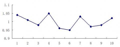
In order to analyze the stability of the improved particle swarm optimization (PSO) algorithm, an order is randomly selected from the generated order for 10 operations. The average of the tardiness is 460.2, and the fluctuation is shown in Fig. 6. In 10 operations, the wave of the objective function is within $\pm 10 \%$. Therefore, it can be seen that the improved particle swarm algorithm has good stability.
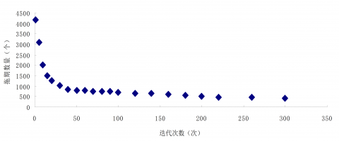
In terms of the convergence of the algorithm, Fig. 7 shows the convergence of the average number of tardiness of the objective function with the number of iterations in the improved particle swarm optimization (PSO) algorithm. The results show that with the increase of the number of iterations, the tardiness quantity tends to decrease. When the number of iterations is more than 300 times, the tardiness quantity tends to a certain stable value. It is proved that the algorithm has good convergence.
Figure 6. The wave of the objective function of algorithm run 10 times
Figure 7. The change of the objective function of algorithm in iterative 300 times
In this paper, we propose a parallel machine scheduling algorithm for the improved particle swarm with multiple variety, multiple period and minimum batch constraints, which takes into account the transition time of the target function as the tardiness quantity. Because the crossover operation is embedded in the particle swarm optimization algorithm, the ability of the particle to search for other new positions in the search space is increased, and the local optimal solution is avoided prematurely. The idea of bisearch increase the search efficiency, so that the speed is fast, and the total tardiness quantity can be well controlled. The main conclusions are as follows:
The algorithm can satisfy the demand of multiple product and multiple period considering the time of delivery, and gives the scheduling scheme with minimum number of tardiness in the parallel production line of robot manipulator, which shows that the algorithm is simple and feasible.
Compared with other scheduling algorithms, the algorithm has many advantages in large scale examples, both in terms of the computation time and the solution of the objective function.
Through the research of this paper, it provides a new solution to the assembly scheduling problem of parallel production line of manipulator considering the changing production time in many varieties and variable batches. The next step will study the assembly calculation and scheduling integrated optimization to improve the manufacturing technology of complex product assembly system execution system.
Anyang city science and technology project.
Aghajani A., Didehbani S. A., Zadahmad M., Seyedrezaei M., Mohsenian O. (2014). A multi-objective mathematical model for cellular manufacturing systems design with probabilistic demand and machine reliability analysis. The International Journal of Advanced Manufacturing Technology, Vol. 75, No. 5-8, pp. 755-770. http://doi.org/10.1007/s00170-014-6084-0
Akbari M., Zandieh M., Dorri B. (2013). Scheduling part-time and mixed-skilled workers to maximize employee satisfaction. International Journal of Advanced Manufacturing Technology, Vol. 64, No. 5-8, pp. 1017-1027. http://doi.org/10.1007/s00170-012-4032-4
Arkat J., Hosseini L., Farahani M. H. (2011). Minimization of exceptional elements and voids in the cell formation problem using a multi-objective genetic algorithm. Expert Systems with Applications an International Journal, Vol. 38, No. 8, pp. 9597-9602. https://doi.org/10.1016/j.eswa.2011.01.161
Azadeh A., Hatefi S. M., Kor H. (2012). Performance improvement of a multi product assembly shop by integrated fuzzy simulation approach. Journal of Intelligent Manufacturing, Vol. 23, No. 5, pp. 1861-1883. https://doi.org/10.1007/s10845-011-0501-0
Book R. V., Karp Richard M. (2014). Reducibility among combinatorial problems. Complexity of computer computations. Proceedings of a Symposium on the Complexity of Computer Computations. Held March 20-22, 1972, at the IBM Thomas J. Watson Center, Yorktown Heights, New York. Journal of Symbolic Logic, Vol. 40, No. 4, pp. 618-619. https://doi.org/10.2307/2271828
Boulif M., Atif K. (2006). A new branch-&-bound-enhanced genetic algorithm for the manufacturing cell formation problem. Computers & Operations Research, Vol. 33, No. 8, pp. 2219-2245. https://doi.org/ 10.1016/j.cor.2005.02.005
Defersha F. M., Chen M. (2008). A linear programming embedded genetic algorithm for an integrated cell formation and lot simulated annealing. European Journal of Operational Research, Vol. 187, No. 1, pp. 46-69. http://doi.org/ 10.1016/j.ejor.2007.02.040
Filho E. V. G., Tiberti A. J. (2006). A group genetic algorithm for the machine cell formation problem. International Journal of Production Economics, Vol. 102, No. 1, pp. 1-21. https://doi.org/10.1016/j.ijpe.2004.12.029
Liu C. G., Li W. J., Lian J., Yin Y. (2012). Reconfiguration of assembly systems: From conveyor assembly line to serus. Journal of Manufacturing Systems, Vol. 31, No. 3, pp. 312–325. https://doi.org/10.1016/j.jmsy.2012.02.003
Liu C. G., Yang N., Li W. J., Lian J., Evans S., Yin Y. (2013). Training and assignment of multi-skilled workers for implementing seru, production systems. International Journal of Advanced Manufacturing Technology, Vol. 69, No. 5-8, pp. 937-959. https://doi.org/10.1007/s00170-013-5027-5
Meller R. D., Deshazo R. L. (2001). Manufacturing system design case study: Multi-channel manufacturing at electrical box & enclosures. Journal of Manufacturing Systems, Vol. 20, No. 6, pp. 445-456. https://doi.org/10.1016/S0278-6125(01)80063-7
Rezazadeh H., Mahini R., Zarei M. (2011). Solving a dynamic virtual cell formation problem by linear programming embedded particle swarm optimization algorithm. Applied Soft Computing, Vol. 11, No. 3, pp. 3160-3169. https://doi.org/10.1016/j.asoc.2010.12.018
Roshani A., Giglio D. (2016). Simulated annealing algorithms for the multi-manned assembly line balancing problem: Minimising cycle time. International Journal of Production Research, Vol. 55, No. 10, pp. 2731-2751. https://doi.org/10.1080/00207543.2016.1181286
Shidpour H., Cunha C. D., Bernard A. (2014). Analyzing single and multiple customer order decoupling point positioning based on customer value: A multi-objective approach. Procedia Cirp, Vol. 17, pp. 669-674. https://doi.org/10.1016/j.procir.2014.01.102
Siemiatkowski M., Przybylski W. (2007). Modelling and simulation analysis of process alternatives in the cellular manufacturing of axially symmetric parts. The International Journal of Advanced Manufacturing Technology, Vol. 32, No. 5, pp. 516-530. https://doi.org/10.1007/s00170-005-0366-5
Song X., Li B. H., Chai X. (2008). Research on key technologies of complex product virtual prototype lifecycle management (CPVPLM). Simulation Modelling Practice & Theory, Vol. 16, No. 4, pp. 387-398. https://doi.org/10.1016/j.simpat.2007.11.008
Yu Y., Gong J., Tang J. F., Yin Y., Kaku I. (2012). How to carry out assembly line–cell conversion? A discussion based on factor analysis of system performance improvements. International Journal of Production Research, Vol. 50, No. 18, pp. 5259-5280. https://doi.org/10.1080/00207543.2012.693642
Yu Y., Tang J., Gong J., Yin Y., Kaku I. (2014). Mathematical analysis and solutions for multi-objective line-cell conversion problem. European Journal of Operational Research, Vol. 236, No. 2, pp. 774-786. https://doi.org/10.1016/j.ejor.2014.01.029
Yu Y., Tang J., Gong J., Yin Y., Kaku I. (2014). Mathematical analysis and solutions for multi-objective line-cell conversion problem. European Journal of Operational Research, Vol. 236, No. 2, pp. 774-786. https://doi.org/10.1016/j.ejor.2014.01.029