OPEN ACCESS
The purpose of this study is to perform a comprehensive analysis on the influence of heavy rain upon the aerodynamic efficiency of two different airfoil structures. A simulation model was performed through the analysis using a commercial software ANSYS. Comparison of the effect of the rainfall was executed by comparing our software simulation output with findings in reported available literature. It is very hard and expensive to evaluate the performance degradation under heavy rain experimentally. This analytical study depicts the consistent degradation of performances of some aerofoil structure under heavy rain. Discrete Phase Modeling (DPM) has achieved considerable accurate result for our simulation for the stall of the aircraft.
angle of attack, lift, drag, DPM, CFD.
During heavy rain, the lift force on airfoil structure is decreased, whereas, the drag is found to be increased. It has been reported that heavy rain up to 1500 mm/h may decrease the lift coefficient up to 20% and increase drag coefficient up to 30% (Haines et Luers, 1983). Heavy rain also affects premature boundary layer in low angle of attack and separation at high angle of attack. In aviation industries, optimized airfoil design capable of tolerating such adverse conditions of heavy rain emerges as a thrust domain of research in order to ensure flight safety and also to enhance its aerodynamic performances. Conventional simulation practice employs three-dimensional CFD models for effective performances of fluid-structure interaction (Emani et al., 2017). Similar trend of aerodynamic performances is also followed in comparative study for aerofoils. Basically rain happens in the low altitude at the time of take-off and landing. Aerodynamic efficiency is basically considered as the ratio of the lift coefficient to drag coefficient, which is degraded by 30-40% at the time of stalling in low altitudes. Here two different aerofoils have been considered for comparative analysis among different parameters under heavy rain situation.
Heavy rain is indicated by the LWC (Liquid Water Content) which is a function of rainfall intensity. For different rain conditions relationship between LWC and rain intensity varies (Joss et Waldvogal, 1969). The previous study of the aerodynamic performance degradation due to rain has been performed by Rhode (1941) who found 18% decrease in performance for the DC-3 aircrafts for LWC 50 g/m3. Haines and Luers (1983) analysed the frequency and intensity of very heavy rains and their effects on a landing aircraft. Hansman and Barsotti (1985) compared the aerodynamic performance degradation of NACA 64-210, NACA 0012, and Wortman FX 67-K170 aerofoils under the low Reynolds numbers in heavy rain conditions. In other similar wind tunnel experiments, laminar flow aerofoils were also found to experience performance degradation approximately equivalent to that caused by tripping the boundary layer to turbulence. On analysis of surface tension interaction of the water of intense rain, Bezos et al., (1992) noticed an aerodynamic degradation. Aerodynamic performance degradation depended on the location and diameter of the rivulet formation and rivulets. Valetine and Decker (1983) also studied the performance parameter of the NACA 64210 aerofoil by tracking the particles. Carlse and Hankey (1984) used two way coupled Euclerian scheme to model rain for NACA 0012 for fine and coarse rain. In fine rain condition, he found that the increase in drag and lift was a function of the fluid density, whereas for the coarse condition they did not find any effective changes.
Two approaches are used to model fluid particle Flow i.e. Euclidian and Langragian model. In Euclidian model, two fluids (basically uniform particle sizes) are taken and both particles and fluid are taken as continuous phase. For each flow, conservation equations are solved by considering the mass, phase exchange, momentum transfer energy transfer. In Langragian model, two approaches are used, one way coupled and two ways coupled. In one way coupled, the particle presence does not affect the trajectories of the continuous phase, but in the two way coupled motions both fluid and particles are interacting with each other. So source terms are added to solve the conservation equations. For the rain model, it is important to establish the size distribution of the water droplets. The wall temperature is responsible for the droplets to be splashed, rebound and stick.
In this present work, wall temperature is assumed to be below than the boiling temperature of the droplet, and only stick, spread and splash are considered here. As the experiment made by Bilanin (1987) described that the evaporation effect does not affect aerodynamic efficiency. So, we have ignored this effect. Therefore, only energy and momentum conservation equations are taken as the conservation equations for the film particles.
Compressible and turbulent air flow and the inert rain particles were considered in this present analysis. Two way coupled Lagrangian equation were used in the solver to analyse the effect of heavy rain on the two cambered NACA 23012 and NACA 2415airfoils, the geometry of which have been modelled using ICEM CFD 14.5. Discrete phase modelling (DPM) in a Lagrangian frame of reference with break up TAB model has been used to simulate the rain particles dispersed in continuous phase using two-phase flow approach with its impact of coupling phase. In DPM, rain particles have been modelled by injected rain particles. Rain particle is assumed to be of spherical shape, non-evaporative, non-spinning and non-reacting with each other. Rain falling angle has been taken as right angle as per the convenience of the calculation. k-€ model has been used for the analysis.
The assumptions are taken here are, the rain particles are non-reacting with each other and non-evaporative as per the past studies by Bilanin (1987). In accordance with the said study, evaporation of the droplets will not influence the aerodynamic performance. Non-deforming and spherical droplets are taken in present study for the simplification of the analysis, but in actual practice the raindrop deforms when they enter inside the boundary layer. For validation purpose XFOIL data was used. XFOIL is an interactive program for the design and analysis of subsonic isolated airfoils. XFOIL provides values of all performance parameters values as an output by taking Reynolds’s number and Mach number as input.
3.1. Scaling of the rain model
Rain is considered as heavy by taking two factors i.e. intensity and frequency of the rain. LWC is chosen for separating different intensity of the rain.
LWC can be written as:
$\left.L W C = \int _ { 0 } ^ { \infty } \rho _ { w } \frac { \pi } { 6 } D ^ { 2 } N ( D ) d D \right)$ (1)
Where, $\rho_w$ is the density of the water
Terminal velocity which is uniform under the action of gravity force and air friction drag force, is found to be a function of mean diameter of the particles and is given by Markowitz (1976) as follows:
$\mathrm { V } ( \mathrm { D } ) = 9.58 \left[ 1 - \operatorname { Exp } \left\{ - \left( \frac { D } { 1.77 } \right) ^ { 1.147 } \right\} \right]$ (2)
Where, D is the mean diameter of the particle. A correction for the aloft is given by Markowitz (1976) as follows:
$\mathrm { V } ( \mathrm { D } ) = \mathrm { V } _ { 0 } ( \mathrm { D } ) \left( \frac { \rho _ { 0 } } { \rho _ { a } } \right) ^ { 0.4 }$ (3)
Where, V0 (D) is the terminal velocity of the particle when density of the air loft is $\rho_0$.
3.1.1. Wall film model
In this model, some assumption has been taken for the easy simulation in software. Basically this model is used to describe the various interactions between rain drops and boundary surface. This interaction includes drop impingement, momentum transfer, droplet evaporation and splashing effect, mass transfer, conduction and convective heat transfer, flow separation etc. The assumption, that have been taken here, are as follows:
1) The water film layer is very thin.
2) The temperature of the film is below the boiling temperature of the water particle.
3) Film particles are assumed to be direct contact with the wall surface so that only conduction heat transfer is possible
The wall temperature is responsible for the droplets to be splashed, rebound, spread and stick. In this case, as the wall temperature is assumed to be below than the boiling temperature of the droplet so only stick, spread and splash are considered here. As the experiment made by Bilanin (1987) described that the evaporation effect does not affect aerodynamic efficiency. Therefore, this effect was ignored this effect. So, only energy and momentum conservation equations were considered in the conservation equations for the film particles. ICEM CFD was used for geometry and hexagonal mesh generation. k-$\in$RNG models was chosen. Forair, ideal gas model has been used which includes both compressibility and Sutherland law as viscosity model. The second order upwind scheme and second order momentum schemes have been used for discrimination to reach at the final result. The governing equations are used here are as follows:
$\frac { \partial \rho } { \partial t } + \frac { \partial \left( \rho u _ { i } \right) } { \partial x _ { i } } = 0$ (4)
$\frac { \partial \rho u _ { i } } { \partial t } + \frac { \partial \left( \rho u _ { i } u _ { j } \right) } { \partial x _ { j } } = - \frac { \partial p } { \partial x _ { i } } + \frac { \partial \left[ \mu \left( \frac { \partial u _ { i } + \partial u _ { j } } { \partial x _ { i } }- \frac { 2 } { 3 }\rho_i \frac { \partial u _ { i } } { \partial x _ { i } } \right) \right] } { \partial x _ { j } } + \frac { \partial ( - \rho \overline { u _ { i } ^ { \prime } u _ { j } ^ { \prime } } ) } { \partial x _ { j } }$ (5)
$- \rho \overline { u _ { \imath } ^ { \prime } u _ { \jmath } ^ { \prime } }$ is Reynolds stress term and k-$\in$turbulent model equations are as follows:
$\frac { \partial ( \rho k ) } { \partial t } + \frac { \partial \left( \rho k u _ { j } \right) } { \partial x _ { j } } = \frac { \partial \left( \alpha _ { k } \mu _ { e f f } \frac { \partial k } { \partial x _ { j } } \right) } { \partial x _ { j } } + G _ { k } + G _ { b } - \rho \in - Y _ { m } + S _ { k }$ (6)
$\frac { \partial ( \rho \in ) } { \partial t } + \frac { \partial \left( \rho \in u _ { j } \right) } { \partial x _ { j } } = \frac { \partial \left( \alpha _ { k } \mu _ { e f f } \frac { \partial k } { \partial x _ { j } } \right) } { \partial x _ { j } } + C _ { 1 \in } \frac { \epsilon } { k } \left( G _ { k } + C _ { 3 \in } G _ { b } \right) - C _ { 2 \in } \rho \frac { \epsilon ^ { 2 } } { k } - R _ { \in } + S _ { k }$ (7)
3.1.2. Two phase modelling
Currently two approaches are being used as Eulerian-Eulerian and Eulerian-Langrangian. In present case, Eulerian-Langrangian approach has been used. This approach treats the fluid as the continuous phase and the particles as the dispersed phase. The particles are tracked, which can exchange as, momentum, energy with the continuous phase. Dispersed phase occupies low volume fraction and high mass flow rate. The track of the dispersed particles can be computed by using the acceleration produced by the force balance equation on the particles, which can be written as follows:
$\frac { d v _ { p } } { d t } = F _ { \text {Drag } } \left( v - v _ { p } \right) + F _ { x }$ (8)
Fx is the additional acceleration term.
FDrag is drag force per unit mass and written as
$F _ { \text {Drag} } = \frac { 18 \mu C _ { d } R e } { 24 \rho p d _ { p } ^ { 2 } }$ (9)
Where, v is the fluid velocity, vp is the particle velocity, $\mu$ is the molecular viscosity of the fluid,
dp is the diameter of the fluid particle, $\rho_p$ is the density of the particle. The relative Reynolds’s number is given by$\operatorname { Re } = \frac { \rho d _ { p } \left| v _ { p } - v \right| } { \mu }$ (10)
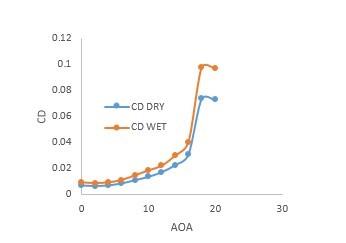
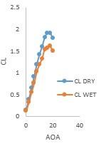
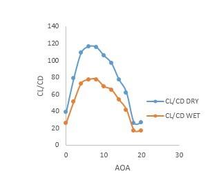
From the, comprehensive comparative results are appended in Table 1, it is observed that in case of NACA 2415 aerofoil drag coefficient (CD) is almost 33% more and lift coefficient (CL) is almost 11% less, therefore, up to about 45%performance has degraded in this case. On the other hand, for the NACA 23012 aerofoil CD has almost 29% more and CL has almost 14% less, which results a drop of performance by about 42%.
Where,
Drag coefficient: CD
Lift coefficient: CL
Angle of attack: AOA
Table 1. Comparative analysis on two aerofoils
|
Aerofoil |
NACA 2415 |
NACA 23012 |
|
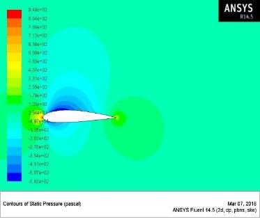
PRESSURE CONTOUR |
||
|
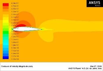
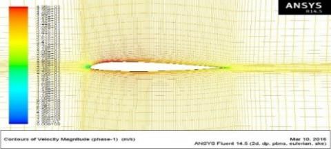
VELOCITY CONTOUR |
||
|
CD Vs. AOA |
||
|
CL Vs. AOA |
||
|
CL/CD Vs. AOA |
4.1. NACA 2415
For this analysis, we have chosen Reynolds’s number for the air flow is nearly about 2.7×10⁶ which is considered to be a turbulent flow. From Reynolds number the free stream velocity of the air has been found to be 40 m/s. The area of the injecting surface is assumed to be 16×1 m2. The distance between two water droplets (scaled length) has been assumed to be 2.15 cm. Thus, 140 injection points were obtained. LWC for heavy rain has been taken here as 25 g/m3. The mean diameter of each droplet has been taken as 0.98 mm. Terminal velocity of each droplet came as 3.813m/s. The mass flow rate of each water particle is calculated and found to be as 2.0426×10⁻³. All this calculation has been done under transient state.
4.2. NACA 23012
For this airfoil Reynolds number for the air flow was taken as nearly about 3×10⁶ which is considered to be a turbulent flow. From Reynolds number the free stream velocity of the air has been found to be 40m/s. The area of the injecting surface is assumed to be 21×1 m2. The distance between two water droplets (scaled length) has been assumed to be 2.35cm. In this way 140 injection points were found. LWC for heavy rain has been taken here as 28 g/m3. The mean diameter of each droplet has been taken as 0.78 mm. Terminal velocity of each droplet has been calculated as 2.48m/s. The mass flow rate of each water particle is calculated and found to be as 1.63294×10⁻³. All this calculation has been done under transient state.
From our software simulation is can be concluded that for the NACA 2415 aerofoil drag coefficient (CD) is almost 33% increased and lift coefficient (CL) is almost 11% reduced, which results a drop of performance by about 45%. On the other hand, for the NACA 23012 aerofoil CD has increased almost 29% and CL has reduced almost 14%, therefore, up to about 42% performance has degraded in this case. This preliminary finding could help for the safety aviation of the flight in stormy and heavy rain climate and the accidents and other severe issues related to heavy rain could be substantially avoided.
Bezos G. M., Jr D. R. E., Jr G, L. G. (1992). Wind tunnel aerodynamic characteristics of a transport-type airfoil in a simulated heavy rain environment. NASA TM-3184. https://ntrs.nasa.gov/archive/nasa/casi.ntrs.nasa.gov/19920022288.pdf
Bilanin A. J. (1987). Scaling laws for testing airfoils under heavy rainfall. Journal of Aircraft, Vol. 24, No. 1, pp. 31-37. https://doi.org/10.2514/3.45407
Carlse W., Hankey W. L. (1984). Numerical analysis of rain. AIAA Report, pp. 84-539. https://doi.org/10.2514/6.1984-539
Emani S., Yusoh N. A., Gounder R. M., Shaari K. Z. K. (2017). Effect of operating conditions on crude oil fouling through CFD simulations. International Journal of Heat and Technology, Vol. 35, No. 4, pp. 1034-1044. Https://doi.org/10.18280/ijht.350440
Haines P. A., Luers J. K. (1983). Aerodynamic penalties of heavy rain on landing aircraft. Journal of Aircraft, Vol. 20, No. 2, pp. 111-119. https://doi.org/10.2514/3.44839
Hansman R. J. J., Barsotti M. F. (1985). The aerodynamic effect of surface wetting effects on a laminar flow air foil in simulated heavy rain. Journal of Aircraft, Vol. 22, No. 12, pp. 1049-1053. https://doi.org/10.2514/3.45248
Joss J., Waldvogal A. (1969). Raindrop size distribution and sampling size error. J. Atmos. Sci., Vol. 26, No. 3, pp. 566-569. https://doi.org/10.1175/1520-0469(1969)026<0566:RSDASS>2.0.CO;2
Luers J. K., Haines P. A. (1983). Heavy rain influence on airplane accidents. Journal of Aircraft, Vol. 20, No. 2, pp. 187-191. https://doi.org/10.2514/3.44850
Markowitz A. M. (1976). Raindrop size distribution expression. Journal of Applied Methodology, Vol. 15, No. 9, pp. 1029-1031. https://journals.ametsoc.org/doi/pdf/10.1175/1520-0450%281976%29015%3C1029%3ARSDE%3E2.0.CO%3B2
Rhode R. V. (1941). Some effects of rain fall on flight of airplanes and on instrument indications. NACA TN903. https://apps.dtic.mil/dtic/tr/fulltext/u2/b814123.pdf
Valentine J. R., Decker R. A., (1983). Tracking of raindrops in flow over an airfoil. Journal of Aircraft, Vol. 32, No. 1, pp. 100-105. https://doi.org/10.2514/3.46689