Moussa Attia* | Fares Zaamouche | Ala Houam | Rabah Daouadi
© 2022 IIETA. This article is published by IIETA and is licensed under the CC BY 4.0 license (http://creativecommons.org/licenses/by/4.0/).
OPEN ACCESS
This study of modifying the frame forces of an electric vehicle offers benefits for controlling stability. We used a two-wheeled self-driving electric vehicle in this study. Taking into account important parameters such as vehicle speed, the vehicle's stability criterion is determined based on the torque level and lateral slip angle. It is equipped with a traction control system that integrates its dynamic system with a sporty design. This level of control improves the vehicle's stability and safety. A conventional regulator has been developed and trained to apply motor control to a sophisticated power supply system. The stability of the EVs was controlled by a simulation model. We validated the proposed stability criterion, and the wheel torque control algorithm. Stability control for two-wheeled autonomous vehicles can be developed on the basis of related research. We would like to stress that the controller can be used in a variety of modern electric vehicles because it is so easy to use. An overview of the modeling and simulation results for this system in the MATLAB-Simulink environment will be presented.
electric vehicles, internal combustion vehicles, battery, wheel, modeling, simulation
One of the most popular research topics nowadays is the need for green vehicles that emit exhaust waste with as few hazardous chemicals as possible. These vehicles also consume less fuel. This is the result of technological advances and the desire to protect the environment [1].
Both plug-in hybrid electric vehicles and battery electric vehicles are frequently referred to as "green" because they significantly reduce greenhouse gas emissions. However, the number of electric cars that can be sold to consumers concerned about driving and the number of greenhouse gases that electric power plants that charge electric vehicle batteries emit will determine the real reductions in greenhouse gases. At best, 25% of greenhouse gas emissions could be reduced, and less than 67% could be excluded from oil use. However, if all current vehicles were swapped for fuel cell electric vehicles that run on hydrogen from natural gas, greenhouse gas emissions would be cut by 44% and oil use by more than 100% [1].
Alternatives to internal combustion vehicles (ICVs) are being sought due to how traffic development and related environmental issues are affecting people's quality of life. One of the more exotic options is an electric vehicle (EV) [2].
With research and development of electric vehicles on the road, major auto manufacturers now have to build battery electric vehicles that are feasible and function appropriately; The main limitation relates to the storage capacity of the battery. Alternative variants using hybrid and fuel cell technology are in progress or have already been introduced to the market [3].
Battery-powered road vehicles have other benefits besides those that reduce their negative impact on the environment. By taking advantage of the superior and more precise aerodynamic performance of electric motors, which allows them to manage the torque generated more effectively than internal combustion engines, they can become more attractive [4].
The primary power of this electric motor can be used to regulate the traction force that shows the position between the wheel and the ground. When compared to conventional vehicles, the improved vehicle stability and safety enable higher performance in restricted environments [5].
Traction control and/or anti-lock (ABS or anti-slip) systems are features of some of today's more expensive ICVs. When the accelerator pedal is depressed too hard, traction control devices are used to stop the drive wheels from turning [6].
Anti-lock systems are also available to prevent the wheels from slipping when the brakes are applied. When it detects a tendency to lock up, this technique lowers the braking force, extending the range of slip levels required for the best vehicle performance. With the help of these devices, the vehicle's steering capabilities, stability, and stopping distances should be improved. They're expensive, take up a lot of space, and sometimes don't work up to par [7].
This system is intended to be more user-friendly and compatible with electric vehicles. The implementation of traction wheel drives under separate control (two or four) and the inherent ability of electric motors to control the output torque can provide high traction control with cheap cost, fast reaction, and simple design implementation. By minimizing the energy lost when skidding via friction between the wheel and the road conditions, effective traction control will reduce energy consumption. This will increase the life of the tires [8].
Adding a vehicle body to the proposed design simplifies the mechanical construction of the vehicle. It is possible to use an electric differential instead of a mechanical differential when using two independent two-wheel drives [2].
The vehicle can now steer and stabilize as the torque of each wheel can now be controlled. The traction control algorithm that will be used will be responsible for this [9].
Below, we'll outline a prototype entire system simulation and offer traction control system recommendations. This results in the accurate and rapid movement of both drive wheels in a straight line to the right, and the car's slip-free course on a curved track is made possible by the difference in speed. The study offered both PI control and system analysis. Additionally, a thorough traction control algorithm is described, along with simulations that show how successful it is. We would like to draw attention to the fact that the suggested algorithm may be used for various makes and models of both new and used passenger cars because it is inexpensive and simple to use [5, 9].
The initial goal is to reduce the mechanical transmission components of the system and research various propulsion topologies. The additional benefits of adopting electric propulsion systems correspond to the ability to imagine alternate configurations to the conventional approach. This approach consists of one central motor and many mechanical transmission systems [10].
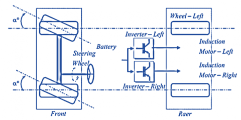
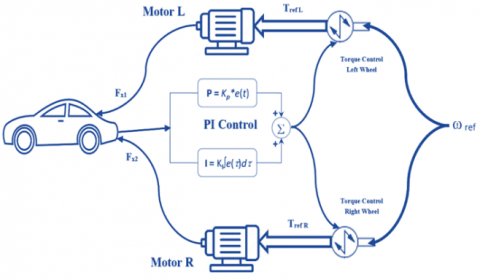
To build an electric vehicle using two distinct front-wheel systems, a diverse variety of topologies were tested. A traction control system is integrated with two asynchronous motors for two independent wheels, as shown in Figure 1.
Figure 1. Electric vehicle propulsion system with two independent wheel drives
The implemented system (composed of electrical and mechanical parts) is shown in Figure 1 within the Matlab-Simulink® environment.
The following succinct statement encapsulates the suggested control system principle: Each motor's torque is regulated by a sliding mode control current loop, and each front wheel's speed is managed by speed difference feedback.
The system was initially modeled using a generalized model. A detailed description of the operation and characteristics of batteries, static converters, wheels, and transmission systems is provided in this model. A force that opposes another is also described [11].
3.1 Speed of the vehicle
The vehicle's speed (vV) can be regarded as being equal to those speeds if the left side (vL) and right side (vR) speeds are equal. The left and right side speeds, though, differ whenever the vehicle describes a circle ($v_L \neq v_R$). Eq. (1) [11] can be used to determine that the vehicle speed is the average of the two speeds.
$v_v=\frac{V L+V R}{2}$ (1)
The vehicle's mass (M) and overall resistance power must be equal to the right and left sides to calculate the speed of the left and right vehicles. Based on Eq. (2), Eq. (3) [11] represents the right side of the vehicle, where AR is the opposing acceleration.
$\vec{F}_R-\frac{\vec{F}_t}{2}=\frac{M}{2} \vec{a}_R \Rightarrow \vec{a}_R=\frac{2}{M}\left(\vec{F}_R-\frac{\vec{F}_t}{2}\right)$ (2)
$\vec{v}_R=\int_0^t \vec{a}_R d t$ (3)
Likewise on the left side [12]:
$\vec{F}_L-\frac{\vec{F}_t}{2}=\frac{M}{2} \vec{a}_L \Rightarrow \vec{a}_L=\frac{2}{M}\left(\vec{F}_L-\frac{\vec{F}_t}{2}\right)$ (4)
$\vec{v}_L=\int_0^t \vec{a}_R d t$ (5)
3.2 Drive dynamics for wheels
Each wheel drive can be described mechanically by the Eq. (6) [12].
$J_m \frac{d \omega_m}{d t}=C_m-C_r$ (6)
In this calculation, Cm, is the motor torque generated, and m is the rotational vehicle speed. Given that a reduction gear is being used and has a transmission ratio of m, the motor reference's loaded torque may be calculated using the formula (7), where R is the tire radius and FRT is the resistance force [12].
$C_r=R \frac{F_{R T}}{\mathrm{~m}}$ (7)
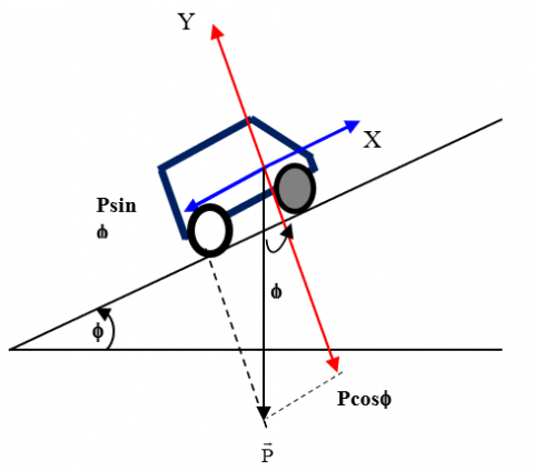
The full moment of the vehicle's acceleration is given by the Eq. (8), which was extracted from the forces shown in Figure 2, as determined by the motor basis (Jm), is the product of the shaft inertial moment, which comprises the motor and wheels inertia (Jwheel), and the component proportional relating to vehicle weight (JV).
$J_m=J_{w \text { heel }}+J_v$ (8)
In Eq. (9), we will define shaft inertia moment JV, where λ is the slip.
Figure 2. Consented to the climbing force's activity
$J_v=\frac{1}{2} M \frac{R^2}{m^2}(1-\lambda)$ (9)
3.3 Total load force, Ft
Four forces contribute to this force: rolling resistance, Stokes force, aerodynamic drag, and climbing resistance [13].
$F_{R t}=F_{r e}+F_{s t}+F_{a d}+F_{c l}$ (10)
The rolling resistance, Fre, in Eq. (10), is calculated using the formula (11) where M is the vehicle's mass, and g is the gravitational acceleration constant. The trying-to-roll resistance, fr, is created by the contact between the road and the tire [13].
Formula (11) is used to determine the friction force, or Fre, in Eq. (10), where M is the vehicle's mass and g is the gravity constant. The tire's contact with the road produces rolling resistance or fr [13].
$F_{r e}=\mathrm{f}_{\mathrm{r}} \cdot M \cdot g$ (11)
When v is the vehicle's speed and kA is the Stokes coefficient, the result is the Stokes force, often known as viscous friction, or Fst [13].
$F_{s t}=K_s v$ (12)
The air resistance to the movement of the vehicle is called aerodynamic drag, and it is calculated by (13) in this way [13].
$F_{a d}=\frac{1}{2} \cdot \rho \cdot A \cdot C_x \cdot\left(v \pm v_v\right)^2$ (13)
When Fcl is positive or negative, respectively, the resistance to the ascent or declimbing is determined by (14) [13].
$F_{c l}=M g \sin \varphi$ (14)
3.4 Equations for longitudinal and lateral vehicle motion
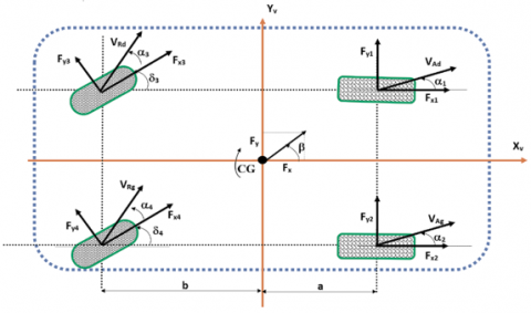
To investigate the dynamics of vertical and horizontal vehicle motion, a variety of statements and models can be applied. The model shown in Figure 3 is one of these. It makes use of a coordinate system based on the chassis.
Vehicle characteristics are shown in Table 1.
Table 1. The different variables of electric vehicles
|
Variables |
Significance |
|
Fyi |
Forces acting on the tire i |
|
Fxi |
Tire transversal forces i |
|
a |
Front axle's separation from CG |
|
b |
CG position from the rear axle |
|
2d |
Wheel spacing on the right and left sides |
|
β |
The angle of the chassis slide |
|
δ |
The freewheel rotation angle |
|
Vx |
Longitudinal speed |
|
Vy |
Lateral speed |
|
V |
Vehicle speed |
|
M |
The vehicle's overall weight |
|
CG |
Point of gravity |
|
θ |
Angle of vehicle rotation |
|
$\alpha \mathrm{i}$ |
Angle of wheel slip |
Newton's second law's differential equations of motion, when applied to the aforementioned vehicle, are as follows:
$\left\{\begin{array}{l}F_x=M \gamma_x \\ F_y=M \gamma_y \\ M=I_z \theta\end{array}\right.$ (15)
Figure 3. The vehicle model's coordinates and variables
Iz stands for the moment of inertia associated with the Z-axis gy for accelerates laterally, and m for the mass of the vehicle. The resultant pitch angle moment that the wheels concerning the vehicle is M, where FX, Fy are the horizontal and vertical forces, consecutively [14]. The effects of the force exerted by the X-axis on the vehicle, comprising the mechanical drag force and the weight element caused by the gradient of the road, are as follows [11]:
$M\left[{V_y}+V_x({\theta}+{\beta})\right]=F_{x 1}+F_{x 2}+\left(F_{y 3}+F_{y 4}\right) \cos \delta_R-\left(R_{r 3}+R_{r 4}\right) \cos \delta_R-\frac{1}{2} \rho C_x A v^2-M g \sin \phi$ (16)
Comparably, the forces moving in the direction of Y are as follows [11]:
$M\left[{V}_y+V_x({\theta}+{\beta})\right]=F_{y_1}+F_{y 2}+\left(F_{y_3}+F_{y 4}\right) \cos \delta_R-\left(R_{r 3}+R_{r 4}\right) \sin \delta_R$ (17)
The full moment of rotational inertia about the center of gravity is [11]:
$\begin{aligned} I_z {\theta}= & {\left[\left(F_{x 1}-F_{x 2}\right)+\left(R_{r 3}-R_{r 4}\right) \cos \delta_R\right.} \left.-\left(F_{y 3}+F_{y 4}\right) \sin\delta_R\right] d-\left(F_{y 1}+F_{y 2}\right) a-b\left(F_{y 3}+F_{y 4}\right) \cos \delta_R-b\left(R_{r 3}+R_{r 4}\right) \sin \delta_R\end{aligned}$ (18)
3.5 The "magic formula" of tires
The powerful tires and points where the vehicle and road come into contact are described by the tire model [12]. Models for pneumatic tires were developed through extensive research and testing. For non-linear tires, the "magic formula tire model" is employed [5].
Calculations are made to determine the tire's lateral and longitudinal forces using [12]:
$F_x=D_x \sin \left(C_x \tan ^{-1}\left(B_x \phi_x\right)\right)+S_{v x}$ (19)
$F_y=D_y \sin \left(C_y \tan ^{-1}\left(B_y \phi_y\right)\right)+S_{v y}$ (20)
where:
$\phi_x=\left(1-E_x\right)\left(\lambda+S_{h x}\right)+\frac{E_x}{B_x} \tan ^{-1}\left(B_x\left(\alpha+S_{h x}\right)\right)$ (21)
$\phi_y=\left(1-E_y\right)\left(\lambda+S_{h y}\right)+\frac{E_y}{B_y} \tan ^{-1}\left(B_y\left(\alpha+S_{h y}\right)\right)$ (22)
Bx, Cx, Dx, Ex, By, Cy, Dy, Ey, Svx, and Svy are constants based on the wheel force given in Eqns. (19, 20, 21, and 22).
We can design a traction control algorithm owing to the capabilities of in comparison to internal combustion motors, electric vehicles display a better flow behavior for managing the created torque [13].
Knowing the actual vehicle speed as well as the velocity of every drive wheel (vW) is important for implementing traction control (vv). It is possible to determine the slip ($\lambda$) (specifically, the relative velocity disparities as described by the equation) using those speeds (23) [5].
$\lambda=\left|\frac{v_{\mathrm{W}}-v_{\mathrm{v}}}{\max \left(v_{\mathrm{W}}, v_{\mathrm{V}}\right)}\right|$ (23)
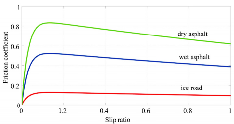
The condition of the road and the amount of produced motor torque both impact the slip value. Eq. (24), which describes the traction or friction coefficient, is shown in Figure 4. In the equation, the force that each wheel and tire may transmit horizontally on the roads is denoted by the symbol Fd (24) [5].
$\mu=\frac{\mathrm{F}_{\mathrm{d}}}{\mathrm{Mg}}$ (24)
Figure 4. According to the slip, the friction coefficient
Controlling all-wheel drive is the responsibility of EV management controllers.
It is crucial to confirm that, when the slip is high, each wheel driver will "see" the vehicle's mass as having a smaller value, as described by Eq. (9). Here, boosting the motor's output torque might be damaging, increasing slip and reducing the traction force being applied to the road [14].
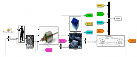
The vehicle model utilized in the investigation and development of the suggested traction control algorithm is shown in Figure 5.
Figure 5. System control structures
The acceleration pedal angle influences the command torque TRef. Feedback from the relative speed differential between the two front wheels is used to manage each front wheel's speed ( $\mathrm{V}_{w \mathrm{R}}, \mathrm{V}_{w \mathrm{~L}}$) [15]. To achieve zero static error between the measured difference value $\Delta \omega=R / 2 d\left(V_{w R}-V_{w L}\right)$ and the reference value for the relative speed difference ($\Delta \omega_{\text {ref }}$), a PI controller is designed. When a discrepancy is found, the controller should adjust the torque reference to each motor using the torque trot (Tref R and Tref L).
Figure 6. Simulink model of an EV wheel drive system proposed
Using Matlab/Simulink, we verify the torque and speed conditions of EVs in Figure 1, which shows the prototype's front-wheel drive and rear-wheel drive systems independently controlled.
In the front-drive system, in order to efficiently generate torque and improve steering ability in congested traffic, a low-speed permanent-magnet synchronous motor (PMSM) is used.
By coupling a differential gear to the motor rotor, to the appropriate wheels, driving torque is transferred.
Moreover, individual controllers and PWM inverters are used to control the wheel drive systems.
As a result, the front wheel distributed torque rendering is optimized based on operating conditions and results in an improved EV's efficiency at higher speeds.
Examining the EV-wheel-drive system is performed in order to describe its characteristics, such as its behavior, speed, and torque simulations are performed using the Matlab/Simulink model that is depicted in Figure 6.
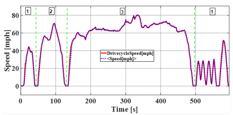
The following Figure 7 shows the speed of the vehicle. It can be subdivided into three intervals or into three micro-paths:
Group 1 micro-paths have a low speed. It lasts for about 40 seconds. The Group 1 micro-paths typically represent the beginning or finish of a journey and necessitate a significant amount of local driving.
While group 2 micro-paths likewise move slowly, they do so more quickly than group 1 does. Additionally, it lasts longer than it did in group 1. Under various driving circumstances, this micro-path is primarily driven by collectors.
The longest duration, biggest deceleration, and highest average speed are all characteristics of Group 3 micro-paths, which also have little time for idling. The micro-path simulates travel on busy roads, including freeways.
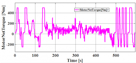
The following Figure 8 shows the shape of the motor torque for different phases, such as acceleration, deceleration and braking mode.
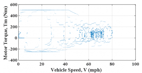
The following Figure 9 represents the mechanical characteristic of the torque as a function of the speed of the vehicle.
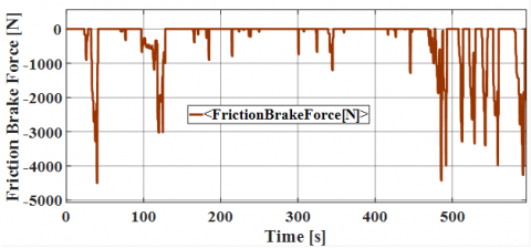
The friction force due to braking is represented by the following Figure 10. We note that, regenerative braking is specific to electric vehicles and makes it possible to transform the vehicle's kinetic energy into electrical energy during a deceleration phase. The converted electrical energy is stored in the battery.
Figure 7. The speed of the vehicle
Figure 8. The speed of the vehicle
Figure 9. The mechanical characteristic of the motor vehicle
Figure 10. The friction brake force
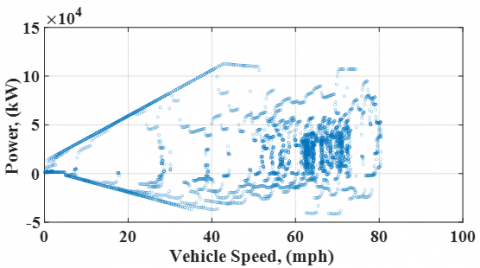
The Figure 11 shows the electromechanical characteristic of the power battery as a function of the speed of the vehicle.
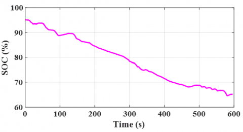
Battery SOC is shown in Figure 12. Since the initial SOC is anticipated to be 95%, the vehicle controller activates the battery to supply the necessary propulsion power.
Figure 11. The electromechanical characteristic between the battery power and the vehicle speed
Figure 12. The battery SOC
This paper describes a two-wheeled electric vehicle. A full system simulation model is described below, along with suggestions for traction control systems.
The use of an electric differential ensures that both drive wheels move precisely and quickly in a straight line to the right and that the difference in speeds provides a slip-free trajectory for the vehicle on a curved track. Both system analysis and PI control were presented in the study.
Also presented is a comprehensive algorithm for controlling traction, as well as simulations illustrating its effectiveness.
We would want to highlight the fact that the suggested algorithm can be implemented on different types of used and newly produced passenger vehicles, as it is low-cost and easy to implement.
The main limitation remains the capacities of the batteries which affect the profitability of electric vehicles compared to traditional technologies.
The association also points to the problem of electricity supply: a complete replacement of the fleet by electric vehicles would lead to an increase in needs of 15%.
This also entails expanding investment in renewable energies. In the future works, real-time implementation of this algorithm control in a MicroAutobox/dSPACE card will be conducted.
[1] Cunanan, C., Tran, M.K., Lee, Y., Kwok, S., Leung, V., Fowler, M. (2021). A review of heavy-duty vehicle powertrain technologies: Diesel engine vehicles, battery electric vehicles, and hydrogen fuel cell electric vehicles. Clean Technologies, 3(2): 474-489. https://doi.org/10.3390/cleantechnol3020028
[2] Larminie, J., Lowry, J. (2012). Electric vehicle technology explained. John Wiley & Sons. https://doi.org/10.1002/9781118361146
[3] Sorlei, I.S., Bizon, N., Thounthong, P., Varlam, M., Vehiclecadea, E., Culcer, M., Raceanu, M. (2021). Fuel cell electric vehicles—a brief review of current topologies and energy management strategies. Energies, 14(1): 252. https://doi.org/10.3390/en14010252
[4] Baroutaji, A., Wilberforce, T., Ramadan, M., Olabi, A.G. (2019). Comprehensive investigation on hydrogen and fuel cell technology in the aviation and aerospace sectors. Renewable and sustainable energy reviews, 106: 31-40. https://doi.org/10.1016/j.rser.2019.02.022
[5] Foito, D., Esteves, J., Maia, J. (2001). Dynamic analysis of a two independent wheel drives electric vehicle, with a traction and a stability control system. In 2001 European Control Conference (ECC), pp. 271-276. https://doi.org/10.23919/ECC.2001.7075918
[6] Heißing, B., Ersoy, M. (2011). Chassis Control Systems. In Chassis Handbook, pp. 493-556. https://doi.org/10.1007/978-3-8348-9789-3_7
[7] Aksjonov, A., Vodovozov, V., Augsburg, K., Petlenkov, E. (2018). Design of regenerative anti-lock braking system controller for 4 in-wheel-motor drive electric vehicle with road surface estimation. International Journal of Automotive Technology, 19(4): 27-742. https://doi.org/10.1007/s12239-018-0070-8
[8] Mohan, H., Pathak, M.K., Dwivedi, S.K. (2020). Sensorless control of electric drives–a technological review. IETE Technical Review, 37(5): 504-528. https://doi.org/10.1080/02564602.2019.1662738
[9] Wei, H., Zhang, N., Liang, J., Ai, Q., Zhao, W., Huang, T., Zhang, Y. (2022). Deep reinforcement learning based direct torque control strategy for distributed drive electric vehicles considering active safety and energy saving performance. Energy, 238: 121725. https://doi.org/10.1016/j.energy.2021.121725
[10] Inal, O.B., Charpentier, J.F., Deniz, C. (2022). Hybrid power and propulsion systems for ships: Current status and future challenges. Renewable and Sustainable Energy Reviews, 156: 111965. https://doi.org/10.1016/j.rser.2021.111965
[11] Lekshmi, S., PS, L.P. (2019). Mathematical modeling of Electric vehicles-A survey. Control Engineering Practice, 92: 104138. https://doi.org/10.1016/j.conengprac.2019.104138
[12] Wang, J., Wang, Q.N., Wang, P.Y., Zeng, X.H. (2014). The development and verification of a novel ECMS of hybrid electric bus. Mathematical Problems in Engineering, 2014. http://doi.org/10.1155/2014/981845
[13] Bouteldja, M., El Hadri, A., Cadiou, J.C., Dolcemascolo, V. (2007). Application of a non-linear sliding mode observer for truck tyre forces estimation. International Journal of Vehicle Systems Modeling and Testing, 2(1): 16-37. http://dx.doi.org/10.1504/IJVSMT.2007.011424
[14] Kahraman, K., Senturk, M., Emirler, M.T., Uygan, I.M. C., Aksun-Guvenc, B., Guvenc, L., Efendioglu, B. (2020). Yaw Stability Control System Development and Implementation for a Fully Electric Vehicle. arXiv preprint arXiv: 2012: 04719. http://doi.org/10.48550/arXiv.2012.04719
[15] De Pinto, S., Chatzikomis, C., Sorniotti, A., Mantriota, G. (2017). Comparison of traction controllers for electric vehicles with on-board drivetrains. IEEE Transactions on Vehicular Technology, 66(8): 6715-6727. https://doi.org/10.1109/TVT.2017.2664663