Yassa Nacera | Houassine Hamza | Ouadfel Ghania* | Rachek Mhemed
© 2022 IIETA. This article is published by IIETA and is licensed under the CC BY 4.0 license (http://creativecommons.org/licenses/by/4.0/).
OPEN ACCESS
This paper presents a new method for modeling the steady-state behavior of the currents transmitted between the windings of a transformer subjected to an inter-turn short-circuit fault (ITSC). ITSC is one of the most frequent and most damaging faults in magnetically coupled circuits, which occur in power transformers. Coupled Electromagnetic Circuit (CEMC) Model modeling the reasoning and relationships describing the operating principle of a power transformer through the electrical and magnetic parameters defined by the self and mutual inductances that influence the voltages and currents transmitted between the transformer windings. The representation of the state variable equations of a proposed model of a three-phase multi-turn transformer in healthy mode (no fault) and in degraded mode (with inter-turn short-circuit faults of 10%, 20% and 30%) has been implemented using a program inserted in MATLAB software. The simulations illustrate the evaluation of the primary and secondary currents as well as the voltage drop across a load, and the accuracy of the state model based on the coupled circuits was validated. The results obtained can provide a basis for the design of the short circuit of the multi-turn transformer.
inter-turn fault, multi-turn transformer, state model, coupled circuits
Currently, the electricity demand is increasing and the investment in power generation and distribution infrastructure is growing [1]. Power transformers are one of the most important components of power systems. Each transformer is designed to withstand several stresses (mechanical, dielectric, thermal), both nominal and due to disturbances (lightning, short circuit, etc.) [2, 3] of different sizes, which partly reflect the operating conditions, an accidental change affecting the normal operation. Therefore, assessing the condition of transformers during their operating life is crucial to ensure their continuity of service and the reliability of the power system [4]. Different types of faults can occur in transformers with varying degrees of severity depending on the extent of the damage caused and its impact [5]. Some faults develop slowly and do not present an immediate danger to the equipment (vibrations, partial discharges) [6]. It is possible, with a little warning, to postpone the repair of the equipment to an appropriate time. Incidents that can cause significant damage and require immediate and automatic intervention are short circuits and internal ignitions.
This work focuses on the study of the effect of inter-winding shorts, which is characterized by abnormal electrical contact between windings of the same coil that should normally be isolated from each other [7]. This often occurs as a result of prolonged dielectric breakdown between windings, or tearing of the insulation paper as a result of severe mechanical deformation of the windings [8]. This fault can lead to the melting of the copper conductors and in some cases to the opening of the electrical circuit. Short circuits between windings can occur at different locations in the windings. When a short circuit fault occurs, a current, called a circulating current due to the occurrence of a low impedance, flows through the shorted windings [9]. This current will also generate an electromagnetic field that will disturb the field transmitted to the secondary [10]. Generally, the effect of a short circuit is to disturb the magnetic flux distribution [11]. On the other hand, the current flowing in the short-circuited turns can reach high values, but the terminal currents do not change much, the homo-polar flux of the magnetic field will dissipate by thermal effect, The result is a rapid destruction of the insulating material covering the core and the conductors belonging to these short-circuited turns, which will spread to the other turns of the transformer winding. Therefore, the need to develop a general model to detect and identify the fault is an obvious step. Different modeling formulations have been developed in the literature to solve these equations. Numerical models (finite element models) give a good accuracy and all physical phenomena are considered [12]. But their disadvantage is the computation time. This remains acceptable in the two-dimensional case, but becomes very important in the three-dimensional case. The permeance network modeling presents a good compromise between calculation time and accuracy. It is based on the decomposition of the structure to a set of reluctances modeling the flow passages. The disadvantage of this method is the assumption of a priori knowledge of the flow knowledge of the flux lines, which forces the designer to take into account all the possibilities [13, 14]. The coupled magnetic circuit model is more complete and closer to physical reality since the number of electrical circuits considered can correspond to all circuits physically installed in the transformer. Among these formulations, we will present those that are best suited to the modeling of transformers. The study of inter-turns short-circuit faults is studied by analyzing the magnetically coupled electrical circuit [15], whose main characteristic is linear inductance. The equations of the circuit are formulated in state variables and simulations illustrate the evolution of the current and voltage for different sets of parameters under load and at no load. The main motivation for studying this fault from a circuit theory point of view is to understand and estimate the consequences of the occurrence of this fault in power transformers.
2.1 Model of a power transformer
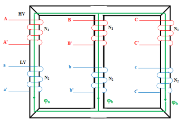
The device is a three-phase column transformer shown in Figure 1, and the method of magnetically coupled circuits is used for the mathematical equation of the windings. This method consists of expressing the self and mutual inductive effects between multiple turns. As we have here coils of simple geometry, these inductances are calculated by analytical expressions. The analytical solution of such equations usually requires simplifying hypotheses.
Figure 1. Three-phase column power transformer
2.2 Simplifying hypothesis
For the mathematical modeling of a power transformer, hypotheses have been made:
- The geometry studied is rotationally asymmetric, the windings are concentric.
- The iron losses are neglected.
- The saturation of the magnetic circuit is neglected.
- The magnetic circuit is linear.
- Constant self and mutual inductance, the leakage inductance is neglected.
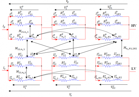
The modeling of transformers consists in establishing a mathematical structure that describes all the electromagnetic phenomena. Skin and proximity effects are the consequences of fields induced in a coil by itself or by neighboring coils. These effects can be expressed as self and mutual inductances through the coupled circuit method. In the absence of a magnetic circuit, the equivalent electrical diagram is a series-parallel associative network of resistors R and self-inductances L and mutual inductances M. A complete equivalent diagram describes the operation of the transformer, as shown in Figure 2.
The transformer is powered by a sinusoidal voltage Vp, delivering a voltage Vs and has currents Ip in the primary and Is in the secondary through it. The transformer is basically characterized by the following system of equations.
Figure 2. Equivalent electrical diagram of HV and LV windings of a power transformer
2.3 Electrical equations
The law of meshes applied to the equivalent electrical diagram of a transformer gives the Eqns. (1)-(11):
$\left[V_{P}\right]=\left[R_{P}\right]\left[I_{P}\right]+\frac{d}{d t}\left[\phi_{P}\right]$ (1)
$\left[V_{S}\right]=\left[R_{S}\right]\left[I_{S}\right]+\frac{d}{d t}\left[\phi_{S}\right]$ (2)
$N_{P}\left[I_{P}\right]=N_{S}\left[I_{S}\right]=\mathfrak{R} \phi$ (3)
$\mathfrak{R}=\frac{\mu S}{l}$ (4)
[Vp] The primary voltage vector.
$\left[V_{s}\right]$ The vector of secondary voltages.
[Ip] The current through the primary winding.
[Is] The current through the primary winding.
$\left[V_{P}\right]=\left[\begin{array}{llll}V_{1}^{p} V_{2}^{p} V_{3}^{p} & \ldots & \ldots\end{array} . V_{N 1}^{p}\right]$ (5)
$\left[I_{P}\right]=\left[\begin{array}{llll}I_{1}^{p} I_{2}^{p} I_{3}^{p} & \ldots \ldots \ldots . \ldots I_{N 1}^{p}\end{array}\right]$ (6)
$\left[I_{1}^{p}\right]=\left[I_{11} I_{21} I_{31} \ldots \ldots \ldots \ldots I_{n_{1} 1}\right]$ (7)
$\left[I_{2}^{p}\right]=\left[I_{12} I_{22} I_{32} \ldots \ldots \ldots \ldots . I_{n_{1} 2}\right]$ (8)
$\left[\begin{array}{c}I_{N 1}^{p}\end{array}\right]=\left[\begin{array}{llll}I_{1 N 1} I_{2 N 1} I_{3 N 1} & \ldots \ldots \ldots . . I_{n_{1} N 1}\end{array}\right]$ (9)
$\left[I_{1}^{p}\right],\left[I_{2}^{p}\right], \ldots\left[I_{N 1}^{p}\right]$ the currents through the primary elementary spires. In windings, magnetic phenomena can be summarized by an inductance coefficient linking the flux to the current that gives rise to it.
$\left[\phi_{P}\right]=\left[L_{P P}\right]\left[I_{P}\right]+\left[M_{p s}\right]\left[I_{s}\right]$ (10)
$\left[\phi_{P}\right]=\left[L_{s s}\right]\left[I_{s}\right]+\left[M_{s p}\right]\left[I_{P}\right]$ (11)
With [Rp], [Lpp], [Rs], [Lss] are the matrices of resistances and inductances of the primary and secondary respectively.
$\left[R_{P}\right]=\left[\begin{array}{cccccc}R_{11} & 0 & \cdots & 0 & \cdots & 0 \\ 0 & \ddots & \vdots & \vdots & \vdots & \vdots \\ 0 & 0 & R_{n} & \vdots & \vdots & \vdots \\ \vdots & \vdots & 0 & R_{12} & \vdots & \vdots \\ \vdots & \vdots & \vdots & 0 & \ddots & \vdots \\ 0 & \cdots & \cdots & \cdots & \cdots & R_{n_{1} N 1}\end{array}\right]$ (12)
$\left[M_{s p}\right]=\left[\begin{array}{ccccccc}M_{11}^{S} & M_{21}^{S} & \cdots & M_{n_{2} 1}^{S} & M_{12}^{S} & \cdots & M_{n_{2} N 2}^{S} \\ M_{11}^{S} & \vdots & \vdots & \vdots & \vdots & \vdots & \vdots \\ \vdots & \vdots & \vdots & \vdots & \vdots & \vdots & \vdots \\ \vdots & \vdots & \vdots & \vdots & \vdots & \vdots & \vdots \\ \vdots & \vdots & \vdots & \vdots & \vdots & \vdots & \vdots \\ \vdots & \vdots & \vdots & \vdots & \vdots & \vdots & \vdots \\ M_{11}^{S} & \cdots & \cdots & \cdots & \cdots & \cdots & M_{n_{2} N 2}^{S}\end{array}\right]$ (13)
$\left[L_{p p}\right]=\left[\begin{array}{cccccc}L_{11} & M_{21}^{p} & \cdots & \ldots & \cdots & M_{n N 1}^{p} \\ M_{11}^{p} & \ddots & \vdots & \vdots & \vdots & \vdots \\ M_{11}^{p} & M_{21}^{p} & L_{n_{1} 1} & \vdots & \vdots & \vdots \\ \vdots & \vdots & \ldots & L_{12} & \vdots & \vdots \\ \vdots & \vdots & \vdots & \ldots & \ddots & \vdots \\ M_{11}^{p} & \cdots & \cdots & \cdots & \cdots & L_{n_{1}, N_{1}}\end{array}\right]$ (14)
Each elementary turn is subjected to a voltage identical to the voltage to which the main turn is subjected. Applying Kirchhoff's law to the equivalent diagram in Figure 2, we can write the Eqns. (15)-(18):
In coil 1:
$\left\{ \begin{align}& V_{1}^{p}={{R}_{11}}{{I}_{11}}+{{L}_{11}}\frac{d}{dt}{{I}_{11}}+\sum\limits_{i=1}^{{{n}_{1}}}{\sum\limits_{j=1}^{N1}{{{M}_{ij,11}}\frac{d}{dt}{{I}_{ij}}}}+\sum\limits_{k=1}^{{{n}_{2}}}{\sum\limits_{l=1}^{N2}{{{M}_{11,kl}}\frac{d}{dt}{{I}_{kl}}}} \\& \vdots \\& V_{1}^{p}={{R}_{{{n}_{1}}1}}{{I}_{{{n}_{1}}1}}+{{L}_{{{n}_{1}}1}}\frac{d}{dt}{{I}_{{{n}_{1}}1}}+\sum\limits_{\begin{smallmatrix}i=1 \\i\ne {{n}_{1}}\end{smallmatrix}}^{{{n}_{1}}}{\sum\limits_{j=1}^{N1}{{{M}_{ij,{{n}_{1}}1}}\frac{d}{dt}{{I}_{ij}}}}+\sum\limits_{k=1}^{{{n}_{2}}}{\sum\limits_{l=1}^{N2}{{{M}_{{{n}_{1}}1,kl}}\frac{d}{dt}{{I}_{kl}}}}\text{ } \\& V_{1}^{s}={{R}_{11}}{{I}_{11}}+{{L}_{11}}\frac{d}{dt}{{I}_{11}}+\sum\limits_{i=1}^{{{n}_{1}}}{\sum\limits_{j=1}^{N1}{{{M}_{ij,11}}\frac{d}{dt}{{I}_{ij}}}}+\sum\limits_{k=1}^{{{n}_{2}}}{\sum\limits_{l=1}^{N2}{{{M}_{11,kl}}\frac{d}{dt}{{I}_{kl}}}} \\& \vdots \\& V_{1}^{s}={{R}_{{{n}_{2}}1}}{{I}_{{{n}_{2}}1}}+{{L}_{{{n}_{2}}1}}\frac{d}{dt}{{I}_{{{n}_{2}}1}}+\sum\limits_{\begin{smallmatrix}i=1 \\\end{smallmatrix}}^{{{n}_{1}}}{\sum\limits_{j=1}^{N1}{{{M}_{ij,{{n}_{2}}1}}\frac{d}{dt}{{I}_{ij}}}}+\sum\limits_{\begin{smallmatrix}k=1 \\k\ne {{n}_{2}}\end{smallmatrix}}^{{{n}_{2}}}{\sum\limits_{l=1}^{N2}{{{M}_{{{n}_{2}}1,kl}}\frac{d}{dt}{{I}_{kl}}}} \\\end{align} \right.$and . (15)
In coil 2:
$\left\{ \begin{align} & V_{2}^{p}={{R}_{12}}{{I}_{12}}+{{L}_{12}}\frac{d}{dt}{{I}_{12}}+\sum\limits_{i=1}^{{{n}_{1}}}{\sum\limits_{\begin{smallmatrix} j=1 \\ ij\ne 12 \end{smallmatrix}}^{N1}{{{M}_{ij,12}}\frac{d}{dt}{{I}_{ij}}}}+\sum\limits_{k=1}^{{{n}_{2}}}{\sum\limits_{l=1}^{N2}{{{M}_{12,kl}}\frac{d}{dt}{{I}_{kl}}}} \\ & \vdots \\ & V_{2}^{p}={{R}_{{{n}_{1}}2}}{{I}_{{{n}_{1}}2}}+{{L}_{{{n}_{1}}2}}\frac{d}{dt}{{I}_{{{n}_{1}}2}}+\sum\limits_{\begin{smallmatrix} i=1 \\ i\ne {{n}_{1}}2 \end{smallmatrix}}^{{{n}_{1}}}{\sum\limits_{j=1}^{N1}{{{M}_{ij,{{n}_{1}}2}}\frac{d}{dt}{{I}_{ij}}}}+\sum\limits_{k=1}^{{{n}_{2}}}{\sum\limits_{l=1}^{N2}{{{M}_{{{n}_{1}}2,kl}}\frac{d}{dt}{{I}_{kl}}}} \\ & V_{2}^{s}={{R}_{12}}{{I}_{12}}+{{L}_{12}}\frac{d}{dt}{{I}_{12}}+\sum\limits_{i=1}^{{{n}_{1}}}{\sum\limits_{j=1}^{N1}{{{M}_{ij,12}}\frac{d}{dt}{{I}_{ij}}}}+\sum\limits_{k=2}^{{{n}_{2}}}{\sum\limits_{\begin{smallmatrix} l=1 \\ kl\ne 12 \end{smallmatrix}}^{N2}{{{M}_{12,kl}}\frac{d}{dt}{{I}_{kl}}}} \\ & \vdots \\ & V_{2}^{s}={{R}_{{{n}_{2}}2}}{{I}_{{{n}_{2}}2}}+{{L}_{{{n}_{2}}2}}\frac{d}{dt}{{I}_{{{n}_{2}}2}}+\sum\limits_{i=1}^{{{n}_{1}}}{\sum\limits_{j=1}^{N1}{{{M}_{ij,{{n}_{2}}2}}\frac{d}{dt}{{I}_{ij}}}}+\sum\limits_{\begin{smallmatrix} k=1 \\ kl\ne {{n}_{2}}2 \end{smallmatrix}}^{{{n}_{2}}}{\sum\limits_{l=1}^{N2}{{{M}_{{{n}_{2}}2,kl}}\frac{d}{dt}{{I}_{kl}}}} \\ \end{align} \right.$ and . (16)
In N coil:
$\left\{ \begin{align} & V_{N}^{p}={{R}_{1N}}{{I}_{1N}}+{{L}_{1N}}\frac{d}{dt}{{I}_{1N}}+\sum\limits_{i=1}^{{{n}_{1}}}{\sum\limits_{\begin{smallmatrix} j=1 \\ ij\ne 1N1 \end{smallmatrix}}^{N1}{{{M}_{ij,1N1}}\frac{d}{dt}{{I}_{ij}}}}+\sum\limits_{k=1}^{{{n}_{2}}}{\sum\limits_{l=1}^{N2}{{{M}_{1N1,kl}}\frac{d}{dt}{{I}_{kl}}}} \\ & \vdots \\ & V_{N}^{p}={{R}_{{{n}_{1}}N1}}{{I}_{{{n}_{1}}N1}}+{{L}_{{{n}_{1}}N1}}\frac{d}{dt}{{I}_{{{n}_{1}}N1}}+\sum\limits_{\begin{smallmatrix} i=1 \\ i\ne {{n}_{1}}N1 \end{smallmatrix}}^{{{n}_{1}}}{\sum\limits_{j=1}^{N1}{{{M}_{ij,{{n}_{1}}N1}}\frac{d}{dt}{{I}_{ij}}}}+\sum\limits_{k=1}^{{{n}_{2}}}{\sum\limits_{l=1}^{N2}{{{M}_{{{n}_{1}}N1,kl}}\frac{d}{dt}{{I}_{kl}}}} \\ & V_{N}^{s}={{R}_{1N2}}{{I}_{1N2}}+{{L}_{1N2}}\frac{d}{dt}{{I}_{1N2}}+\sum\limits_{i=1}^{{{n}_{1}}}{\sum\limits_{j=1}^{N1}{{{M}_{ij,1N2}}\frac{d}{dt}{{I}_{ij}}}}+\sum\limits_{k=1}^{{{n}_{2}}}{\sum\limits_{\begin{smallmatrix} l=1 \\ kl\ne 1N2 \end{smallmatrix}}^{N2}{{{M}_{1N2,kl}}\frac{d}{dt}{{I}_{kl}}}} \\ & \vdots \\ & V_{N}^{s}={{R}_{{{n}_{2}}N2}}{{I}_{{{n}_{2}}N2}}+{{L}_{{{n}_{2}}N2}}\frac{d}{dt}{{I}_{{{n}_{2}}N2}}+\sum\limits_{i=1}^{{{n}_{1}}}{\sum\limits_{j=1}^{N1}{{{M}_{ij,{{n}_{2}}N2}}\frac{d}{dt}{{I}_{ij}}}}+\sum\limits_{\begin{smallmatrix} k=1 \\ kl\ne {{n}_{2}}N2 \end{smallmatrix}}^{{{n}_{2}}}{\sum\limits_{l=1}^{N2}{{{M}_{{{n}_{2}}N2,kl}}\frac{d}{dt}{{I}_{kl}}}} \\ \end{align} \right.$ and (17)
The secondary has the same form as the matrix of the primary, if we combine the two equations of the primary and the secondary into one we will have Eq. (18) [16]:
$\left[ \begin{matrix} {{V}_{p}} \\ {{V}_{s}} \\\end{matrix} \right]=\left[ \begin{matrix} \left[ {{R}_{p}} \right] \\ \left[ {{R}_{s}} \right] \\\end{matrix} \right]\left[ \begin{matrix} {{I}_{p}} \\ {{I}_{s}} \\\end{matrix} \right]+\left[ \begin{matrix} \left[ {{L}_{pp}} \right] \\ \left[ {{L}_{ss}} \right] \\\end{matrix} \right]\frac{d}{dt}\left[ \begin{matrix} I_{p}^{{}} \\ {{I}_{s}} \\\end{matrix} \right]+\left[ \begin{matrix} \left[ {{M}_{sp}} \right] \\ \left[ {{M}_{ps}} \right] \\\end{matrix} \right]\frac{d}{dt}\left[ \begin{matrix} {{I}_{p}} \\ {{I}_{s}} \\\end{matrix} \right]$ (18)
In the healthy case or the regime is equilibrated, the effects of the other windings are negligible because the sum of the magnetic fluxes produced by the three phases is zero as shown in Eq. (19), so modeling the windings of a single column is a sufficient choice, allowing to limit the number of unknowns of the electromagnetic model. The sum channeled through the three cores is expressed as:
$\phi_{a}+\phi_{b}+\phi_{c}=0$ (19)
2.4 Modelling of a short-circuit inter-turns fault
In the event of an inter-turns short circuit, the sum of the magnetic fluxes produced by the three phases equation (19) is no longer zero, so there is an appearance of homo-polar flux, so all the windings of the three columns are involved. We will study the case of a short circuit that occurs in a single winding, assuming that the short circuit occurs in the primary (high voltage) winding of phase A. To include the effect of the short-circuit inter-turns fault using Figure 2, the transformer winding equation becomes as follows:
$[V]=\left[V_{A} V_{B} V_{C} V_{c c} V_{a} V_{b} V_{c}\right]$ (20)
$[R]=\operatorname{diag}\left[R_{A} R_{B} R_{C} R_{c c} R_{a} R_{b} R_{c}\right]$ (21)
[R] is a diagonal matrix Eq. (21).
$[L]=\left[\begin{array}{ccccccc}L_{A} & 0 & 0 & M_{A-c c} & M_{A-a} & 0 & 0 \\ 0 & L_{B} & 0 & 0 & 0 & M_{B-b} & 0 \\ 0 & 0 & L_{C} & 0 & 0 & 0 & M_{C-c} \\ M_{A-c c} & 0 & 0 & L_{c c} & M_{c c-a} & 0 & 0 \\ M_{A-a} & 0 & 0 & M_{c c-a} & L_{a} & 0 & 0 \\ 0 & M_{B-b} & 0 & 0 & 0 & L_{b} & 0 \\ 0 & 0 & M_{C-c} & 0 & 0 & 0 & L_{c}\end{array}\right]$ (22)
[L] is the matrix of inductances Eq. (22).
As the short-circuit is on the A phase of the primary, the various parameters of the transformer become:
$\left\{\begin{array}{c}R_{A}=\left(1-n_{c c}\right) R_{p}=n_{c c} R_{p} \\ R_{B}=R_{C}=R_{p}\end{array}\right.$ (23)
$R_{a}=R_{b}=R_{c}=R_{s}$ (24)
For self-inductances we have:
$\left\{\begin{array}{c}L_{A}=\left(1-n_{c c}\right)^{2} L_{p}=n_{c c}^{2} L_{p} \\ L_{B}=L_{C}=L_{p}\end{array}\right.$ (25)
$L_{a}=L_{b}=L_{c}=L_{s}$ (26)
With $n_{\mathrm{cc}}$ is the short circuit turn rate:
$n_{c c}=\frac{N_{s c c}}{N_{s}}$ (27)
With Nscc the number of shorted turns and Ns the total number of turns in one phase. The mutual inductances are mainly due to the coils located on the same column, their expressions are as follows:
$\left\{\begin{array}{c}M_{A-c c}=n_{c c}\left(1-n_{c c}\right) M_{s p} \\ M_{A-a}=n_{c c} M_{s p} \\ M_{A-b}=M_{C-c}=M_{s p}\end{array}\right.$ (28)
No matter where the fault is located in the transformer, primary or secondary, the coupled circuit model remains unchanged.
2.5 Establishing the state model
In the case of the state representation, the forced regime associated with the dynamic equation represented by Eq. (29),
$\left(\left[\begin{array}{l}V^{p} \\ V^{s}\end{array}\right]\right)=\left(\begin{array}{cc}{\left[L_{P P}\right]} & {\left[M_{p s}\right]} \\ {\left[M_{p s}\right]} & {\left[L_{s s}\right]}\end{array}\right) \frac{d}{d t}\left(\left[\begin{array}{c}I^{p} \\ I^{s}\end{array}\right]\right)+\left(\begin{array}{cc}{\left[R_{p p}\right]} & {[0]} \\ {[0]} & {\left[R_{s s}\right]}\end{array}\right)\left(\left[\begin{array}{c}I^{p} \\ I^{s}\end{array}\right]\right)$ (29)
$[U]=[A][X]+[B][\dot{X}]$ (30)
[U] the state vector.
[X] the control vector.
The vector [ẋ] can be written:
$[\dot{X}]=[B]^{-1}([U]-[A][X])$ (31)
Table 1 shows the simulation parameters of the power transformer.
Table 1. Transformer simulation parameters
|
Designation |
Symbol |
Value |
Unite |
|
Primary Resistance |
Rpp |
2.86 |
[Ω] |
|
Secondary Resistance |
Rss |
2.756 |
[Ω] |
|
Primary inductance |
Lss |
0.397 |
[H] |
|
Secondary Inductance |
Lss |
0.397 |
[H] |
|
Mutual inductance |
Mps |
0.009594 |
[H] |
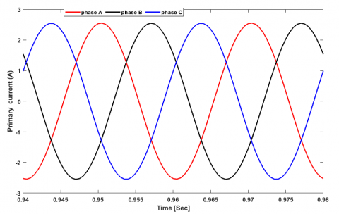
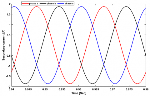
The primary is supplied with a sinusoidal voltage which has N1 continuous coils of n1 turns, so it absorbs a current shown in Figure 3 which represents the currents of the three phases on the high voltage side, the primary transforms electrokinetic energy into magnetic energy, the secondary has N2 coils made up of n2 turns, it transforms magnetic energy received from the primary into electrokinetic energy, Figure 4 represents the variation of currents in the secondary of the transformer. In sinusoidal regime, the voltages and currents are related to each other by the relation:
V1= (N1/N2) V2 and I1= (N2/N1) I2, V2=Z2 I2
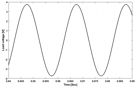
In a transformer, the voltage at the secondary varies according to the nature of the load, moreover in our case the load is a resistor so the voltage and the current are in phase, Figure 5 represents the voltage variation at the secondary.
Analysis of the different currents in healthy and faulty states in the presence of short-circuit inter-turns faults allows us to have quickly the signature of the different percentages of short-circuit inter-turns of a phase of the transformer, so we will proceed to different comparison, the results are presented below.In a transformer, the voltage at the secondary varies according to the nature of the load, moreover in our case the load is a resistor so the voltage and the current are in phase, Figure 5 represents the voltage variation at the secondary.
Figure 3. Primary currents in healthy state
Figure 4. Secondary currents in healthy state
Figure 5. Load voltage
Figure 6. Primary currents at 10% of short circuit turns
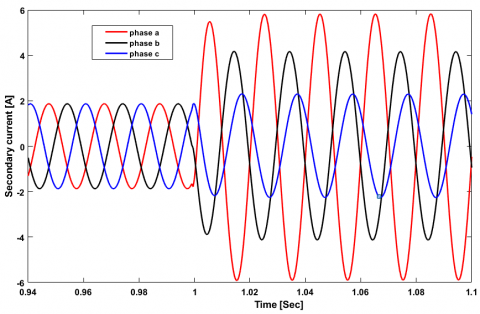
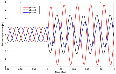
Figure 7. Secondary currents at 10% short circuit turns
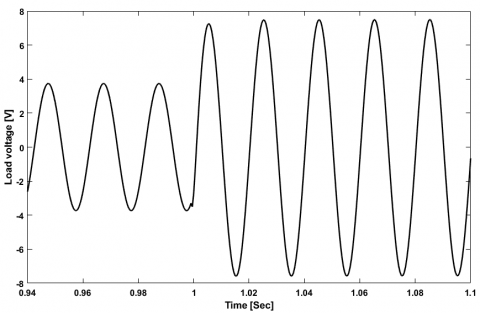
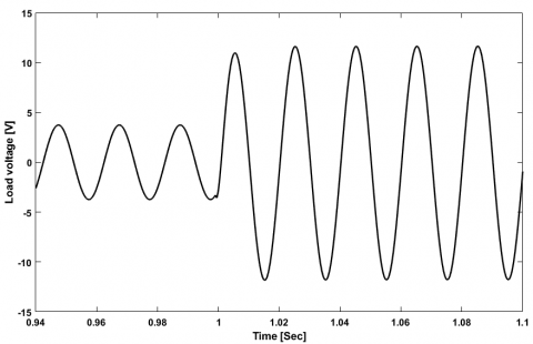
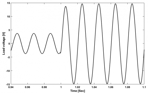
Figure 8. Load voltage at 10% short circuit turns
Figure 9. Primary currents at 20% of short circuit turns
Figure 10. Secondary currents at 20% short circuit turns
Figure 11. Load voltage at 20% short circuit turns
Figure 12. Primary currents at 30% of short circuit turns
Figure 13. Secondary currents at 30% short circuit turns
Figure 14. Load voltage at 30% short circuit turns
The inter-turn fault was applied at t=1 seconds on phase "A" of the transformer primary under load. During these tests, we introduced the fault progressively with different percentages representing the ratio between the shorted turns and the total number of turns, we took 10%, 20% and 30%. For each test we observed the evolution of the primary and secondary currents of the transformer as well as the load voltage. When a short circuit fault is applied between turns, it cancels the flow of the magnetic circuit in the faulted area, causing an abnormally high magnetizing current, and decreasing the winding resistance [17]. This is due to the fact that the electrical resistances of the turns of a given winding, which should be in series and isolated from each other, are placed in parallel, which causes an increase in the currents flowing through the three phases of the primary, the higher the percentage of fault, the greater the current in the faulty phase, as shown in Figures 6, 9 and 12. With the presence of the short circuit between turns in the primary which can appear at different places of the windings. When a short-circuit fault occurs, there is a current, called circulation current, which flows through the short-circuited windings. This current will also generate an electromagnetic field that will disturb the field transmitted to the secondary [18].
Generally, the effect of a short circuit is to disturb the distribution of the magnetic flux. On the one hand, this leads to oscillations in the secondary currents, on the other hand, the current flowing in the short-circuited turns can reach high values, resulting in an excessive increase of the current in the different phases of the secondary [19] as shown in Figures 7, 10 and 13. The variation of the load voltage is proportional to the secondary current, so an increase of the current causes an increase of the voltage for the same load, Figures 8, 11 and 14 represent respectively the load voltage when applying 10%, 20% and 30% of short circuit fault between turns.
Another technique for diagnosing faults in transformers in full operation is exploded and may be interesting. This method is based on monitoring the primary current as a function of the voltage drop across the secondary of the transformer at 50 Hz for different operating conditions.
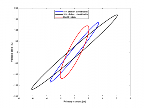
Figure 15 shows a comparison between the secondary voltage drop as a function of the primary current for different percentages of inter-turn short circuits and the healthy state.
Figure 15. Secondary voltage drop versus primary current
The relationship between the input current and the voltage drop is an ellipse. To control the transformer at full power, it is sufficient to monitor the angle of inclination of the ellipse. The angle of inclination is defined as the ratio between the height of the inner axis and the outer axis of the ellipse as given in Eq. (32):
$\sin \alpha=h / H$ (32)
In this paper, a presentation of the technique of modeling inter-turn short circuits by coupling magnetic circuits is developed. A thorough explanation of the cause of this failure is studied. Several scenarios of inter-turn short circuit faults have been applied. Two techniques for diagnosing these faults have been used: the state model and the voltage drop versus primary current. The results obtained demonstrate the accuracy of the mathematical model, which can be very useful for studying other types of faults. even the voltage drop versus current can be a means of monitoring the state of charge of the transformer on the one hand and its own state on the other. this technique does not require any specific hardware and can be implemented on-line as it is performed at the frequency of electrical networks.
|
Greek symbols |
|
|
$\alpha$ |
angle of inclination |
|
$\varphi$ |
magnetic flux |
|
µ |
permeability H/m |
|
$\mathfrak{R}$ |
magnetic reluctance |
[1] Liu, Z. (2015). Chapter 1 - Global energy development: The reality and challenges. Global Energy Interconnection, 1-64. https://doi.org/10.1016/B978-0-12-804405-6.00001-4
[2] Keitoue, S., Murat, I., Filipović-Grčić, B., Župan, A., Damjanović, I., Pavić, I. (2018). Lightning caused overvoltages on power transformers recorded by on-line transient overvoltage monitoring system. Journal of Energy: Energija, 67(2): 44-53.
[3] Li, J., Li, X., Du, L., Cao, M., Qian, G. (2016). An intelligent sensor for the ultra-high-frequency partial discharge online monitoring of power transformers. Energies, 9(5): 383. http://doi.org/10.3390/en9050383
[4] Fofana, I., Hadjadj, Y. (2018). Power transformer diagnostics, monitoring and design features. Energies, 11(12): 3248. http://doi.org/10.3390/en11123248
[5] Mharakurwa, E.T., Nyakoe, G.N., Akumu, A.O. (2019). Power transformer fault severity estimation based on dissolved gas analysis and energy of fault formation technique. Journal of Electrical and Computer Engineering, 2019: 9674054. https://doi.org/10.1155/2019/9674054
[6] Hussain, G.A., Kumpulainen, L., Klüss, J.V., Lehtonen, M., Kay, J.A. (2013). The smart solution for the prediction of slowly developing electrical faults in MV switchgear using partial discharge measurements. IEEE Transactions on Power Delivery, 28(4): 2309-2316. http://doi.org/10.1109/tpwrd.2013.2266440
[7] Bilal, H., Heraud, N., Sambatra, E.J.R. (2021). An experimental approach for detection and quantification of short-circuit on a doubly fed induction machine (DFIM) windings. Journal of Control, Automation and Electrical Systems, 32(4): 1123-1130. http://doi.org/10.1007/s40313-021-00733-w
[8] Singh, J., Singh, S., Singh, A. (2019). Distribution transformer failure modes, effects and criticality analysis (FMECA). Engineering Failure Analysis, 99: 180-191. https://doi.org/10.1016/j.engfailanal.2019.02.014
[9] Berzoy, A., Mohamed, A.A.S., Mohammed, O.A. (2016). Inter-turn short-circuit fault model for magnetically coupled circuits: A general study. In 2016 IEEE Industry Applications Society Annual Meeting, pp. 1-7. https://doi.org/10.1109/IAS.2016.7731866
[10] Zhang, H., Yang, B., Xu, W., Wang, S., Wang, G., Huangfu, Y., Zhang, J. (2013). Dynamic deformation analysis of power transformer windings in short-circuit fault by FEM. IEEE Transactions on Applied Superconductivity, 24(3): 1-4. https://doi.org/10.1109/TASC.2013.2285335
[11] Fan, R., Meliopoulos, A.S., Sun, L., Tan, Z., Liu, Y. (2016). Transformer inter-turn faults detection by dynamic state estimation method. In 2016 North American Power Symposium (NAPS), pp. 1-6. https://doi.org/10.1109/naps.2016.7747999
[12] Sayed, A., Aliprantis, D., Ge, H., Laskaris, K. (2021). Coupled finite element and extended-QD circuit induction machine model, Part I: Formulation. IEEE Transactions on Energy Conversion, 36(3): 2556-2564. https://doi.org/10.1109/tec.2021.3058802
[13] Kenmoe Fankem, E.D., Kendeg Onla, C.J., Xiaoyan, W., Dountio Tchioffo, A., Effa, J.Y. (2021). Modelling of brushless doubly fed reluctance machines based on reluctance network model. IET Electric Power Applications, 15(10): 1384-1398. https://doi.org/10.1049/elp2.12106
[14] Terron-Santiago, C., Martinez-Roman, J., Puche-Panadero, R., Sapena-Bano, A. (2021). A review of techniques used for induction machine fault modelling. Sensors, 21(14): 4855. https://doi.org/10.3390/s21144855
[15] NITU, M.C., DUTA, M. (2018). Calculation of surges transmitted between transformer windings using the coupled circuit model. In 2018 International Conference on Applied and Theoretical Electricity (ICATE), pp. 1-6. https://doi.org/10.1109/icate.2018.8551475
[16] Gholami, M., Hajipour, E., Vakilian, M. (2016). A single phase transformer equivalent circuit for accurate turn to turn fault modeling. In 2016 24th Iranian Conference on Electrical Engineering (ICEE), pp. 592-597. https://doi.org/10.1109/IranianCEE.2016.7585591
[17] Obeid, N.H., Boileau, T., Nahid-Mobarakeh, B. (2016). Modeling and diagnostic of incipient interturn faults for a three-phase permanent magnet synchronous motor. IEEE Transactions on Industry Applications, 52(5): 4426-4434. https://doi.org/10.1109/tia.2016.2581760
[18] Ullah, Z., Hur, J. (2018). A comprehensive review of winding short circuit fault and irreversible demagnetization fault detection in PM type machines. Energies, 11(12): 3309. https://doi.org/10.3390/en11123309
[19] Yang, C., Ding, Y., Qiu, H., Xiong, B. (2021). Analysis of turn-to-turn fault on split-winding transformer using coupled field-circuit approach. Processes, 9(8): 1314. https://doi.org/10.3390/pr9081314