Abdelhak Benheniche* | Farid Berrezzek
© 2021 IIETA. This article is published by IIETA and is licensed under the CC BY 4.0 license (http://creativecommons.org/licenses/by/4.0/).
OPEN ACCESS
The goal of this work is to propose a latest design of a rotor speed and rotor flux modulus control approach for an induction machine using a Backstepping corrector with an integral action. The advantage of the Backstepping Strategy is the ability to manage a nonlinear system. The Lyapunov theory has been used to ensure the system stability. To improve the controller robustness proprieties the integral action is used, despite the system uncertainties and the existence of external disturbances. The unavailable rotor flux is recovered by estimation of the rotor flux of the machine based on the integration of the stator voltage expressions. The simulation results illustrate the effectiveness of the proposed control scheme under load disturbances, rotor resistance variation and low and high speed.
induction motor, nonlinear control technique, integral backstepping control, flux estimator, Lyapunov stability
Compared to other electric machine types, the induction motor plays a crucial role in many industrial applications because of its excellent reliability, great robustness, less maintenance, robustness and low cost [1-3]. However, the control problem is more complex for induction motors, due to their multivariable and strongly nonlinear dynamics [4]. Also, physical parameter uncertainties, such as the variation of the rotor resistance with temperature, affect significantly the dynamics of the system, whereas the load torque strictly depends on the load type. In the majority of industrial applications, it is required to be able to control the speed of induction motor drives. Using linear system theory for controlling the induction machine can present limitations, especially in transient regimes [5]. On the other hand, using the PI controller induces many problems such as high overshoot, oscillation of speed and torque due to sudden load changes and external disturbances. This poor ability to manage the uncertainty of the system constitutes a major drawback which can lead to a degradation of the system performance.
A literature review shows that nonlinear pre-compensation can be used as a powerful method for controlling the induction machine based on the linearization technique [6, 7]. Nevertheless, the nonlinear part of the system must be neglected [5]. The first control techniques used for variable speeds are based on classical scalar control allows to ensure only basic performances [8]. In different applications, it is important to integrate new sophisticated controls as Field Oriented Control (FOC). This command, which was initiated in 1972, consists to make the behavior of the induction motor analogous to that of the DC motor [9, 10]. Its principle is based on the model of the asynchronous machine in a rotating reference frame and makes it possible to independently control the flux and the torque in a manner similar to the DC machine. In the literature, two types of vector control are possible: the first is called direct vector control, which requires the estimation of the position of the vector rotor flux (modulus and phase). However, the next type is named indirect vector control, which is characterized only by the estimation of the rotor flux [10]. Nonetheless the drawbacks of this technique essentially reside in the sensitivity to motor parametric variations and external load disturbances, especially according to the rotor resistance variation [11]. Knowing the calculation of the flux orientation angle is based on this resistance.
A small variation in this resistance can cause an error in the orientation of the rotating frame. In addition, the consequences can influent on the decoupling [10].
To overcome these problems, various nonlinear command techniques have been examined. Among these nonlinear control techniques that ensure high performance and global decoupling between the outputs to control whatever the path profile imposed for the machine; we can cite the technique of input-output feedback linearization presented by Hill [12]. This technique focuses on the differential geometry principle to convert a non-linear system into a linear system using a linearization state feedback with input-output decoupling. From there, we can apply the theory of linear systems [13, 14].
The study presented in Refs. [15] and [16] shows that passivity based control method is incapable to eliminate the non-linearity terms. However, it allows guarantying the stability of system, taking into account a damping part of the global energy of the system. Also, this method ensures the robustness control under the parameter uncertainties. Nevertheless, this method has some drawbacks [17, 18].
1) The necessary and sufficient conditions used to linearize the system can't be permanently ensured during the time;
2) Existence of singular points;
3) Complexity of the controller and heavy computing of the load.
The sliding mode control represents another technique for controlling the systems. In fact, it has high robustness proprieties and its design is easy. The main disadvantage of this technique is the chattering phenomenon. Due to high oscillations of frequency this phenomenon is appeared. The consequence of the chattering phenomenon is the dynamic instability of systems [6, 19].
Recently, the technique of Backstepping command has been extensively discussed and designed for the nonlinear control of nonlinear systems [11, 20, 21]. This technique is initiated by Fateh and Abdellatif [20]. In transient and steady state regimes, this technique accords good performances. It’s considered more robust under the variations in parameter and presence of load torque perturbations. But it is relatively well in steady state regime. Indeed, the classical Backstepping control technique focuses on a proportional derivative, which provides a static error [20]. The conception of this method is realized by using Lyapunov stability tools. The modification of Backstepping approach of control by adding integral action is an interesting solution to improve the robustness of Backstepping control and eliminate residual errors [20].
The importance of the integral backstepping strategy in the control of induction motors by making a judicious choice of the Lyapunov function lies in the stability of the whole system [21]. The main advantages of this strategy of control are: robustness under parametric variation constraints and good tracking references [20].
In the present paper, the Backstepping approach control, robustness of speed-flux and torque $\left(\xi_{1}=\frac{1}{j} T_{e}\right)$ controllers have been improved by integrating new integral terms. The addition of the integral action makes it possible to significantly reduce the effect of the variation in resistance of the rotor as well as the disturbance due to the load torque and therefore eliminates the error in steady state.
The organization of this manuscript is given as follows: In section two the nonlinear induction motor model is presented. In section three, design of integral Back-stepping speed and flux controllers are developed. Estimator of rotor flux is presented in the section four. Finally, simulation results and interpretations are discussed.
To lower the multiplicity of the IM model, an equivalent representation of two phases has been used. This representation considers linearity assumptions of the magnetic circuit and neglects iron losses. The design of this model class is developed under the fixed $(\alpha, \beta)$ stator reference frame, by the following non-linear functions with the stator current, rotor flux and rotor speed as selected state variables of the motor. Under these conditions, the non-linear model of the IM can be formulated as follow [5]:
$\dot{x}=f(x)+g(x) u$ (1)
$y=h(x)$ (2)
With,
$f(x)=\left[\begin{array}{c}-\gamma i_{s \alpha}+\frac{K}{T_{r}} \varphi_{r \alpha}+p \omega \varphi_{r \beta} \\ -\gamma i_{s \beta}-p \omega K \varphi_{r \alpha}+\frac{K}{T_{r}} \varphi_{r \beta} \\ \frac{M}{T_{r}} i_{s \alpha}-\frac{1}{T_{r}} \varphi_{r \alpha}+p \omega \varphi_{r \beta} \\ \frac{M}{T_{r}} i_{s \beta}-p \omega \varphi_{r \alpha}-\frac{1}{T_{r}} \varphi_{r \beta} \\ \frac{p M}{j L_{x}}\left(\varphi_{r \alpha} i_{s \beta}-\varphi_{r \beta} i_{s \alpha}\right)-\frac{f}{j} \Omega-\frac{T_{l}}{i}\end{array}\right]$ (3)
$g(x)=\left[\begin{array}{llll}\frac{1}{\sigma L_{s}} & 0 & 0 & 0 \\ 0 & \frac{1}{\sigma L_{\mathrm{s}}} & 0 & 0\end{array}\right]^{T}$ (4)
$h(x)=\left[\begin{array}{llll}1 & 0 & 0 & 0 \\ 0 & 1 & 0 & 0\end{array}\right]$ (5)
$K=\frac{1}{M}\left(\frac{1-\sigma}{\sigma}\right), \sigma=1-\frac{M^{2}}{L_{s} L_{r}}, \gamma=\frac{1}{\sigma}\left(\frac{1}{T_{s}}+\frac{1-\sigma}{T_{r}}\right), \quad k_{f}=\frac{f}{j}$, $k_{l}=\frac{p}{j}$, and $\omega=p \Omega$
where,
3.1 Control objective
The goal of control is to design the virtual control (appropriate functions), to simplify a complex nonlinear control problem. The simplification has been done by dividing the control design into several steps. Each step deal with a single input-output design problem, and considered as a reference for the next step. To ensure global system stability and tracking objectives, the ELF is used step by step [21].
3.2 Step one
In this step, it is important to identify the target trajectories that the system must follow them. Also, to guarantee best tracking precision, the controllers must be designed.
The desired trajectories of rotor speed and rotor flux modulus are defined by $\Omega_{d}$ and $\varphi_{d}^{2}$.
The speed tracking error e1 and the flux modulus tracking error e3 can be controlled using the auxiliary variables $\xi_{1}^{d}$ and $\xi_{2}^{d}$ respectively.
We define tracking errors as:
$e_{1}=\Omega_{d}-\Omega$ (6)
$e_{3}=\psi_{d}-\psi_{r}$ (7)
With $\psi_{r}=\varphi_{r \alpha}^{2}+\varphi_{r \beta}^{2}$.
Their dynamics equations are given by:
$\dot{e}_{1}=\dot{\Omega}_{d}-\left[\frac{p M}{j L_{r}}\left(\varphi_{r \alpha} \dot{i}_{s \beta}-\varphi_{r \beta} i_{s \alpha}\right)-\frac{T_{l}}{j}-\frac{f}{j} \Omega\right]$ (8)
$\dot{e}_{3}=\psi_{d}-\left[\frac{2 M}{T_{r}}\left(\varphi_{r \alpha} i_{s \alpha}+\varphi_{r \beta} i_{s \beta}\right)\right]+\frac{2}{T_{r}} \psi_{r}$ (9)
The virtual control expressions are given as follow:
$\xi_{1}=\left[\frac{p M}{j L_{r}}\left(\varphi_{r \alpha} i_{s \beta}-\varphi_{r \beta} i_{s \alpha}\right)\right]$ (10)
$\xi_{2}=\left[\frac{2 M}{T_{r}}\left(\varphi_{r \alpha} i_{s \alpha}+\varphi_{r \beta} i_{s \beta}\right)\right]$ (11)
Eqns. (8) and (9) can be formulated by the following expressions:
$\dot{e}_{1}=\dot{\Omega}_{d}-\xi_{1}+\frac{T_{l}}{j}+\frac{f}{j} \Omega$ (12)
$\dot{e}_{3}=\dot{\psi}_{d}-\xi_{2}+\frac{2}{T_{r}} \varphi_{r}^{2}$ (13)
Checking of the tracking error dynamics stability is based on the following CLF:
$v_{1}=\frac{1}{2}\left[e_{1}^{2}+e_{3}^{2}\right]$ (14)
The mathematical expression given in (15) shows a derivative of (14) in a function of time.
$\dot{v}_{1}=e_{1} \dot{e}_{1}+e_{3} \dot{e}_{3}$ (15)
The derivative error tracking has been chosen as follows.
$\dot{e}_{1}=-k_{1} e_{1}$ (16)
$\dot{e}_{3}=-k_{3} e_{3}$ (17)
The negative sign of (16) and (17) means that Lyapunov function is negative defined.
So, under these conditions, the virtual control extracted from expressions (12) and (13) can be written as follow:
$\xi_{1}^{*}=k_{1} e_{1}+\dot{\Omega}_{d}+\frac{T_{l}}{j}+\frac{f}{j} \Omega$ (18)
$\xi_{2}^{*}=k_{3} e_{3}+\dot{\psi}_{d}+\frac{2}{T_{r}}\left(\psi_{d}-e_{3}\right)$ (19)
where, coefficients k1 and k3 represent the positive design gains that define the dynamic of closed loop.
The derivative of the LF according to time is clearly negative definite. Then the tracking error e1 and e3 can reach a permanent regime.
Since the variables $\xi_{1}$ and $\xi_{2}$ are not a control inputs and only two variables of the system with its own dynamics. We will utilize it to insert the integral action, so the virtual controls $\xi_{1}^{*}$ and $\xi_{2}^{*}$ are used to guarantee the stability of the speed and modulus flux loops. The dynamics of the tracking errors are given by:
$\xi_{1}^{d}=\xi_{1}^{*}+\lambda_{1} \chi_{1}$ (20)
$\xi_{2}^{d}=\xi_{2}^{*}+\lambda_{2} \chi_{2}$ (21)
With $\lambda_{1}$ and $\lambda_{2}$ are positive constants and $\chi_{i}=\int_{0}^{t} e_{i}(\tau) d \tau \quad i=1,2$ are the integral actions brought in accordance with the following error. By introducing there in the virtual control, we insure the convergence of the error towards zero in steady state.
3.3 Step two
The control objective becomes: oblige the auxiliary variable $\xi_{1}$ to track $\xi_{1}^{d}$ while $\xi_{2}$ must track $\xi_{2}^{d}$.
Last references have been chosen to guarantee a steady dynamic of velocity and flux modulus tracking error. Considering errors between them is important for virtual controls. The control objective becomes: force the auxiliary variable $\xi_{1}$ to track $\xi_{1}^{d}$ while $\xi_{2}$ must track $\xi_{2}^{d}$.
To this end, let us define the following errors:
$e_{2}=\xi_{1}^{d}-\xi_{1}=\xi_{1}^{*}+\lambda_{1} \chi_{1}-\xi_{1}$ (22)
$e_{4}=\xi_{2}^{d}-\xi_{2}=\xi_{2}^{*}+\lambda_{2} \chi_{2}-\xi_{2}$ (23)
The time derivative of (22) and (23) gives:
$\dot{e}_{2}=\dot{\xi}_{1}^{d}-\dot{\xi}_{1}=\xi_{1}^{*}+\lambda_{1} e_{1}-\dot{\xi}_{1}$ (24)
$\dot{e}_{4}=\dot{\xi}_{2}^{d}-\dot{\xi}_{2}=\dot{\xi}_{2}^{*}+\lambda_{2} e_{3}-\dot{\xi}_{2}$ (25)
New formulation of equations (24) and (25) in function of new terms e2 and e4 are given as follow:
$\dot{e}_{1}=-k_{1} e_{1}+e_{2}$ (26)
$\dot{e}_{3}=-k_{3} e_{3}+e_{4}$ (27)
From (24) and (25), new formulations of error dynamics have been obtained.
$\dot{e}_{2}=\xi_{3}-\left[\frac{p K}{j}\left(\varphi_{r \alpha} u_{s \beta}-\varphi_{r \beta} u_{s \alpha}\right)\right]$ (28)
$\dot{e}_{4}=\xi_{4}-\left[2 K R_{r}\left(\varphi_{r \alpha} u_{s \alpha}+\varphi_{r \beta} u_{s \beta}\right)\right]$ (29)
where,
$\xi_{3}=\dot{\xi}_{1}^{d}+\frac{p M}{j L_{r}}\left[\left(\gamma+\frac{1}{T_{r}}\right)\left(\varphi_{r \alpha} i_{s \beta}-\varphi_{r \beta} i_{s \alpha}\right)\right]$
$+\frac{p M}{j L_{r}}\left[p \Omega\left[\left(\varphi_{r \alpha} i_{s \alpha}+\varphi_{r \beta} i_{s \beta}\right)+K \varphi_{r}^{2}\right]\right]$
$\xi_{4}=\dot{\xi}_{2}^{d}+\frac{2 M}{T_{r}}\left[\left(\gamma+\frac{1}{T_{r}}\right)\left(\varphi_{r \alpha} i_{s \alpha}+\varphi_{r \beta} i_{s \beta}\right)-\frac{K}{T_{r}} \varphi_{r}^{2}\right]$
$-\frac{2 M}{T_{r}}\left[p \Omega\left(\varphi_{r \alpha} i_{s \beta}-\varphi_{r \beta} i_{s \alpha}\right)\right.$
$\left.+\frac{M}{T_{r}}\left(i_{s \alpha}^{2}+i_{s \beta}^{2}\right)\right]$
Expressions (28) and (29) show that the control term is included in the error dynamics formulations. So, the development of the augmented Lyapunov function is evident. Relation (30) shows this function.
$v_{2}=\frac{1}{2}\left[e_{1}^{2}+e_{2}^{2}+e_{3}^{2}+e_{4}^{2}\right]$ (30)
Calculating the derivative of equation (30) we obtain:
$\dot{v}_{2}=-k_{1} e_{1}^{2}+e_{1} e_{2}-k_{3} e_{3}^{2}+e_{3} e_{4}-k_{2} e_{2}^{2}-$
$k_{4} e_{4}^{2}+e_{2}\left(k_{2} e_{2}+e_{1}+\xi_{3}+\frac{p K}{j}\left(\varphi_{r \alpha} u_{s \beta}-\right.\right.$
$\left.\left.\varphi_{r \beta} u_{s \alpha}\right)\right)+e_{4}\left(k_{4} e_{4}+e_{3}+\xi_{4}-\right.$
$\left.2 K R_{r}\left[2 K R_{r}\left(\varphi_{r \alpha} u_{s \alpha}+\varphi_{r \beta} u_{s \beta}\right)\right]\right)$ (31)
where k2 and k4 are the positive constant that determine the dynamic of closed loop.
To ensure the CLF derivative semi-negative definite, it is important to find the following expression:
$\dot{v}_{2}=-k_{1} e_{1}^{2}-k_{3} e_{3}^{2}-k_{2} e_{2}^{2}-k_{4} e_{4}^{2} \leq 0$ (32)
The voltage control has been chosen as follow:
$k_{2} e_{2}+e_{1}+\xi_{3}+\frac{p K}{j}\left(\varphi_{r \alpha} u_{s \beta}-\varphi_{r \beta} u_{s \alpha}\right)=0$ (33)
$k_{4} e_{4}+e_{3}+\xi_{4}-2 K R_{r}\left(\varphi_{r \alpha} u_{s \alpha}+\varphi_{r \beta} u_{s \beta}\right)=0$ (34)
So, the obtained control expressions are given as follow:
$u_{s \alpha}=\frac{1}{\psi_{r}}\left[\frac{\left(\xi_{4}+e_{3}+k_{4} e_{4}\right)}{2 K R_{r}} \varphi_{r \alpha}-\frac{j}{p K}\left[\xi_{3}+e_{1}+k_{2} e_{2}\right] \varphi_{r \beta}\right]$ (35)
$u_{s \beta}=\frac{1}{\psi_{r}}\left[\frac{\left(\xi_{4}+e_{3}+k_{4} e_{4}\right)}{2 K R_{r}} \varphi_{r \beta}+\frac{j}{p K}\left[\xi_{3}+e_{1}+k_{2} e_{2}\right] \varphi_{r \alpha}\right]$ (36)
3.4 Rotor flux estimator
So that the rotor flux is estimated, many methods founded on open loop observers can be used. To show the effectiveness of the proposed control approach, the rotor flux estimator has been used. The estimator using the stator voltage expressions in the stationary frame $(\alpha, \beta)$ has been used. The estimator developed can be extracted from the following equations [22]:
$\dot{\hat{\varphi}}_{r \alpha}=\frac{L_{r}}{M} u_{s \alpha}-\frac{L_{r}}{M}\left(R_{s}+\sigma L_{s} \frac{d}{d t}\right) i_{s \alpha}$ (37)
$\dot{\hat{\varphi}}_{r \beta}=\frac{L_{r}}{M} u_{s \beta}-\frac{L_{r}}{M}\left(R_{s}+\sigma L_{s} \frac{d}{d t}\right) i_{s \beta}$ (38)
$\hat{\psi}_{r}=\hat{\varphi}_{r \alpha}^{2}+\hat{\varphi}_{r \beta}^{2}$ (39)
where, $\left(\varphi_{r \alpha}, \varphi_{r \beta}\right)$ are the estimated rotor flux components and $\left(i_{s \alpha}, i_{s \beta}\right)$ are the stator measured stator current components.
To illustrate the advantages of the proposed integral Backstepping, an induction machine with its proper characteristics is considered as presented in Table 1.
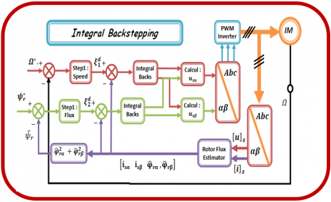
The simulation block diagram of the Backstepping control combined with an integral action approach of the induction motor model is given in Figure 1. In this work the simulation tests were carried out using Matlab software.
Two steps are necessary to carry out the simulation of the proposed scheme.
Table 1. Induction motor characteristics
|
Nomination |
Definition |
Numerical Values |
|
Pa |
Nominal Power |
1.5 KW |
|
F |
Operating frequency |
50 HZ |
|
P |
Pair pole number |
2 |
|
U |
Supply |
220 V |
|
Rs |
Stator resistance |
4.850 $\Omega$ |
|
Rr |
Rotor resistance |
3.805 $\Omega$ |
|
Ls |
Stator inductance |
0.274 H |
|
Lr |
Rotor inductance |
0.274 H |
|
M |
Mutual inductance |
0.258 H |
|
$\omega$ |
Rotor angular velocity |
297.25 rd/s |
|
J |
Inertia coefficient |
0.0031 Kg2/s |
|
f |
Friction coefficient |
0.00114 N.s/rd |
|
Tl |
Load Torque |
5 N.m |
Figure 1. Simulated bloc diagram of the proposed control
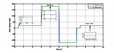
In the simulation section, the obtained results and discussions are given. Simulation results given by Figure 2 to Figure 6 demonstrate variations of the measured state variable of the motor and, reference signal in function of load variation. Between [4 sec-6 sec], the load is introduced by a value of $T_{l}=5 N . m$, and rotor resistance $R_{r}=1.5 * R_{r}$ introduced at 8.5 sec.
This simulation is realized by considering a reference speed as given in Figure 2. This reference is changed from 0 rd/s to 20 rd/s, to 180 rd/s then reversed to -120 rd/s, then reverted to 0 rd/s, then 20 rd/s at t=0.4 sec, 3 sec, 5 sec, 7 sec and 7.4 sec, respectively. Moreover, the motor is loaded suddenly between [4 sec-6 sec]. From this variation profile; we can notice that the measured speed converges perfectly towards its reference.
Figure 2. Reference and measured evolution of Rotor speed according to $T_{l}$ and $R_{r}$ variations
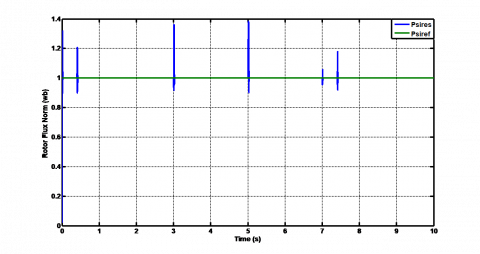
Figure 3. Reference and measured of the rotor flux norm under $T_{l}$ and $R_{r}$ variations
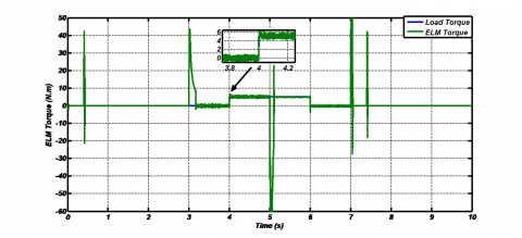
Figure 4. Variation of load and measured electromechanical torque
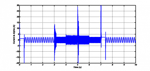
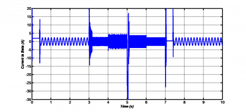
Figure 5. Measured $(\alpha-\beta)$ stator currents
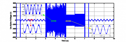
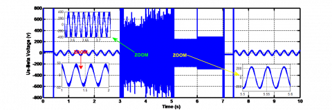
Figure 6. $(\alpha-\beta)$ stator voltage control inputs
Figure 3 illustrates that measured rotor flux norm follows the imposed flux with some disruption (peaks) when the speed change, the load and electromechanically torque of the motor are portrayed in Figure 4. A better tracking with negligible steady state error and a quick convergence, Figures 5-6 show respectively the measured stator currents and stator voltage components. Also, the simulation tests demonstrates that a remarkable decoupling impact of flux and torque components under rotor velocity, torque of load and rotor resistance variations, but the curves of rotor flux modulus, stator currents, torque and stator voltage present a peak when the speed change. This peak appeared because the specific action of the PWM inverter.
A new control scheme has been proposed in this manuscript. The proposed technique based on Backstepping control strategy with integration of integral action. The presented control combined with estimator have been tested via simulation under different operating conditions of the motor, specifically under conditions of load and speed variations, at low and high speed with a dynamic variation in rotor resistance of the motor.
The obtained results demonstrate that the proposed approach of control has high performances and ensures a perfect decoupling between the torque and flux. In fact, the machine operates permanently under these performances. Furthermore, by considering online parameter estimation the proposed approach can be improved.
Moreover, the obtained simulation results explain that the developed approach able to improve the performance of trajectory tracking under different conditions. In the case of nonlinear control, the use of estimator considered efficient tool to estimate the states of unmeasurable variables (rotor flux). As perspectives for future works, experimental tests are envisaged.
[1] Bensaker, B., Kherfane, H., Maouche, A., Metatla, A., Wamkeue, R. (2004). Sensorless monitoring of induction motor drive systems. IFAC Proceedings Volumes, 37(15): 89-94. https://doi.org/10.1016/S1474-6670(17)31005-4
[2] Dos Santos, T.H., Goedtel, A., Da Silva, S.A.O., Suetake, M. (2014). Scalar control of an induction motor using a neural sensorless technique. Electric Power Systems Research, 108: 322-330. https://doi.org/10.1016/j.epsr.2013.11.020
[3] Fathabadi, F.R., Molavi, A. (2019). Black-box identification and validation of an induction motor in an experimental application. European Journal of Electrical Engineering, 21(2): 255-263. https://doi.org/10.18280/ejee.210219
[4] Mohamed, H., Lotfi, B. (2020). Improvement of direct torque control performances for induction machine using a robust backstepping controller and a new stator resistance compensator. European Journal of Electrical Engineering, 22(2): 137-144. https://doi.org/10.18280/ejee.220207
[5] Berrezzek, F., Bourbia, W., Bensaker, B. (2019). A comparative study of nonlinear circle criterion based observer and H∞ observer for induction motor drive. Int. J. Power Electron. Drive Syst., 10(3); 1229-1243.
[6] Utkin, V.I. (1993). Sliding mode control design principles and applications to electric drives. IEEE Trans. Ind. Electron., 40(1): 23-36. https://doi.org/10.1109/41.184818
[7] Lee, H.T., Fu, L.C., Lu, F.L, (2006). Sensorless adaptive backstepping speed control of induction motor. Proceedings of the 45th IEEE Conference on Decision & Control, San Diego, CA, USA, pp. 1252-1257. https://doi.org/10.1109/CDC.2006.377160
[8] Mehazzem, F., Nemmour, A.L., Reama, A., Benalla, H. (2011). Nonlinear integral backstepping control for induction motors. International Aegean Conference on Electrical Machines and Power Electronics and Electromotion, Joint Conference, pp. 331-336. https://doi.org/10.1109/ACEMP.2011.6490619
[9] Ammar, A., Kheldoun, A., Metidji, B., Ameid, T., Azzoug, Y. (2020). Feedback linearization based sensorless direct torque control using stator flux MRAS-sliding mode observer for induction motor drive. ISA Transactions, 98: 382-392. https://doi.org/10.1016/j.isatra.2019.08.061
[10] Lima, F., Kaiser, W., Da Silva, I.N., De Oliveira, A.A.A. (2014). Open-loop neuro-fuzzy speed estimator applied to vector and scalar induction motor drives. Applied Soft Computing, 21: 469-480. https://doi.org/10.1016/j.asoc.2014.03.044
[11] Trabelsi, R., Khedher, A., Mimouni, M.F., M’Sahli, F. (2012). Backstepping control for an induction motor using an adaptive sliding rotor-flux observer. Electric Power Systems Research, 93: 1-15. https://doi.org/10.1016/j.epsr.2012.06.004
[12] Hill, D.J. (1987). Nonlinear control systems: An introduction. A. Isidori. Automatica, 23(3): 415-416. https://doi.org/10.1016/0005-1098(87)90019-7
[13] Oukaci, A., Toufouti, R., Dib, D., Atarsia, L. (2017). Comparison performance between sliding mode control and nonlinear control, application to induction motor. Electrical Engineering, 99(1): 33-45. https://doi.org/10.1007/s00202-016-0376-3
[14] Farid, B., Wafa, B., Bachir, B. (2013). Nonlinear control of induction motor: A combination of nonlinear observer design and input-output linearization technique. Journal of Power and Energy Engineering, 7: 1001-1008.
[15] Abdel Fattah, H.A., Loparo, K.A. (2003). Passivity-based torque and flux tracking for induction motors with magnetic saturation. Automatica, 39(12): 2123-2130. https://doi.org/10.1016/S0005-1098(03)00251-6
[16] Shiau, L.G., Lin, J.L., Yeh, Y.J. (2001). Passivity based control for induction motor drives with voltage-fed. Electric Power Systems Research, 59(1): 1-11. https://doi.org/10.1016/S0378-7796(01)00135-3
[17] Chen, F., Xu, W. (1999). Passivity-based speed control (PBC) of induction motor. IFAC Proceedings Volumes, 32(2): 2164-2168. https://doi.org/10.1016/s1474-6670(17)56367-3
[18] Kumar, A., Shanmugavadivu, P. (2019). Skin Detection Using Hybrid Colour Space of RGB-H-CMYK. In: Pati B., Panigrahi C., Misra S., Pujari A., Bakshi S. (eds) Progress in Advanced Computing and Intelligent Engineering. Advances in Intelligent Systems and Computing, vol 713. Springer, Singapore. https://doi.org/10.1007/978-981-13-1708-8_7
[19] Oliveira, C.M.R., Aguiar, M.L., Monteiro, J.R.B.A., Pereira, W.C.A., Paula, G.T., Almeida, T.E.P. (2016). Vector control of induction motor using an integral sliding mode controller with anti-windup. Journal of Control, Automation and Electrical Systems, 27(2): 169-178. https://doi.org/10.1007/s40313-016-0228-4
[20] Fateh, M., Abdellatif, R. (2017). Comparative study of integral and classical backstepping controllers in IFOC of induction motor fed by voltage source inverter. International Journal of Hydrogen Energy, 42(28): 17953-17964. https://doi.org/10.1016/j.ijhydene.2017.04.292
[21] Mehazzem, F., Nemmour, A.L., Reama, A. (2017). Real time implementation of backstepping-multiscalar control to induction motor fed by voltage source inverter. International Journal of Hydrogen Energy, 42(28): 17965-17975. https://doi.org/10.1016/j.ijhydene.2017.05.035
[22] Abid, M, Aissaoui, A.G. (2008). Fuzzy sliding mode control of an induction machine. Acta Electrotehnica, 49(2): 138-146.