Takieddine Meriouma* | Sid Ahmed Bessedik | Rabah Djekidel
© 2021 IIETA. This article is published by IIETA and is licensed under the CC BY 4.0 license (http://creativecommons.org/licenses/by/4.0/).
OPEN ACCESS
To meet the needs for electrical energy consumption, an increasing number of overhead high-voltage (HV) power lines are being installed, which raises public concern about the possible effects on health and environment. Therefore, it is very important to determine the exact exposure to electromagnetic fields at industrial frequency. This paper presents a two-dimensional (2D) numerical model for the electric field and magnetic induction radiated by a 400 kV overhead power line. The model adopts novel optimization methodologies based on cutting-edge simulation methods combined with the Evolutionary algorithms (EAs), such as the Krill Herd Algorithm (KH) and the grasshopper optimization algorithm (GOA) to solve the numerical optimization problems. The obtained maximum values of electric field and magnetic induction were below the limits for occupational and general public exposure set by the International Commission on Non-Ionizing Radiation Protection (ICNIRP). Finally, the obtained simulation results were found to agree well with those gained from the COMSOL Multiphysics 4.3b. To confirm the effectiveness of the proposed hybrid methods, the results obtained are also verified with measurement values available in the literature, and a good correlation is achieved.
charge simulation method (CSM), current simulation technique (CST), electric field, magnetic induction, krill herd algorithm (KH), grasshopper optimization algorithm (GOA), COMSOL Multiphysics 4.3b
Population growth and economic expansion have pushed up the global demand for electric energy, which calls for more energy transport infrastructures, e.g., overhead power lines and underground cables with high voltage levels. The development of these infrastructures generates and intensifies the interactions and electromagnetic problems, bringing more environmental and health risks [1, 2].
In recent years, the International Commission on Non-Ionizing Radiation Protection (ICNIRP) and many other international health institutions and organizations paid attention to the human health effects of the exposure to low frequency (LF) electric and magnetic fields emitted by high-voltage (HV) overhead power lines [1-10]. The potential hazard of this exposure represents a public and environmental concern. To disclose the possible health effects, it is critical to compute the Extremely low frequency (ELF) electric and magnetic fields in a precise manner.
Concerning human safety, many countries adopt the permissible levels on possible human exposure to magnetic and electric fields specified by the International Commission on Non-Ionizing Radiation Protection (ICNIRP) guidelines for occupational and general public exposure. The latest permissible exposure levels are set at 50-Hz extremely low frequency: For magnetic induction, the levels are 1 mT for occupational public, and 200 μT for the general public; for electric field, the levels are 10 kV/m for occupational public, and 5 kV/m for the general public. The ICNIRP also sets a limit on current density to a value of 10 mA/m2 [11].
Generally, in accordance with the quasi-static approximation of Maxwell equations, the resolution of electric and magnetic fields is simplified into static forms following Laplace's equations, which are solved using satisfied Dirichlet-type boundary conditions by various numerical methods.
Through two-dimensional (2D) approximation, this paper presents numerical methods for the electric and magnetic fields analysis created by the HV overhead power lines. The computation methodologies were designed based on the charge simulation method (CSM) and the current simulation technique (CST). To solve the main drawbacks of the parameters optimization required to these methods calculation, consisting in number and position of the fictitious charges and the filament line currents for a precise calculation, the Evolutionary Algorithms (EAs) have become a well recognized population meta-heuristic to solve the multiple constraints. And based on that, the KH algorithm and the GOA were applied. The obtained simulation results were compared to those resulting from the COMSOL Multiphysics 4.3b software, which is based on the finite element method (FEM). To confirm the high computation accuracy of these combined methods, a comparison is made with the measured values available in the literature [12].
2.1 Charge Simulation Method (CSM)
The procedure for determining the electrostatic field is generally to solve the Laplace equation with appropriate boundary conditions of Dirichlet problem, where the Laplace's equation is satisfied in the region S under consideration, as shown below [13]:
∇2V(s)=0,s∈S (1)
And the boundary condition of Dirichlet is satisfied on the boundary Γ:
V(s)=f(s),s∈Γ (2)
where, ∇2 is the Laplacian operator and s is the location. In the electrostatic field problem, v is generally taken as the electric potential and Γ is generally taken as the surfaces of conductors [13].
In this analysis, the charge simulation method (CSM) is applied to obtain an approximate solution of the Laplace equation, which is a method that belongs to the family of integral methods.
The principle of this method is based that the real surface charges on the surface of conductors are simulated and replaced by a set of fictitious discrete charges, which are properly arranged within the conductors [13-18].
The charge magnitudes must be calculated to satisfy the Dirichlet boundary conditions on an exact number of selected contour points. After determining the values of fictitious charges, it is possible to readily compute the potential and electric field distribution anywhere in the region. According to the superposition theorem, let qj be a number of n individual charges and Vi be the potential at any point within the space can be calculated as follows [13-18]:
Vi=n∑j=1Pij.qj (3)
where, Pij is the potential coefficient related to the potential of the jthcharge at the ith contour point, qjis the fictitious charges, n is the number of fictitious charges.
Then, the magnitude of fictitious charge can be determined by solving the system of nlinear equations as described below in Eq. (4) [13-18]:
[qj]n×n=[Pij]−1n×[Vi]n (4)
where, [Pij]is the potential coefficient matrix; [qi] is the column vector of values of unknown charge; [Vi] is the column vector of the voltage applied to contour points on the surface of conductors.
Once the values of fictitious charges are determined, it is possible to calculate the electric field intensity at any point around the conductors. The horizontal and vertical components of the electric field due to the total fictitious charges and their images for a Cartesian coordinate system at any point in space can be expressed by the following equations [13-18]:
Exi=NT∑j=1fxi.qjEyi=NT∑j=1fyi.qj} (5)
where, fxi,fyiare the coefficients of the electric field intensity between the contour points and the fictitious charges qj, which can be obtained using the following equations:
fxi=(12.π.ε0).((x−xj)(x−xj)2+(y−yj)2−(x−xj)(x−xj)2+(y+yj)2)fyi=(12.π.ε0).((y−yj)(x−xj)2+(y−yj)2−(y+yj)(x−xj)2+(y+yj)2)} (6)
where, (x,y) are the coordinates of the observation point; (xj,yj) are the coordinates of the fictitious charges.
Finally, when the two components are determined, it is possible to calculate the resultant of the electric field at any desired point by adding these components, as follows [13-18].
Eres=√E2xi+E2yi (7)
2.2 Current simulation technique (CST)
In the same manner of the electrostatic field, the magnetic induction can be obtained by the general solution of the magnetic scalar potential represented by the Laplace’s equation in a region k of space, with suitable boundary conditions for magnetic scalar potential ϕk at the border of the region k similar to the boundary conditions levied on the electrostatic potential problem, as shown below [19]:
∇2ϕk=0 (8)
where, ϕk is the Magnetic scalar potential; ∇2is the Laplacian operator.
Many resolution methods are available for magnetic induction calculation from HV power lines. Similar to the charge simulation method (CSM) principle, the current simulation technique (CST) treats each sub-conductor current as a finite number nf of filament line currents, which are distributed on a fictitious cylindrical surface of radius Rj. The number and coordinates of the simulation currents are not arbitrary but based on the number of conductors and their spatial arrangement [20-23].
For all number of filament line currents, the simulation currents along all sub-conductors Ii (i = 1…....3×nf×m) must meet the following conditions [20-23]:
(1) The component of the magnetic field intensity must be zero on the surfaces of the sub-conductors following the Biot-Savart law.
(2) The current of a sub-conductor must be equal to the sum of the filament line currents, which simulate that current.
Aij=3.nf.m∑i=1Kij.Ii=0,j=1,2,3,........,3.m.(nf−1) (9)
nf.q∑i=(q−1).nf+1Ii=Icq,q=1,2,3,..............,3.m (10)
where, m is the number of sub-conductors per phase; nf is the number of filament line currents.
After several contour points are selected from the surface of sub-conductors, the unknown filament currents can be determined by a set of equations [20-23]:
Kij=μ02πlnRjRij (11)
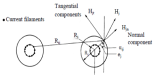
where, Kijis the coefficient of normal magnetic field specified by the coordinates of the ithcontour point; the jth filament line current is given by [20-23];Rijis the distance between simulation current point j and match pointi, Rjis the fictitious radius of current filament simulation (see Figure 1).
Figure 1. Normal and tangential field components at a point on the sub-conductor surface
After the unknown filament line currents are solved by the set of Eqns. (9) and (10), the horizontal and vertical components of the magnetic induction can be determined by:
Bxi=∂Aij∂xByi=∂Aij∂y} (12)
where, Aijis the magnetic vector generated by the three-phase power line conductors current, it’s expressed as follows [20-23]:
Aij=μ02.π3.n.m∑i=1Ii.Kij (13)
For the calculation of the magnetic field, the image of the filament line current in each sub-conductor is located at a penetration depth De different from the height of the sub-conductor above ground, and is given by [20-23]:
De=√2.√(ρ/π.μ0.f).e−jπ/4 (14)
where,ρ is the electrical resistivity of the medium; f is the frequency of the source current; μ0 is the permeability of free space.
The intensity of the resultant magnetic induction can be calculated by adding up the horizontal and vertical components mentioned above in Eq. (12) [20-23]:
Br=√B2xj+B2yj (15)
Taking into account the effect of the earth wires, the induced currents circulating in these earth wires can be solved by the Gaussian method, as shown in the following equation [24-26]:
[Ig]=- [Z−1ii]. [Zik].[Ic] (16)
where, Zii is the matrix of mutual impedances between phase conductors and earth wires; Zik is the matrix of self-impedance of the earth wires; Ic is the matrix of currents passing through the phase conductors.
At low frequencies, the mutual and self-longitudinal impedances with earth return of the conductors can be obtained by Carson-Clem’s formula [24-26]:
Zii=Ri+μ0.ω8+j.μ0.ω2.π.[ln(DeRGM)] (17)
Zik=μ0.ω8+j.μ0.ω2.π.ln(Dedik) (18)
where, Ri is the DC resistance per unit length of conductor in (Ω/km), RGM is the geometric mean radius of the conductor in (m); dik is the distance between the conductor i and the conductor kin (m); ω is the angular frequency (rad/s); De is the complex penetration depth in (m);μ0 is the permeability of free space(μ0=4.π.10−4H/km).
The simplified expressions Carson-Clem's are generally sufficiently accurate when the mutual distance dikbetween conductors i and kis less than 15% of the equivalent earth return distance De [24-26].
2.3 Body-field interactions
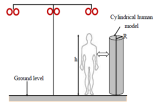
Electromagnetically, the human organism is a non-homogenous, diamagnetic, dispersive, and conductive medium. Due to the complex geometry of the human body, and for simplicity, it is preferable to consider the human model as a cylinder in low-frequency electric and magnetic fields. As a result, only a few distinctive tissues, such as brain, lungs, and liver, need to be described by the block model [27-31].
Note that the simplified physical modeling of the human body as a cylindrical representation has already been shown to be effective in the evaluation of induced currents in the human body due to exposure to electric and magnetic fields from power lines. For this reason, in this work for the case study of HV power lines, the main feature of the model is the efficiency and the rapid estimation of the phenomenon [32-35].
In general, the human body perturbs significantly in a low-frequency electric field. In most cases of human exposure, the electric field is vertical with respect to the ground. At a low frequency, the human body is a good conductor, whose surface is nearly normal to the electric field. Electrical charges can deposit on the surface of the body. Then, the electric current density J produced by the internal field may be expressed as [31]:
J=ω.σ=ω.ε0.En (19)
where, σ is the conductivity of the human body; En is the normal component of the electric field calculated at the boundary point and is equal to the calculated field at the boundary point on the human body; ω is the angular frequency of the voltage of the HV power line; is the complex penetration depth; ε0 is the permittivity of the free space.
On the other hand, human body does not perturb the magnetic field, and the magnetic field in tissue is the same as the external field, since the magnetic permeability of tissues is the same as that of air. If a magnetic induction field with a supposed uniform intensity on the surface of the ground, and is directed perpendicular to this same surface. In the simplest model of an equivalent circular loop corresponding to a given body contour, the current density can be expressed mathematically as [31]:
J=π.f.σ.R.B (20)
where, f is the frequency of power source; R is the loop radius; B is the magnetic flux density vector normal to the current loop; σis the electrical conductivity of the human body (tissue).
Figure 2 provides a simplified 2D model of the human body.
Figure 2. A simplified 2D model of the human body
2.4 Krill Herd Algorithm (KH)
Krill herd (KH) algorithm provides a novel meta-heuristic swarm intelligence optimization method. It mimics the herding of krill swarms in response to specific biological and environmental processes. In the search space, the position of an individual krill is mainly affected by three actions [36-39]: movement induced by other krill individuals, foraging, and random diffusion.
In KH algorithm, the Lagrangian model is applied within predefined search space, which is given as:
dXidt=Ni+Fi+Di (21)
where, F, N, and D are the foraging motion, the motion induced by other krill individuals and the random physical diffusion of the krill i, respectively [36-39].
In the first step, the direction of the induced movement αi is approximated by the target effect, local effect, and repulsive effect. For a krill, this movement can be expressed as:
Nnewi=Nmax (22)
where,{{N}^{\max }}, {{\omega }_{n}}andN_{i}^{old} are the maximum speed, inertia weight, and the previous movement, respectively.
In the second step, the foraging involves two elements: food location and previous experience. For the {{i}^{th}} krill, foraging can be idealized as:
{{F}_{i}}={{V}_{f}}{{\beta }_{i}}+{{\omega }_{f}}F_{i}^{old} (23)
where,
{{\beta }_{i}}=\beta _{i}^{food}+\beta _{i}^{best} (24)
where, {{V}_{f}} is the foraging speed; {{\omega }_{f}} is the inertia weight of foraging motion in (0,1); F_{i}^{old} is the last foraging motion; \beta _{i}^{food}is the attractiveness of food; \beta _{i}^{best} is the best known fitness of the {{i}^{th}} krill [36-39].
In the third step, random diffusion is computed based on a maximum diffusion speed and a random directional vector. It’s given as [36-39]:
{{D}_{i}}={{D}^{\max }}\delta (25)
where, {{D}^{\max }} is the maximum diffusion speed; \delta is the random directional vector in [−1, 1].
Through the three previously mentioned steps, the position in KH from \left( t \right) to \left( t+\Delta t \right)can be formulated as [36-39]:
{{X}_{i}}\left( t+\Delta t \right)={{X}_{i}}\left( t \right)+\Delta t\frac{d{{X}_{i}}}{dt} (26)
2.5 Grasshopper Optimization Algorithm (GOA)
The grasshopper optimization algorithm (GOA) is a novel meta-heuristic algorithm inspired by the swarm behavior of grasshoppers and their social interaction. In a swarm, the position of each grasshopper depends on three forces: social interaction, gravity, and wind advection [40-44].
The mathematical model employed to simulate the swarm behavior can be described by:
{{X}_{i}}={{S}_{i}}+{{G}_{i}}+{{A}_{i}} (27)
where, {{X}_{i}} is the position of the {{i}^{th}} grasshopper; {{S}_{i}},{{G}_{i}} and {{A}_{i}} are the social interaction, gravity, and wind advection of the {{i}^{th}} grasshopper, respectively.
The social interaction force between grasshoppers can be defined as [40-44]:
{{S}_{i}}=\sum\limits_{j=1}^{N}{s\left( {{d}_{ij}} \right)}\widehat{{{d}_{ij}}}j\ne i (28)
where, {{d}_{ij}}is the distance measured between the {{i}^{th}} and {{j}^{th}} grasshopper; s is a function of the social attraction and repulsion between grasshoppers, it can be defined as follow [40-44]:
s\left( r \right)=f{{e}^{\frac{-r}{l}}}-{{e}^{-r}} (29)
where, f and l are the intensity and length scale of the attraction, respectively.
The gravity that affects grasshopper positions can be calculated by [40-44]:
{{G}_{i}}=-g.{{\hat{e}}_{g}} (30)
where, gis the gravitational constant; {{\hat{e}}_{g}} is the unity vector of gravity.
In the nymph stage, grasshopper’s movements are related to wind direction, as they have no wings. The wind direction can be calculated by [40-44]:
{{A}_{i}}=u.{{\hat{e}}_{\omega }} (31)
where, uis a constant drift; {{\hat{e}}_{\omega }} is the unity vector of wind direction.
The position of a grasshopper can be calculated by [40-44]:
{{X}_{i}}=\sum\limits_{j=1}^{N}{s\left( \left| {{x}_{j}}-{{x}_{i}} \right| \right)}\frac{{{x}_{j}}-{{x}_{i}}}{{{d}_{ij}}}-g{{\hat{e}}_{g}}+u{{\hat{e}}_{\omega }} (32)
To prevent grasshoppers from reaching the comfort zone too quickly and enable the swarm to converge to the global optimum, the above equation can be modified as [40-44]:
{{X}_{i}}=c\sum\limits_{j=1}^{N}{c\left( \frac{u{{b}_{d}}-l{{b}_{d}}}{2}s \right.\left( \left| x_{j}^{d}-x_{i}^{d} \right| \right)}\frac{{{x}_{j}}-{{x}_{i}}}{{{d}_{ij}}}+{{\overset{\scriptscriptstyle\frown}{T}}_{d}} (33)
where, u{{b}_{d}}and l{{b}_{d}}are the upper and lower bounds in the {{d}^{th}}dimension, respectively; {{\overset{\scriptscriptstyle\frown}{T}}_{d}}is the target value in the {{d}^{th}} dimension.
To reduce the comfort zone, repulsion zone, and the attraction zone, an attenuation coefficient can be defined as [40-44]:
c={{c}_{\max }}-l\frac{{{c}_{\max }}-{{c}_{\min }}}{L} (34)
where, {{c}_{\max }} and {{c}_{\min }} are the maximum and minimum values, respectively; l is the current iteration; L is the maximum number of iterations.
In the Charge Simulation Method (CSM), the objective function used for optimization (minimization) can be given by [17]:
OF=\frac{1}{{{n}_{t}}}\left| \sum\limits_{i=1}^{{{n}_{c}}}{\frac{{{V}_{{{c}_{i}}}}-{{V}_{{{v}_{i}}}}}{{{V}_{{{c}_{i}}}}}} \right|100 (35)
where, {{V}_{{{c}_{i}}}} is the potential applied to phase conductors; {{V}_{{{v}_{i}}}} is the potential obtained by the check charges; {{n}_{t}} is the total number of check points.
For the Current Simulation Technique (CST), the objective function can be described by [23]:
OF=\frac{1}{{{n}_{t}}}\sum\limits_{i=1}^{{{n}_{c}}}{\left| \frac{{{A}_{{{c}_{i}}}}-{{A}_{{{m}_{i}}}}}{{{A}_{{{c}_{i}}}}} \right|}100 (36)
where, {{A}_{{{c}_{i}}}} is the magnetic potential calculated by the current points; {{A}_{{{m}_{i}}}} is the new magnetic potential estimated by the matching points; {{n}_{c}} is the total number of matching points.
The objective of this optimization carried out by these objective functions is to ensure a very precise calculation of the electric field and of the magnetic induction.
2.6 Finite Element Method (FEM)
As a numerical technique, the Finite Element Method (FEM) provides an efficient and mathematically satisfying way to approximate the solution of partial differential equations. By this approach, a given differential or integral equation can be approximated in four steps [45-49]:
Step 1: Discretize the solution space into a finite number of sub-spaces or elements;
Step 2: Derivation of governing equations for a typical element;
Step 3: Gather all the elements in the solution space;
Step 4: Solving the set of obtained equations.
In quasi static analysis, the magnitudes of the electric field E and magnetic induction B are derived from the gradient of the potential V and from the magnetic vector potential A, as shown below, respectively [48, 49].
\overset{\to }{\mathop{\text{E}}}\,=-\overrightarrow{grad}.V (37)
\overset{\to }{\mathop{B}}\,=\overrightarrow{rot}.\overset{\to }{\mathop{A}}\, (38)
The numerical simulation is performed by the software of COMSOL Multiphysics (version 4.3b) in 2D geometry. An Electrostatic and Magnetostatic modules of COMSOL have been used to determine the values of the electric field and magnetic induction by solving completely the Poisson’s equations [50].
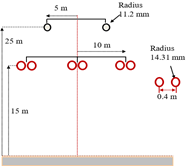
Figure 3. 400 kV single circuit three-phase overhead power line
This case study targets a three-phase HV power line of 400 kV, with two ground wires. The arrangement and geometric coordinates are shown in Figure 3. It is assumed that the three-phase currents flow in a balanced process with a size of 1000 A, with a nominal frequency of 50 Hz. The ground is assumed to be homogeneous with a resistivity of 100 Ω.m.
Before accessing to the computation of the electric field and magnetic induction, it is necessary to optimize the number and position of the simulation charges and the current loops in the sub-conductors, using hybrid techniques combining the proposed methods with the evolutionary algorithms mentioned previously above.
To ensure a fair comparison, the experiments for each algorithm were repeated 15 times, and the best parameter values according to objective functions were selected.
The parameter settings of the optimization algorithms adopted in this study are presented in Table 1.
Table 1. Parameter settings of KH and GOA algorithms
|
Algorithms |
Parameters setting |
|
KH |
Iteration Max=100 Max induced speed Nmax=0.01 (inms-1) Foraging speed Vf =0.02 (inms-1) Max diffusion speed Dmax = 0.005(inms-1) |
|
GOA |
Iteration Max=100 Search agents=20 cmax=1; cmin=0.00001. |
Figure 4. Variation of objective functions with the number of iterations for the charge simulation method (CSM)
Figures 4 and 5 show the convergence of the objective functions defined by equations (35 and 36) with the number of iterations. It can be seen that the values of the objective functions decrease with the increasing number of iterations, because they converge towards the optimal solution.
As shown in Figures 4 and 5, the KH algorithm has achieved a more minimum value of the objective function than the GOA algorithm, which indicates that the KH algorithm works better and more efficient in solving this minimization problem than the GOA algorithm.
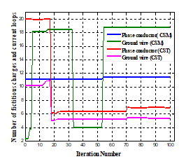
The simulation results obtained by the KH algorithm for different best parameter values to be used in the proposed techniques are presented in Figures 6 and 7, where it becomes clear that the KH algorithm converges quickly to these optimum values.
Figure 5. Variation of objective function with the number of iterations for the current simulation technique (CST)
Figure 6. Convergence of the number of fictitious charges with current loops
Figure 7. Convergence of the position of fictitious charges with current loops
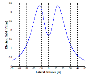
Figure 8 shows the lateral distribution of electric field intensity at different points 1m above the ground. The electric field reached the maximum intensity under the side phase conductors, and the minimum intensity at the middle phase conductor, for the phase shift of the line voltages cancels out the generated field. It is also clear that the electric field decreased gradually with the lateral distance to the center of the power line. The maximum peak intensity of the electric field did not exceed the public exposure level of 5 kV/m specified in the ICNIRP guidelines.
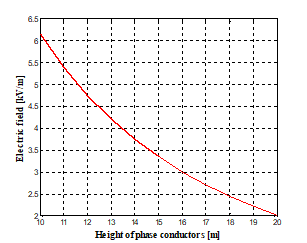
Figure 9 illustrates the effect of varying the height of the phase conductors above ground level. This variation changes the capacitance of the power line to earth, which varies the net charges density to maintain its potential. Since the capacitance decreases with increasing height, a reduction in electric field intensity is expected at (1 m) above ground level. Therefore, an increase in the height of the conductors above the ground leads to a significant reduction in the electric field value.
Figure 8. Eletric field profile at 1m above the ground obtained by the Hybrid Method (CSM+KH)
Figure 9. Effect of phase conductors’ height above ground on electric field intensity
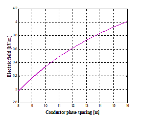
The effect of varying the spacing between the phase conductors on electric field intensity is illustrated in Figure 10. An increase in this spacing causes an increase in the electric field intensity above the ground.
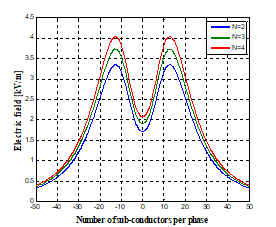
Figure 11 shows the effect of bundle phase conductors on the electric field intensity, as seen in this figure, the electric field is greatly increased if the number of sub-conductors per phase is increased.
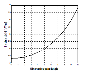
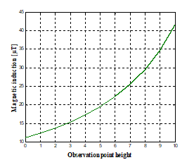
The electric field intensity at different heights of observation point above ground was calculated, as shown in Figure 12. It is clear that the electric field intensity increases as the observation point height above ground increases.
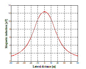
Figure 13 illustrates the lateral distribution of the magnetic induction at 1 m above the ground. It can be seen that the magnetic induction reached the peak under the middle phase conductor, and weakened with the growing lateral distance from the center of the power line. The peak of the magnetic induction was well below the safe limit of 200 μT for public exposure, as mentioned in the ICNIRP guidelines.
Figure 10. Effect of spacing between phase conductors on electric field intensity
Figure 11. Effect of the number of sub-conductors per phase on electric field intensity
Figure 12. Effect of the height of observation point above the ground on electric field intensity
Figure 13. Magnetic induction profile at 1m above the ground obtained by the Hybrid Method (CST+KH)
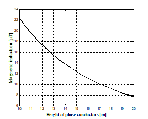
Figure 14. Effect of phase conductors’ height above ground on magnetic induction intensity
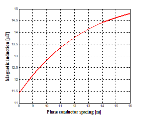
Figure 15. Effect of spacing between phase conductors magnetic induction intensity
Similar to the electric field, the intensity of the magnetic induction is also dependent on the factors mentioned above. As shown in Figures 14, 15 and 16, an increase in height phase’s conductors above the ground level decreases rapidly the magnetic induction intensity.The increase in spacing between the phase conductors increases the magnetic induction intensity. The magnetic induction intensity increases as the observation point height above ground increases.
Figure 16. Effect of the height of observation point above the ground on magnetic induction
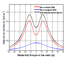
Figure 17. Distribution of the induced current density in human body
Figure 18. Meshing of the computational domain
Figure 17 shows the induced current density in a human body (head radius: 0.15 m; body conductivity: 0.2 S/m) at different distances from the center of the HV power line. The induced current was very sparse under the middle phase conductor. As the position moved away from that conductor, the induced current density gradually increased to the peak at a particular distance. From the peak position, the induced current density started to decline quickly, as the distance increased from the center of the power line. The maximum density of the induced current was below the safe level specified in the ICNIRP guidelines.
To verify the results accuracy of the proposed hybrid approaches, the electrostatic and magnetostatic modules of COMSOL Multiphysics 4.3b in 2D space are recommended, this software adopts the finite element method (FEM) to simulate the electric field and magnetic induction of the HV power line. The computational domain illustrated in Figure 2 above was meshed into linear triangular elements by the COMSOL Multiphysics 4.3b software, as shown in Figure 18.
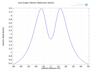
Figure 19. Electric field profile at 1 m above the ground obtained by COMSOL Multiphysics 4.3b
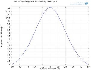
Figure 20. Magnetic induction profile at 1 m above the ground obtained by COMSOL Multiphysics 4.3b
The comparison of the profiles of the electric field and of the magnetic induction carried out by the finite element method under COMSOL Multiphysics 4.3b is presented in Figures 19 and 20.
As shown in Figure 19, a lower value of electric field intensity appeared under the center of the HV power line. From that position, the electric field intensity started to increase to the peak value nearly under the lateral conductors, beyond that, the electric field decreases rapidly with the lateral distance from the HV power line center. However, as illustrated in Figure 20, the magnetic induction reached the peak value under the middle phase conductor, from where it began to decline gradually with the growing lateral distance from the HV power line center.
Figures 21 and 22 compare the results obtained by the adopted hybrid approaches with those simulated by COMSOL Multiphysics 4.3b. As noted, the various results are in reasonably good agreement, which demonstrates the accuracy and the performance of the proposed approachs.
Finally, in order to confirm the validity of the proposed hybrid methods, the simulation results were compared with the measurements data taken during an experimental work available in the literature [12] for the same geometry of the power line configuration.
Figure 21. Electric field intensities obtained by the (CSM+KH) method and COMSOL Multiphysics 4.3b
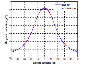
Figure 22. Magnetic induction intensities obtained by the (CST+KH) method and COMSOL Multiphysics 4.3b
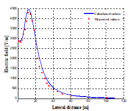
Figure 23. Comparison between measured and calculated lateral profiles of electric field intensity
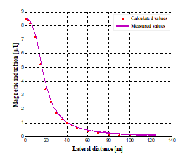
Figure 24. Comparison between measured and calculated lateral profiles of magnetic induction intensity
Figures 23 and 24 show both the measured and computed results. As it can be seen, a satisfactory agreement between the computational results and measurements is obtained. The maximum error value is not significant; it does not exceed the value of 5%. it can be also clearly observed from this comparison that the measured values of the electric and magnetic fields are relatively lower than the calculated values mainly because of the objects encountered which act as screens and the ground conditions which are often very far from the ideal conditions taken in the simulation since the ground is not flat and there is vegetation and the conductors of the line are not horizontal of infinite length and are not parallel to the ground.
This article presents a rigorous modeling coupling a new methodology of simulation with optimization algorithms for evaluating the electric field and magnetic induction under a 400 kV overhead power line. The objective of optimization algorithms consists of determining the position and number of fictitious charges and filament current loops which are necessary for a very precise calculation. From the results, the KH algorithm has proven to have excellent performance compared with GOA Optimization algorithm. The results show that the electric field intensity is most intense nearly under the side phase conductors, and less intense under the middle phase conductor. The intensity of the electric field decreases quickly with the lateral distance from the HV power line center. Regarding the magnetic induction distribution, the peak value is marked below the middle phase conductor, and then decreases with increase in lateral distance from the HV power line center. It was also found that both the electric field and magnetic induction depend on many factors. The maximum obtained values of electric field and the magnetic induction at 1 m above the ground are well less than the acceptable limits set by the international ICNIRP standard. The results obtained by the adopted methods were compared with those gained from the COMSOL Multiphysics 4.3b for the same HV power line configuration; a very better similarity of performance is observed. In addition, these results were also verified using the measured values available in the literature, a good agreement is observed. As a result, this comparison is completely satisfactory and may well confirm the validation of the adopted hybrid approaches.
[1] Cigré. (1980). Electric and Magnetic Field Produced by Transmission Systems, Working Group 01 (Interference and Fields) of Study Committee 36, Paris. https://e-cigre.org/publication/21-electric-and-magnetic-fields-produced-by-transmission-systems.
[2] Dib, D, Mordjaoui, M. (2014). Study of the influence high-voltage power lines on environment and human health (case study: The electromagnetic pollution in Tebessa city, Algeria). Journal of Electrical and Electronic Engineering, 2(1): 1-8. https://doi.org/10.11648/j.jeee.20140201.11
[3] Nwoke, J.E., Onimisi, M.Y., Jonah, S.A., Tafida, R.A. (2017). Measurement and analysis of health effects due to exposure to non-ionizing radiation from high tension cables around Kaduna Metropolis, North West, Nigeria. American Journal of Condensed Matter Physic, 7(3): 73-80. https://doi.org/10.5923/j.ajcmp.20170703.03
[4] Kulkarni, G., Gandhare, W.Z. (2012). Proximity effects of high voltage transmission lines on humans. Int. J. on Electrical and Power Engineering, 3(1): 1-11.
[5] Review of the scientific evidence for limiting exposure to electromagnetic fields (0–300 GHz), Doc. NRPB, vol. 15, no. 3, National Radiological Protection Board, 2004.
[6] IEEE Standard for Safety Levels with Respect to Human Exposure to Electromagnetic Fields, 0-3 kHz. IEEE Std C95.6-2002, Oct. 2002.
[7] Nicolaou, C.P., Papadakis, A.P., Razis, P.A., Kyriacou G.A., Sahalos, J.N. (2011). Measurements and predictions of electric and magnetic fields from power lines. Electric Power Systems Research, 81(5): 1107-1116. https://doi.org/10.1016/j.epsr.2010.12.014
[8] Ayad A.N.E.I., Krika W., Boudjella H., Benhamida F., Horch A. (2019). Simulation of the electromagnetic field in the vicinity of the overhead power transmission line, European Journal of Electrical Engineering, 21(1): 49-53. https://doi.org/10.18280/ejee.210108
[9] Ali, Y.S.M., El-Baset, A.A., Elghaffar, A.N.A. (2016). Mathematical calculation of electromagnetic field in high voltage substation to treatment its effect on the protective equipements. Annals of Faculty Engineering Hunedoara - International Journal of Engineering, 14(4): 139-146.
[10] Unde, M., Maske, R., Kushare, B. (2013). Safety evaluation of live line operators of 1200 KV UHV AC exposed to electric and magnetic fields. ACEEE International Journal on Electrical and Power Engineering, 4(3): 26-32.
[11] ICNIRP, International Commission on Non-Ionizing Radiation Protection. (2010). Guidelines for limiting exposure to time-varying electric and magnetic fields (1Hz to 100 kHz), Health Physics, 99(6): 818-836. https://doi.org/10.1097/HP.0b013e3181f06c86
[12] Vujević, S., Lovrić, D., Modrić, T. (2011). 2D computation and measurement of electric and magnetic fields of overhead electric power lines. Proceedings of the Joint INDS'11 & ISTET'11, International Workshop on Nonlinear Dynamics and Synchronization (INDS) and International Symposium on Theoretical Electrical Engineering (ISTET), pp. 1-6. https://doi.org/10.1109/INDS.2011.6024796
[13] Kato, Y. (1980). A Charge Simulation Method for the Calculation of Two Dimensional Electrostatic Fields. Memoirs of the Fukui Institute of Technology, 10: 107-117.
[14] Singer, H., Steinbigler, H., Weiss, P. (1974). A charge simulation method for the calculation of high voltage fields. IEEE Transactions on Ower Apparatus and Systems, PAS-93(5): 1660-1668. https://doi.org/10.1109/TPAS.1974.293898
[15] Malik, N.H. (1989).A review of the charge simulation method and its applications. IEEE Transactions on Electrical Insulation, 24(1): 3-20. https://doi.org/10.1109/14.19861
[16] Djekidel, R., Choucha, A., Hadjaj, A. (2017). Efficiency of some optimisation approaches with the charge simulation method for calculating the electric field under extra high voltage power lines. IET Generation, Transmission & Distribution, 11(17): 4167-4174. https://doi.org/10.1049/iet-gtd.2016.1297
[17] Djekidel, R., Bessedik, S.A., Hadjadj, A. (2018). Electric field modeling and analysis of EHV power line using improved calculation method. Facta universitatis-series: Electronics and Energetics, 31(3): 425-445. https://doi.org/10.2298/FUEE1803425D
[18] Djekidel, R., Bessedik, S.A., Akef, S. (2020). 3D Modelling and simulation analysis of electric field under HV overhead line using improved optimisation method. ET Science, Measurement & Technology, 14(8): 914-923. https://doi.org/10.1049/iet-smt.2019.0137
[19] Lubin, T., Mezani, S., Rezzoug, A. (2012). 2D analytical calculation of magnetic field and electromagnetic torque for surface-inset permanent magnet motors, IEEE Transactions on Magnetics, Institute of Electrical and Electronics Engineers. https://doi.org/10.1109/TMAG.2011.218091
[20] Abdel-Salam, M., Abdallah, H., El-Mohandes, M.T., El-Kishky, H. (1999). Calculation of magnetic fields from electric power transmission lines. Electric Power Systems Research, 49(2): 99-105. https://doi.org/10.1016/S0378-7796(98)00078-9
[21] Yao, D.G., Li, B., Deng, J., Huang, D.M., Wu, X.H. (2008). Power frequency magnetic field of heavy current transmit electricity lines based on simulation current method. IEEE World Automation Congress, pp. 1-4.
[22] Roshdy, R., Mazen, A.S., Abdel-Bary, M., Mohamed, S. (2011). Laboratory validation of calculations of magnetic field mitigation underneath transmission lines using passive and active shield wires. Innovative Systems Design and Engineering, (4): 218-232.
[23] Djekidel, R., Bessedik, S.A., Akef, S. (2019). Accurate computation of magnetic induction generated by HV overhead power lines, Facta Universitatis, Series: Electronics and Energetics, 32(2): 267-285. https://doi.org/10.2298/FUEE1902267R
[24] Sunderland, K., Coppo, M., Conlon, M., Turri, R. (2016). A correction current injection method for power flow analysis of unbalanced multiple-grounded 4-wire distribution networks. Electric Power Systems Research, 132: 30-38. https://doi.org/10.1016/j.epsr.2015.10.027
[25] Albano, M., Turri, R., Dessanti, S., Haddad, A., Griffiths, H., Howat, B. (2006). Computation of the electromagnetic coupling of parallel untransposed power lines. Proceedings of the 41st International Universities Power Engineering Conference, pp. 303-307. https://doi.org/10.1109/UPEC.2006.367764
[26] Djekidel, R., Bessedik, S.A., Spitéri, P., Mahi, D. (2018). Passive mitigation for magnetic coupling between HV power line and aerial pipeline using PSO algorithms optimization. Electric Power Systems Research, 165: 18-26. https://doi.org/10.1016/j.epsr.2018.08.014
[27] Yildirim, H., Kalenderli, O. (2003). Computation of electric field induced currents on biological bodies near high voltage transmission lines. 13th International Symposium on High Voltage Engineering, Delft, Netherlands, pp. 1-4.
[28] El-Makkawy, S.M. (2007). Numerical determination of electric field induced currents on human body standing under a high voltage transmission line. 2007 Annual Report - Conference on Electrical Insulation and Dielectric Phenomena, pp. 802-806. https://doi.org/10.1109/CEIDP.2007.4451651
[29] Češelkoska, V.C. (2004). Interaction between LF electric fields and biological bodies. Serbian Journal of Electrical Engineering, 1(2): 153-166.
[30] Kulkarni, G., Gandhare, W.Z. (2012). Proximity effects of high voltage transmission lines on humans. International Journal on Electrical and Power Engineering, 3(1): 28-32.
[31] Ozovehe, A., Ibrahim, M., Hamdallah, A. (2012). Analysis of electromagnetic pollution due to high voltage transmission lines. Journal of Energy Technologies and Policy, 2(7): 1-10.
[32] Abdel-Salam, M., Abdallah, M. (1995). Transmission-line electric field induction in humans using charge simulation method. IEEE Trans. Biomed. Eng., 42(11): 1105-1109.
[33] Talaat, M. (2010). Charge simulation modeling for calculation of electrically induced human body currents. IEEE Annual Report Conference on Electrical Insulation and Dielectric Phenomena CEIDP, pp. 1-4. https://doi.org/10.1109/CEIDP.2010.5723972
[34] Barchanski, A., Clemens, M., De Gersem, H., Weiland, T. (2006). Efficient calculationof current densities in the human body induced by arbitrarily shaped, low-frequency magnetic field sources. J. Comput. Phys., 214: 81-95.
[35] Talaat, M. (2014). Calculation of electrostatically induced field in humans subjected to high voltage transmission lines. Electric Power Systems Research, 108: 124-133. https://doi.org/10.1016/j.epsr.2013.11.004
[36] Gandomi, A.H., Alavi, A.H. (2012). Krill herd: A new bio-inspired optimization algorithm. Communications in Nonlinear Science and Numerical Simulation, 17(12): 4831-4845. https://doi.org/10.1016/j.cnsns.2012.05.010
[37] Wang, G., Guo, L.H., Gandomi, A.H., Cao, L.H., Alavi, A.H., Duan, H., Li, J. (2013). Lévy-flight krill herd algorithm. Mathematical Problems in Engineering, 2013: 682073. https://doi.org/10.1155/2013/682073
[38] Wang, G.G., Gandomi, A.H., Alavi, A.H. (2014). An effective krill herd algorithm with migration operator in biogeography-based optimization. Applied Mathematical Modelling, 38(s9-10): 2454-2462. https://doi.org/10.1016/j.apm.2013.10.052
[39] Wang, G.G., Guo, L.H., Gandomi, A.H., Alavi, A.H., Duan, H. (2013). Simulated annealing-based krill herd algorithm for global optimization. Advances in Nonlinear Analysis and Optimization, 2013: 213853. https://doi.org/10.1155/2013/213853
[40] Saremi, S., Mirjalili, S., Lewis, A. (2017). Grasshopper optimisation algorithm: Theory and application. Advances in Engineering Software, 105: 30-47. https://doi.org/10.1016/j.advengsoft.2017.01.004
[41] Luo, J., Chen, H., Zhang, Q., Xu, Y., Huang, H., Zhao, X.A. (2018). An improved grasshopper optimization algorithm with application to financial stress prediction. Applied Mathematical Modelling, 64: 654-668. https://doi.org/10.1016/j.apm.2018.07.044
[42] Mafarja, M., Aljarah, I., Faris, H., Hammouri, A.I., Al-Zoubi, A.M., Mirjalili, S. (2019). Binary grasshopper optimisation algorithm approaches for feature selection problems. Expert Systems with Applications, 117: 267-286. https://doi.org/10.1016/j.eswa.2018.09.015
[43] Mafarja, M., Aljarah, I., Heidari, A.A., Hammouri, A.I., Faris, H., Al-Zoubi, A.M., Mirjalili, S. (2017). Evolutionary population dynamics and grasshopper optimization approaches for feature selection problems. Knowledge-Based Systems, 145: 25-45. https://doi.org/10.1016/j.knosys.2017.12.037
[44] Zhao, R., Ni, H., Feng, H.W., Song, Y.Q., Zhu, X.Y. (2019). An improved grasshopper optimization algorithm for task scheduling problems. International Journal of Innovative Computing, Information and Control, 15(5): 1967-1987.
[45] Virjoghe, E.O., Nescu, D.E., Stan, M.F., Cobianu, C. (2012). Numerical determination of electric field around a high voltage electrical overhead line. Journal of Science and Arts, 4(21): 487-496.
[46] Haldar, M.K. (2006). Introducing the finite element method in electromagnetics to undergraduates using Matlab. International Journal of Electrical Engineering Education, 43(3): 232-244. https://doi.org/10.7227/IJEEE.43.3.4
[47] Lu C., Shanker, B. (2005). Solving boundary value problems using the generalized (partition of unity) finite element method. IEEE Conference on Antennas and Propagation Society International Symposium, 1B: 125-128. https://doi.org/10.1109/APS.2005.1551500
[48] Sadiku, M.N.O. (2000). Numerical Techniques in Electromagnetics, 2nd edition. Boca Raton, CRC Press.
[49] Young, W.K., Hyochoong, B. (2000). The Finite Element Method Using MATLAB, London, CRC Press, Taylor & Francis Group.
[50] Ali Rachedi, B., Babouri, A., Berrouk, F. (2014). A study of electromagnetic field generated by high voltage lines using COMSOL Multiphysics. IEEE International Conference on Electrical Sciences and Technologies in Maghreb, pp. 1-5. https://doi.org/10.1109/CISTEM.2014.7076989