Samira Boumous | Nacereddine Guettaf | Amina Hamel | Ilham Lariche | Hamou Nouri*
© 2021 IIETA. This article is published by IIETA and is licensed under the CC BY 4.0 license (http://creativecommons.org/licenses/by/4.0/).
OPEN ACCESS
The quality of electrical energy and the fight against energy losses are a crucial issue for electricity companies. The use of high voltage lines can limit energy losses for the transmission of electricity over long distances. But this solution has the disadvantage of the propagation of the electromagnetic wave which has a great influence on human health. The work presented in this study mainly deals with modelling problems that may be encountered by the community working in the field of low frequency electromagnetic fields. In order to model a power line, we are based on geometric data as well as phase and earth conductor data.
electrical networks, magnetic field, transmission line characteristics, high voltage, mathematical modelling, numerical simulation, health
The electric power transmitted on an overhead line increases approximately with the surge impedance loading or the square of the system’s operating voltage. The rapidly increasing transmission voltage level in recent decades is a result of the growing demand for electrical energy. However, environmental concerns have imposed limitations on system expansion resulting in the need to better utilize existing transmission systems.
High voltages are even more extensively used in applied physics (accelerators, electron microscopy, etc.), electro-medical equipment (X-rays), industrial applications (precipitation and filtering of exhaust gases in thermal power stations and the cement industry; electrostatic painting and powder coating, etc.), or communications electronics (TV, broadcasting stations). Therefore, the requirements on voltage shape, voltage level, and current rating, short- or long-term stability for every HVDC generating system may differ strongly from each other. With the knowledge of the fundamental generating principles, it will be possible, however, to select proper circuits for a special application. The most important applications of high voltage technology are in the field of equipment and systems for the transmission and distribution of electrical energy [1-3].
A pair of overhead transmission lines generates magnetic field intensity in space. A growing concern in society is the effect these magnetic (and electric) fields have on living organisms. In particular, some studies have implicated high magnetic fields due to overhead transmission lines with higher-than-average cancer rates for those exposed. Most of these studies suggest, without being conclusive, that low-frequency fields, such as those produced by AC distribution lines, are at fault. As power requirements grow, there is an increasing need to use higher voltages on transmission lines. Power distributions above 1 MV already exist. What are the magnetic field intensities we can expect at ground levels? Typically, the distance between lines is a few meters to prevent the lines from touching during storms, and the lines may be as high as 20-25 m. This produces magnetic field intensities at ground level that may exceed 5 A/m.
The first effect to notice is that there is a force between the two magnets. The magnets either attract or repel each other. Since attraction happens at a distance, each magnet must have a domain in which it attracts the other magnet. This is exactly what we called a field. That the field is a vector field we can establish using a compass as a measuring device. The direction of the force is established by the direction of the compass needle in space. Placing the compass at as many positions as we wish, a complete map of the vector field is established. This simple measurement establishes the following [4]:
(1) A field exists throughout space.
(2) The field is stronger and closer to the magnet.
(3) The two ends of the magnet behave differently; one attracts the north pole of the compass and is labelled the South Pole; the other attracts the south pole of the compass and is labeled the north pole of the magnet. This arbitrary identification is convenient because of its relation with the Earth’s magnetic field.
(4) By placing the compass at different locations in space, we can map the magnetic field.
Therefore, calculation of the magnetic field distribution underneath overhead transmission lines is of great importance and should be elaborated. The magnetic field impact on environment and interaction with human beings are also of great interest.
Consequently, a precise calculation of the magnetic field underneath overhead transmission lines is an important task in transmission line design. Quantitative description of the magnetic field around overhead transmission lines has been presented in many papers [3-5] The magnetic field effect on transmission lines maintenance crew is an important issue that the electric utilities are most often required paying attention to the potential health hazards [4].
Since the early 1970s, the risks of electromagnetic fields associated with 50 Hz (60 Hz) generated by high voltage lines have been widely addressed by the scientific community to the World Health Organization [5-12].
The objective of this work is to reduce the impact of high voltage lines on health. We try to protect our health against the undesirable effects of the electromagnetic field induced by very high voltage lines. In addition, this type of energy transport creates problems that require the installation of huge compensation devices to ensure the stability of the electricity grid.
So, our contribution is to quantify the exposure to currents of power transmission lines of the population far and near high voltage power lines. It was necessary to research and demonstrate the impact of high tensions on the human body.
2.1 The geometric model used
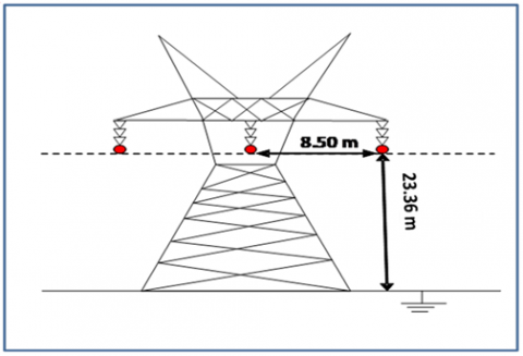
The real model of the high voltage line is shown in Figure 1. The dimensions of the real model data are very useful for numerical simulation. We note that whatever the model used in electromagnetic, depends on the geometric parameters of the system.
Figure 1. Real model of the 400 KV line
The simplified model of the system to be studied is represented in Figure 2. It is a partial representation of an existing system in order to test and validate certain aspects and / or the functional behaviour or simply informative of an implementation or of a project:
Representation can be real at a given scale;
The representation can be virtual: digital graphic model in two dimensions or in perspective.
Figure 2. The model simplifies of 400 kV high voltage line
2.2 Usual data used in simulation
Number of phases: 3;
Number of conductors for each phase: 2;
Transmitted power: Pn = 1200 MW;
Resistance r = 0.08 W/km;
Inductance: L = 0.4 mH/km;
Capacitance: C = 10 F/km;
Nominal current: In = 322 A;
Maximum voltage of each phase: Umax = 400 kV;
Maximum current for each phase and for each conductor: Imax = 1 kA;
Properties of the conductor used:
Maximum length of conductors in each phase: Ll = 350 km;
Type: ACSR _ Aluminum Conductor, Steel Reinforced
Section: S = 350 mm²;
Volumic mass: r= 2.6 kg/dm3;
Electrical resistivity: ral = 36,232 W.mm2/km for 90℃;
Thermal conductivity: l= 204 W/(m.K);
Specific heat capacity: Cth = 0,879 kJ/(kg.K);
Coefficient of expansion: a = 23,8.10-6 K-1;
Melting temperature: Tf = 658℃.
2.3 Magnetic field in the vicinity of the ground for a single conductor
Ampere’s Law is similar to Gauss’ Law, as it allows us to determine the magnetic field that is produced by an electric current in configurations that have a high degree of symmetry. The first fundamental law of magneto statics gives us according to the Ampere’s Law [13, 14]:
$\oint_{C} \overrightarrow{H .\overrightarrow{d l}}=I_{e n c}.$ (1)
where, the integral on the left is a “path integral”, similar to how we calculate the work done by a force over a particular path (Figure 3). The circle sign on the integral means that this is an integral over a “closed” path; a path where the starting and ending points are the same. Ienc is the net current that crosses the surface that is defined by the closed path, often called the “current enclosed” by the path, H is the magnetic field and dl the elementary element of length L.
We will apply the Ampere’s Law in the case of the long and rectilinear wire traversed by a given current I. Consider a contour circle (c), in a plane perpendicular to the axis of the conductor, centered on this one (Figure 3).
Figure 3. Circulation of a magnetic field along a closed curve
For reasons of symmetry, the magnetic field H is constant throughout the circle. If the radius of the latter is r, the magnetic field will be given by:
$H=\frac{I}{2 \pi r}$ (2)
The magnetic induction is given by:
$\vec{B}=\mu \vec{H}$ (3)
where, μ is the magnetic permeability.
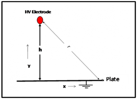
For our case and for any triangle (Figure 4), we can write the distribution in terms of magnetic field as a function only of the variables x and y [15]:
$\vec{B}=\frac{\mu_{0} \vec{I}}{2 . \pi \cdot r}=\frac{\mu_{0} \cdot \vec{I}}{2 \pi \sqrt{h^{2}+x^{2}}}$ (4)
Figure 4. Configuration of a single conductor
2.3 Magnetic field for a single conductor
The magnetic field varies with the current flowing in the line. It is also a function of the geometry of the conductors and the current flowing in all the nearby conductors. The alignment of these generates a stronger magnetic field than triangle/clover geometry [16]. We consider a three-phase high-voltage overhead power line having the arrangement and geometric coordinates, related to the suspension pylon whose phase position is in a conductor layer (Figure 5).
Figure 5. Diagram used to calculate the magnetic field of a three-phase for 400 KV
We try to determine the distribution of the magnetic field (or magnetic induction) in the vicinity of the ground. The magnetic induction created by the three phases is written according to the Biot – Savart law:
$\vec{B}_{T}=\frac{\mu_{0}}{2 \pi}\left[\frac{\mathrm{I}_{\mathrm{A}}}{\mathrm{r}_{\mathrm{A}}} \overrightarrow{a_{r_{A}}}+\frac{\mathrm{I}_{\mathrm{B}}}{\mathrm{r}_{\mathrm{B}}} \overrightarrow{a_{r_{B}}}+\frac{\mathrm{I}_{\mathrm{C}}}{\mathrm{r}_{\mathrm{C}}} \overrightarrow{a_{r_{C}}}\right]$ (5)
where,
$r_{A}=\sqrt{\left(x-x_{A}\right)^{2}+\left(y-y_{A}\right)^{2}}$ (6)
$r_{B}=\sqrt{\left(x-x_{B}\right)^{2}+\left(y-y_{B}\right)^{2}}$ (7)
$r_{C}=\sqrt{\left(x-x_{C}\right)^{2}+\left(y-y_{C}\right)^{2}}$ (8)
For complex values of currents and magnetic fields, we can write the magnetic induction for three phases in the following form:
$\bar{B}_{i}=\frac{\mu_{0} . \overline{I_{i}}}{2 \pi r_{i}}$ (9)
The vertical and horizontal components for each phase of the magnetic induction field are then expressed by the following relationships:
$\left\{\begin{array}{c}B_{x i}=B_{i} \cos \left(\alpha_{i}\right) \\ B_{y i}=B_{i} \sin \left(\alpha_{i}\right)\end{array}\right.$ (10)
where, a1, a2, a3 represent the angles that form the conductors with the axis of the pylon.
The vertical and horizontal components for the 3 phases of the magnetic induction field are then expressed by the following relationships:
$\left\{\begin{array}{l}B_{x}=\sum B_{x_{i}} \\ B_{y}=\sum B_{y_{i}}\end{array}\right.$ (11)
The value of the total vector-field is given by the following relation:
$B_{T}=\sqrt{B_{x}^{2}+B_{y}^{2}}$ (12)
2.4 Magnetic induction for a three-phase system
The geometric criteria imposed by the nature of the site are very important for the design of overhead power lines, as they relate to the safety of humans and the proper functioning of the equipment [16, 17]. The variation of the conductor / earth distance leads to the variation of the magnetic field between the pylons (Figure 6).
The calculation of the mechanical stresses (spans, maximum deflection, height of the conductor, etc.) of the line depends on several factors, climatic and atmospheric. The vertical distance between the curve and the chord is called arrow.
Figure 6. Example used for the calculation the critical magnetic field (h = 15 m)
The y-coordinate of the conductor curve presents the conductor height related to the x-axis, but its x-coordinate presents a horizontal distance from the left-hand side support.
In addition, this approach will help to recognize some mathematical similarities and differences easily between the catenary and parabola.
There is a basic condition in connection with the definition of the catenary, which says that constant should be positive (C> 0).
The catenary curve yc shown in Figure 6, has the following equation [18]:
$\left.y^{*}=\operatorname{C.ch}(x / C) ; x \in\right]-\infty,+\infty[$ (13)
Conductor attached on two sides, in this case on transmission towers, will form curve in shape of a catenary. It can be considered as symmetric, if conductors are at their ends in the same height above a flat surface [19].
The transit of electricity through lines is always accompanied by the presence of:
(1) An electric field which is linked to:
The voltage.
Proximity to other phases, earth cables, earth or any nearby object.
Line configuration (90 kV, 225 kV, 400 kV, 750 kV, …).
(2) A magnetic field which is related to:
The value of the current flowing in the conductors.
Line configuration.
For this work, we will concede the balanced three-phase system. Calculation using symmetrical components is particularly useful when a three-phase network is unbalanced. The system is said to be balanced when: V1=V2=V3=V.
A three-phase voltage system is a set of three alternating voltages, of the same effective value, offset from one another by 120°:
$\left\{\begin{array}{l}v_{1}(t)=V e f f . \sqrt{2} . \cos (\omega t) \\ v_{2}(t)=V e f f . \sqrt{2} . \cos \left(\omega t-\frac{2 \pi}{3}\right) \\ v_{3}(t)=V \text { eff } \sqrt{2} \cos \left(\omega t-\frac{4 \pi}{3}\right)\end{array}\right.$ (14)
The voltage variations for the three phases are shown in the following Figure 7:
The precise knowledge of the transit intensity eliminates the need to systematically measure the magnetic field in many places, since the calculation gives fairly precise results of the magnetic field as a function of distance. It is possible to represent the currents in the following form (The three-phase equilibrium current system):
$\left\{\begin{array}{l}i_{A}=I_{m} \sin \omega t \\ i_{B}=I_{m} \sin \left(\omega t-120^{\circ}\right) \\ i_{C}=I_{m} \sin \left(\omega t+120^{\circ}\right)\end{array}\right.$ (15)
The variations of the currents for the three phases are shown in Figure 8. Note that our system is balanced.
Figure 7. Voltage variation as a function of time
Figure 8. Current variation as a function of time
To determine the variations in voltage and current along the transmission line, we use the solution of the partial differential equations system which defines the regime of the line as a function of its linear constants [20]:
$\left\{\begin{array}{l}{\left[\frac{\partial\underline V}{\partial x}\right]=[\underline{Z}].[\underline{I}]} \\ {\left[\frac{\partial \underline{I}}{\partial x}\right]=[\underline{Y}] .[\underline{V}]}\end{array}\right.$ (16)
where,
$[\underline{Z}]=[R]+j \omega[L]$: Longitudinal impedance matrix;
$[\underline{Y}]=[G]+j \omega[C]$: Transverse admittance matrix;
$[R], \cdot[L]$ and $[C]$; Resistance, Inductance and Capacitance matrices.
The simplified solution of the differential system (16) is given by:
$\left[\begin{array}{c}V(x) \\ I(x)\end{array}\right]=\left[\begin{array}{cc}\cosh (\gamma x) & -Z_{0} \sinh (\gamma x) \\ \frac{-1}{Z_{0}} \sinh (\gamma x) & \cosh (\gamma x)\end{array}\right] .\left[\begin{array}{l}V(0) \\ I(0)\end{array}\right]$ (17)
where, V(0) is the input voltage and I(0) is the input current of the line.
$\gamma=\sqrt{(R+j L \omega)(G+j C \omega)}$ (18)
$Z_{0}=\sqrt{\frac{R+j L \omega}{G+j C \omega}}$ (19)
The variations of the magnetic induction in the vicinity of the ground (y = 1 m) for a single phase are represented in Figure 9.
The single-phase line is first introduced to explain the theory. An additional complexity arises in the case of poly-phases lines and this is why their study is treated in the following part.
The variations in magnetic induction near the ground (y = 1 m) for the three phases are shown in Figure 10.
The main 50 Hz field sources are electrical installations: transmission and distribution lines, transformers, household electrical cables, anti-theft systems, household appliances (televisions, toasters, razors, ...), lighting equipment and, in general, any device producing or using electricity (car alternator, DIY devices such as drills, photocopiers, …).
The magnetic field produced by an electric line is extended to infinity. But it has significant values in the vicinity of the line. The field domain must be finite for numerical analysis. Therefore, limitation of the domain by a finite boundary is necessary. For this study, we limited the working interval from -50 m to + 50 m. We note that the maximum value of the magnetic induction is on the axis of the suspension pylon taken as the reference axis.
Electric and magnetic fields generated by high voltage transmission lines interact with the environment. These calculations of the magnetic field are very useful for the analysis and determination of certain parameters of the power line.
An electrical transmission line with ground cables represents a system of conductors subjected to a symmetrical three-phase system of sinusoidal electrical voltages. It behaves like a source of low frequency electromagnetic field (50 Hz).
The maximum magnetic induction variations near the ground (y = 1 m) for the three phases are shown in Figure 11. We notice that it has significant values that present a great danger to humanity that are found near this place.
We also find that the magnetic field has a maximum value for a minimum phase / earth distance. Therefore, it can be concluded that Electromagnetic disturbances due to high voltages become a constraint which the design and layout of transmission lines must take into account.
Following the publication by Wertheimer and Leeper [17], the value of 0.2 μT implicitly appeared as a reference threshold which, if exceeded, could expose to a risk. Then, there was the emergence of the value of 0.4 μT following the joint analyzes of several studies seen previously. On the basis of epidemiological studies, the exposure indicator used was the geometric mean for 24 hours.
Figure 9. Variation of the magnetic field for the single-phase line
Figure 10. 3-Phases variation of the magnetic field
Figure 11. Variation of the magnetic field at the critical point
This paper has helped to better understand the danger of high voltage lines on humanity. The results clearly show that the phenomenon of the propagation of the magnetic field is significantly influenced by the geometry of the lines, the applied voltage and the electric current. A new approach to the problem of high voltage lines systems has been described and discussed.
Since the magnetic field is independent of voltage, binding at a higher voltage does not necessarily produce a stronger magnetic field. However, in practice, the highest magnetic fields will be measured near 400 kV lines. Indeed, the higher the voltage level, the higher the transport capacity and therefore the current flowing there.
We note that research carried out for more than 30 years has not been able to formally demonstrate a health risk in the event of exposure to very low frequency electromagnetic fields. They also failed to rule him out, which heightens concern and confusion among the population. As a result, many researchers are still examining the question of the magnetic effect on health, both in the short term and in the long term.
[1] Kuffel, E., Zaengl, W.S., Kuffel, J. (2000). High Voltage Engineering Fundamentals. Newnes, Butterworth-Heinemann, Second edition, 1-75.
[2] Küchler, A. (2017). High Voltage Engineering: Fundamentals - Technology – Applications (VDI-Buch). Springer Vieweg. https://doi.org/10.1007/978-3-642-11993-4
[3] Naidu, M.S., Kamaraju, V. (2004). High Voltage Engineering. Second Edition, McGraw-Hill, 104-224.
[4] Ida, N. (2015). Engineering Electromagnetics. Third Edition, Springer Cham Heidelberg, New York, 383-500.
[5] Radwan, R.M., Abdel-Salam, M., Samy, M.M., Mahdy, A.M. (2015). Passive and active shielding of magnetic fields underneath overhead transmission lines theory versus experiment. 17th International Middle East Power Systems Conference, Mansoura University, Egypt.
[6] Wertheimer, N., Leeper, E. (1982). Adult cancer related to electrical wires near the home. International Journal of Epidemio, 11(4): 345-355.https://doi.org/10.1093/ije/11.4.345
[7] Perrin, A., Souques, M. (2010). Champs électromagnétiques - environnement et santé. Springer-Verlag France, Paris.
[8] Kavya, M., Yashodhara, B., Arunachalam, V., Devendranath, D., Yellaiah, A., Rashmi,Sailaja, R.R.N. (2014). Biological effects of electromagnetic interference of high voltage transmission lines on human body. International Conference on Power Signals Control and Computations (EPSCICON), Thrissur, India, pp. 1-6. https://doi.org/10.1109/EPSCICON.2014.6887504
[9] Esmailzadeh, S., Agajani, Delavar, M., Aleyassin, A., Gholamian, S.A. (2019). Exposure to electromagnetic fields of high voltage overhead power lines and female infertility. International Journal of Occupational and Environmental Medicine, 10(1): 11-16. https://doi.org/10.15171/ijoem.2019.1429
[10] Haupt, R.C., Nolfi, J.R. (1984). The effects of high voltage transmission lines on the health of adjacent resident populations. American Journal of Public Health, 74(1): 76-78. https://doi.org/10.2105/AJPH.74.1.76
[11] Levallois, P., Gauvin, D., Gingras, S., St‐Laurent, J. (1999). Comparison between personal exposure to 60 Hz magnetic fields and stationary home measurements for people living near and away from a 735 kV power line. Bioelectromagnetics, 20(6): 331-337. https://doi.org/10.1002/(sici)1521-186x(199909)20:6<331::aid-bem1>3.0.co;2-6
[12] Levallois, P., Gauvin, D., St-Laurent J., Gingras, S., Deadman, J.E. (1995). Electric and magnetic field exposures for people living near a 735-kilovolt power line. Environ Health Perspect, 103(9): 832-837.https://doi.org/10.1289/ehp.95103832
[13] Al-Shaikhli, T., Ahmad, B., Al-Taweel, M. (2019). The implementations and applications of ampere’s law to the theory of electromagnetic fields. International Journal of Advanced Science and Technology, 28(8): 515-525.
[14] Serway, R.A., Jewett, J.W. (2014). Physics for scientists and engineers with modern physics. Ninth edition, Physical Sciences - Mary Finch, Brooks/Cole, 904-934.
[15] Nouri, H., Achouri, I.E., Grimes, A., Ait Said, H., Aissou, M., Zebboudj, Y. (2015). Least squares method identification of corona current-voltage characteristics and electromagnetic field in electrostatic precipitator. International Journal of Electrical, Computer, Energetic, Electronic and Communication Engineering, 9(12): 1282-1287.
[16] Barbier, P.P. (2014). Etude et justification des courants de contact induits par les lignes à haute tension dans le parc résidentiel belge et leurs incidences sur la population. Thesis of Liege University, Belgium.
[17] Wertheimer, N., Leeper, E. (1982). Adult cancer related to electrical wires near the home. International Journal of Epidemio, 11(4): 345-355.https://doi.org/10.1093/ije/11.4.345
[18] Hatibovic, A. (2014). Derivation of equations for conductor and sag curves of an overhead line based on a given catenary constant. Periodica polytechnic, Electrical Engineering and Computer Science, 58(1): 23-27. https://doi.org/10.3311/PPee.6993
[19] Bendík, J., Cenký, M., Eleschová, Ž. (2016). 3D numerical calculation of electric field intensity under overhead power line using catenary shape of conductors. Transactions on Electrical Engineering, 5(4): 97-103. https://doi.org/10.14311/TEE.2016.4.097
[20] Arrillaga, J., Arnold, C.P. (1990). Computer Analysis of Power Systems. John Wiley& Sons, New York, 42-134. https://doi.org/10.1002/9781118878309