Jiahui Chen* | Jason Gao | Yiwei Jin | Pengpeng Zhu | Qinzhen Zhang
© 2021 IIETA. This article is published by IIETA and is licensed under the CC BY 4.0 license (http://creativecommons.org/licenses/by/4.0/).
OPEN ACCESS
In recent years, research on fault diagnosis of grids is becoming increasingly important, because it ensures the stable operation of power systems, and meets high demands on the power quality by power customers. In this paper, an intelligent approach for fault diagnosis of distributed power generation systems is proposed based on maximum overlap discrete wavelet transform and artificial neural network. In the proposed scheme, the fault data are first collected. Then, maximum overlap discrete wavelet transform is applied to detect faults and extract features. Finally, artificial neural network is constructed to classify the fault types. Results show that the method can identify faults precisely, classify fault types accurately, and is not affected by the change of electrical parameters. In addition, compared with several existing intelligent diagnosis techniques, the proposed approach can provide better fault classification accuracy. To evaluate the performance, the algorithm is verified by the case of the modified simulation model of IEEE-13 bus standard system.
artificial neural network, fault diagnosis, IEEE-13 bus, maximum overlap discrete wavelet transform
In the background of energy shortage, environmental degradation, and high growth of power demand [1], traditional centralized power grids suffer from the serious safety and stability issues, in contrast, distributed power grids develop rapidly. The distributed power grids occur because they can solve many potential problems of large centralized power grids. And they also take the advantages of distributed powers, such as high reliability, environmental protection, and energy saving [2]. Meanwhile, as an important part of the development of distributed power grids, research on fault diagnosis has also received extensive attention, because it can detect grid faults, restore power supply, and ensure the stable operation [3].
In recent years, artificial intelligence methods (e.g., petri net, support vector machine (SVM), artificial neural network (ANN), etc.) have been widely used in the research on fault diagnosis of the power systems [4-6]. An investigation on the high voltage transmission lines is carried on by Said at al. [4]. The method is based on ANN and Mho relay, and it can detect short-circuit faults quickly and precisely. An efficient microgrid protection scheme based on SVM is developed by Manohar and Koley [5], and it contributes to the protection of microgrid. Owing to these intelligent approaches, the fault diagnosis has been greatly improved with high efficiency and precision. In comparison, artificial neural network is a relatively mature fault diagnosis tool at present. It has the characteristic of strong nonlinear approximation, adaptive learning ability, and short calculation time. Moreover, it is suitable for analyzing real-time fault diagnosis problems of power grids [7].
Additionally, many studies also adopt wavelet analysis to extract features when using machine learning models. As is known, the wavelet transform is an ideal tool for signal time-frequency analysis. The engineering applications usually utilize discrete wavelet transform (DWT). For instance, many studies have been undertaken to investigate the issue of transients in grids [8, 9], classification and location of faults [10, 11], and detection of power quality disturbances [12]. However, when analyzing time series, DWT of level J restricts the signal length to an integer multiple of $2^{J}$, and it is very sensitive to the starting point of signals [13]. In contrast to DWT, the maximum overlap discrete wavelet transform (MODWT) is a highly redundant nonorthogonal transform, and it is a modified edition of the DWT. When MODWT is applied to analyze the real-time detection of fault-induced transients, it can detect transients faster than DWT [14, 15]; and MODWT is a shift-invariant transform, that is, it can choose the starting point arbitrarily without causing problems such as phase distortion [13, 16]; besides, MODWT can process signals of any length, which is more suitable for applications [17].
However, there is still a research gap on the issue of the fault diagnosis in distributed power grids. Many studies fail to provide the arbitrary initial angles of the faults, and the initial angles are set with a certain angular interval during simulations [5, 10]. Meanwhile, some prior investigations represent that fault detection can be achieved through wavelet coefficient energy, or boundary wavelet coefficients [9, 14, 18]. However, the method based on wavelet coefficient energy may fail to detect faults in the case of a high impedance fault, it also suffers the difficulty of choosing the appropriate threshold [18]. Furthermore, some research neglect to address the issue on fault localization [10], and some existing techniques require further improvements for the accuracy of fault classification.
In order to address the research gap of fault diagnosis in distributed power grids, the fault diagnosis scheme based on ANN and MODWT are considered in this paper. Compared with the existing studies, the contributions of this study are concluded. To begin with, the method based on MODWT adaptive threshold selection is used for fault detection. On the one hand, the difficulty of choosing the appropriate threshold can be avoided, because the threshold is determined by the signal itself rather than artificially set. On the other hand, faults can be detected with a high recognition rate. Then, the algorithm of MODWT and ANN is adopted for fault classification, and it can recognize the types of short-circuit faults accurately. Further, different schemes are compared under the same conditions, and the results represent that the method in this study can provide higher accuracy.
The remaining sections of the paper are arranged as below. The fault diagnosis scheme is introduced in the second section, and three main parts are included: the MODWT based fault detection process, the feature extraction employing MODWT, and the ANN based fault classification process. The performance testing and discussion about the results are presented in the third section, and four parts are composed: the test system, data generation, the results of the method, and the comparison with other schemes. The last one is the conclusion of the article.
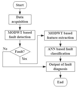
In the proposed scheme, there are three main parts: the fault detection, feature extraction, and fault classification. Firstly, the fault data are obtained from different fault conditions. Secondly, the fault detection is performed based on MODWT, and it aims to determine whether and when the fault occurs. Thirdly, the feature vectors are extracted through MODWT, then, they are put into the neural network for training. Finally, the results of the fault classification can be obtained. The flow chat of the proposed scheme is given in Figure 1.
Figure 1. The flow chat of the fault diagnosis scheme
2.1 MODWT based fault detection
2.1.1 Maximum overlap discrete wavelet transform
Compared with DWT, MODWT has the following characteristics [13]: it can handle any sample size N with a wider range of applicability; besides, it has no down-sampling process, and wavelet coefficients can be calculated immediately after each sampling process; what’s more, MODWT is not affected by the starting point of the time series, and it is different from DWT.
For a signal $Y(n)$ of any length N, MODWT decomposes the signal into $\log _{2} N$ levels. Meanwhile, the wavelet coefficients $\widetilde{W}_{j, n}$ and scale coefficients $\tilde{V}_{j, n}$ of the $j^{t h}$ level are shown in Eqns. (1) and (2):
$\widetilde{W}_{j, n}=\sum_{l=0}^{L_{j}-1} \tilde{h}_{j, l} Y_{n-l \bmod N}$ (1)
$\tilde{V}_{j, n}=\sum_{l=0}^{L_{j}-1} \tilde{g}_{j, l} Y_{n-l \bmod N}$ (2)
$n=0,1,2, \ldots, N-1$, where, N is the signal’s sampling length; $\tilde{h}_{j, l}$ is the wavelet filter the $j^{t h}$ stage; $\tilde{g}_{j, l}$ is the scale filter of the $j^{t h}$ stage; $L_{j}$ is the filter’s width of the $j^{t h}$ level. For more details, please refer to the papers [13, 16].
2.1.2 Detection algorithm
After obtaining the data, the fault detection is carried on to judge whether a fault occurs. If a fault occurs, the current will undergo a sudden change, and generate a short transient phenomenon. By extracting and analyzing the high-frequency components in the first-level coefficients of MODWT, the time when the fault occurs can be detected, otherwise it ends.
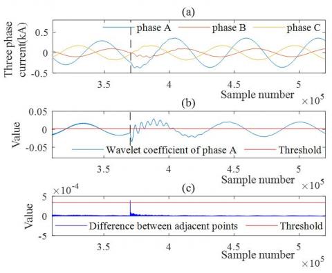
The modular extremum method is proposed by Silva at al. [18], that is, if the first-level wavelet coefficients exceed the set threshold, the occurrence time of the fault can be identified. However, the approach suffers the difficulty of choosing the appropriate threshold. If the threshold is set inappropriately, there will also be multiple points before the fault occurs that exceed the threshold, as shown in Figure 2(b). As a result, the detection fails.
Therefore, in order to improve the fault detection rate, the real-time fault detection in this article has made some adjustments to the technique of literature [18], which is mainly based on the adaptive threshold selection. An example that the comparison result of the two detection methods is represented in Figure 2.
Figure 2. An example of the comparison result of the two detection methods: (a) three-phase current of AG fault; (b) the detection result of the algorithm proposed in literature [18]; (c) the detection result of the algorithm proposed in this paper
The algorithm of the fault detection is as follows:
1) MODWT on the current using “ Haar ” wavelet;
2) The first-level detail coefficients of each phase are extracted, and the first 1000 and last 1000 detail coefficients are removed;
3) For the coefficients obtained in (2), first the difference between adjacent points in absolute value are calculated, which is defined as the Eq. (3). Then, the maximum value $D_{\mathrm{kmax}}$ of each phase are compared, and found.
$D_{k}=\left|C_{1, k+1}-C_{1, k}\right|$ (3)
where, $C_{1, k}$ is the $k^{t h}$ wavelet coefficient of the first level.
4) 2 points around $D_{\text {kmax }}$ of each phase are averaged, the maximum mean $D_{t h}$ and its phase are compared, and found.
$D_{t}=\frac{1}{3} \sum_{k \max -1}^{k \max +1} D_{k \max }$ (4)
5) The $D_{k}$ of the phase determined in (4) are compared with $D_{t h}$. If it is greater than $D_{t h}$, then it is related to the occurrence time of the fault.
As is seen in Figure 2, the algorithm proposed in this paper has achieved a good effect of detecting the fault, because there is only one point exceed the threshold, and the moment corresponding to this point is just the moment when the fault occurs. However, the method proposed in the literature [18] fails, because there are multiple points before the fault occurs that exceed the threshold, and the moment when the fault happens cannot be accurately determined. Besides, faults can also be detected at any time without delay. As for the accuracy of the detection results, we will discuss with the results of fault classification.
2.2 Feature extraction
After detecting the faults, two successive cycles of the currents are used as the objects for feature extraction, and it starts from the previous cycle of the faults. Then, the detail coefficients of each level are obtained after MODWT. However, if the detail coefficients are directly employed as feature vectors for training, it will result large memory space, long processing time, and poor classification accuracy [19]. Therefore, on the premise of not losing the original signal characteristics, it is vital to choose the appropriate feature vectors for training [20]. In this paper, “change in total standard deviation” and “change in the sum of mean” are calculated as the neural network’s inputs. The details of the feature vectors are as follows:
1) Standard Deviation: it is typical that standard deviation is utilized as the feature vector, which can reflect the degree of dispersion of a set of data distribution. The definitions of total standard deviations and change in total standard deviations are indicated in Eqns. (5) and (6):
$\sigma_{D}=\sum_{i=1}^{J} \sqrt{\frac{1}{N} \sum_{j=1}^{N}\left(D_{i j}-\mu_{D, i}\right)^{2}}$ (5)
$\Delta \sigma_{D}=\sigma_{D A}-\sigma_{D B}$ (6)
where, $i=1,2,3, \ldots, J$ (J is the decomposition level of MODWT); N is the amount of sampling points at each level; $D_{i j}$ is the detail coefficient; $\mu_{D, i}$ is the mean of detail coefficients at each level; $\sigma_{D A}$ is the total standard deviation of the post cycle of the fault; $\sigma_{D B}$ is the total standard deviation of the previous cycle of the fault.
2) Mean: the formulas of sum of mean and change in sum of mean are as follows:
$\mu_{D}=\frac{1}{N} \sum_{i=1}^{J} \sum_{j=1}^{N} D_{i j}$ (7)
$\Delta \mu_{D}=\mu_{D A}-\mu_{D B}$ (8)
where, $i=1,2,3, \ldots, J$ (J is the decomposition level of MODWT); N is the number of sampling points of each level; $D_{i j}$ is the detail coefficient; $\mu_{D A}$ is the sum of mean of the post cycle of the fault; $\mu_{D B}$ is the sum of mean of the previous cycle of the fault.
In summary: the description of feature vectors (F1-F8) are as follows:
1) F1: change in the total standard deviation of phase A;
2) F2: change in the total standard deviation of phase B;
3) F3: change in the total standard deviation of phase C;
4) F4: change in the total standard deviation of zero sequence;
5) F5: change in the sum of mean of phase A;
6) F6: change in the sum of mean of phase B;
7) F7: the change in the sum of mean of phase C;
8) F8: change in the sum of mean of zero sequence.
For example, the feature patterns for different short circuit faults are represented in Figure 3.
Figure 3. The feature patterns for different short circuit faults
2.3 Artificial neural network
Artificial neural network is a processor with simple processing units, and it is similar to the brain in that it acquires knowledge from external processes through a learning process. The BP neural network is one of relatively mature neural networks, and its network structure can be constructed through the neural network toolbox of MATLAB.
As the input layer, it is intended to receive the data-processed feature vectors from the outside world. In this paper, the input layer is determined by the 8-dimensional feature vectors (F1-F8), and the input is divided into training data set and test data set randomly. As the hidden layer, the aim is to convert the information into a targeted solution through internal self-learning and information processing, and the information is received by the input layer. The hidden layer’s output is given in Eq. (9):
$h_{j}=f\left(\sum_{i=1}^{n} w_{i j} x_{i}-b_{j}\right)$ (9)
where, n is the number of neurons in the input layer; $W_{i j}$ is the connection weight of the input layer and hidden layer; $j=1,2,3, \ldots, q$; q is the number of neurons in the hidden layer; $b_{j}$ is the threshold of hidden layer.
As the output layer, the intention is to get the final result by comparing the actual output with the expected output of the neuron. The output layer’s output is as follows:
$y_{k}=f\left(\sum_{k=1}^{m} v_{j k} h_{j}-t_{k}\right)$ (10)
where, $v_{j k}$ is the connection weight of the hidden layer and output layer; $k=1,2,3, \ldots, m$; m is the number of neurons in output layer; $t_{k}$ is the threshold of the output layer. In this paper, the output layer is determined by the 11 types of short-circuit faults. The classification of short-circuit faults is a binary classification problem, so the outputs can be expressed in binary mode, and it is given in Table 1.
Table 1. The binary mode of the outputs
|
Fault types |
Phase A |
Phase B |
Phase C |
Ground |
|
AG |
1 |
0 |
0 |
1 |
|
BG |
0 |
1 |
0 |
1 |
|
CG |
0 |
0 |
1 |
1 |
|
AB |
1 |
1 |
0 |
0 |
|
AC |
1 |
0 |
1 |
0 |
|
BC |
0 |
1 |
1 |
0 |
|
ABG |
1 |
1 |
0 |
1 |
|
ACG |
1 |
0 |
1 |
1 |
|
BCG |
0 |
1 |
1 |
1 |
|
ABC |
1 |
1 |
1 |
0 |
|
ABCG |
1 |
1 |
1 |
1 |
As a result, the diagram of ANN structure used for classification is given in Figure 4.
It is critical to set the learning parameters of the neural network, because there will be problems of over-fitting and under-fitting without proper selection of parameters. Usually it has no definite choice, and it can be set by empirical formulas and continuous experiments. This paper chooses the relatively best learning parameters through continuous experiments. Its learning parameters are illustrated in Table 2.
Table 2. ANN structure and learning parameters setting
|
Structure and parameters |
Values |
|
Input layer |
8 |
|
Hidden layer |
18 |
|
Output layer |
4 |
|
Training function |
traingdm |
|
Learning rate |
0.02 |
|
Training accuracy |
0.0001 |
|
Activation function |
Tangent,sigmoid |
3.1 Test system
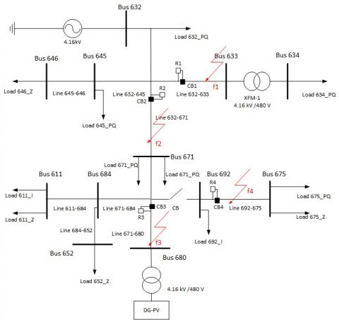
In this paper, the IEEE-13 bus system is adopted as the test system, which is a typical three-phase unbalanced system [21]. The test system is modelled in MATLAB, and its diagram is given in Figure 5. Referring to [22-23], the descriptions of the system are as follows:
1) It is a small 4.16 kV feeder system with high loads, and there is a 4.16 kV/480V transformer between lines 633-634;
2) The phases of the overhead and ground cables are unbalanced. Note that some are single-phase, such as lines 684-653 and 684-611; some are two-phase, like lines 671-684, 632-645, and 645-646; and others are three-phase;
3) A 4.16 kV three-phase voltage source is directly connected to node 632 in test system; however, a voltage regulator is connected from nodes 650 to nodes 632 in the original system;
4) The photovoltaic power generation unit is connected to the node 680 through a 4.16 kV/480 V transformer, in order to achieve grid connection;
5)The rest of the data are from the official website without any change. For specific parameters, please refer to literature [21].
Figure 4. Schematic diagram of BP network structure
Figure 5. Diagram of modified IEEE13 bus test system
This paper mainly focuses on the short-circuit fault, and its waveform can be captured through simulation. For example, the waveform of single-phase ground fault is depicted in Figure 6.
Figure 6. The waveform of single-phase ground fault
3.2 Data generation
In this study, different fault conditions with the change of electrical parameters are needed to be considered, and their specific settings are as follows:
1) Time of fault occurrence (initial phase angles of faults): the time of fault occurrence are usually consistent, and the initial angles of faults are set with a certain angular interval during simulation, such as literature [5, 10, 18]. However, the occurrence time and the initial angles of the faults are arbitrary, so there are certain limitations of the setting. In this study, three moments t1, t2, t3 that the faults occur were randomly generated during simulation, and they obey the uniform distribution on [0, 1];
2) Fault lines: line632-633, line632-671, line692-675, line671-680 in Figure 5;
3) Transition resistances: 0.01Ω, 1Ω, 50Ω;
4) Fault types: AG, BG, CG, AB, AC, BC, ABC, ABCG, ABG, ACG, BCG.
As a result: a total of $3 * 3 * 4 * 11=396$ fault conditions can be simulated.
3.3 Results of the proposed scheme
In order to verify the effectiveness of the proposed scheme, relevant sample data are obtained to test and evaluate it. First, all sample data are tested, and part of the output results are shown in Table 3. Then the recognition rate of fault detection and the accuracy rate of fault classification are counted, respectively. Additionally, the sample data of 4 lines are tested separately, and their classification accuracy are summarized. The fault diagnosis performance of the scheme is given in Table 4.
In the actual output result of the neural network, there is rarely a result that is exactly zero or one on each output neuron. Thus, if the error of each output neuron is within a small range, it can be ignored, and the fault is considered to be correctly classified [24]. As seen in Table 3, the error of each output neuron is almost within 0.03, and there are also few large errors. But in general, the errors can be ignored, the results of the actual output are satisfactory, and 11 types of the short-circuit faults are correctly identified.
Table 3. Part of the output results
|
Fault type |
Expected output |
Actual output |
|||
|
Phase A |
Phase B |
Phase C |
Ground |
||
|
AG |
(1 0 0 1) |
0.9994 |
0.0222 |
0.0404 |
0.9996 |
|
BG |
(0 1 0 1) |
0.0138 |
0.9980 |
0.0176 |
0.9916 |
|
CG |
(0 0 1 1) |
0.0168 |
0.0023 |
0.9802 |
0.9939 |
|
AB |
(1 1 0 0) |
0.9921 |
0.9877 |
0.0017 |
0.0157 |
|
AC |
(1 0 1 0) |
0.9898 |
0.0088 |
0.9878 |
0.0084 |
|
BC |
(0 1 1 0) |
0.0030 |
0.9904 |
0.9884 |
0.0024 |
|
ABG |
(1 1 0 1) |
0.9869 |
0.9954 |
0.0307 |
0.9798 |
|
ACG |
(1 0 1 1) |
0.9996 |
0.0018 |
0.9880 |
0.9977 |
|
BCG |
(0 1 1 1) |
0.0160 |
0.9976 |
0.9728 |
0.9917 |
|
ABC |
(1 1 1 0) |
0.9714 |
0.9805 |
0.9324 |
0.1896 |
|
ABCG |
(1 1 1 1) |
0.9916 |
0.9856 |
0.9972 |
0.9519 |
Table 4. Fault diagnosis results of the proposed scheme
|
Line |
Test data (groups) |
Accuracy |
|
|
Fault detection |
Fault classification |
||
|
Line632-633 |
99 |
100% |
99.51% |
|
Line632-671 |
99 |
100% |
97.75% |
|
Line671-680 |
99 |
100% |
98.92% |
|
Line692-675 |
99 |
100% |
98.47% |
|
Overall |
396 |
100% |
98.57% |
It can be concluded from Table 4 that the proposed algorithm of fault detection can detect all faults, and the recognition rate of fault detection can reach 100%. Consequently, the results of the fault detection prove that the algorithm is feasible. As for the performance of fault classification, it is slightly worse. Nevertheless, the approach can still offer a satisfactory overall classification accuracy of 98.57%, and it indicates that the method can successfully classify faults in most conditions. In addition, the accuracy of fault classification for different transmission lines can achieve more than 97.5%, and it shows that the method can adapt well to the change of parameters.
Although the proposed scheme can obtain a good classification accuracy, there are still individual misjudgments. The misjudgments exist because when the transition resistance increases, the characteristics of the voltage and current of the fault phase will become less and less obvious. And if the characteristics of the fault phase are less obvious, it will lead to the increased difficulty in distinguishing [16]. Especially in the case of high impedance (severe) faults, there may even be indistinguishable situations.
3.4 Comparison with other intelligent fault classification schemes
The performance of the proposed scheme with other intelligent fault diagnosis schemes are also compared, and results are summarized in Table 5. In addition, the best performing item is shown in bold. It should be noted that other schemes conclude two main parts: the methods in other studies and other algorithms. Moreover, the data of these comparison schemes are provided from the test system in this paper. And the faults are also detected with the method proposed in this paper, so they can all identify the faults. Besides, the method in scheme 2 refers to the reference [24].
Table 5. Comparison of the results with other schemes
|
Scheme |
Accuracy |
|
Proposed scheme |
98.57% |
|
DWT MRA+ANN [24] |
97.86% |
|
MODWT+SVM |
97.3% |
|
MODWT+DT |
97.22% |
|
MODWT+KNN |
96.5% |
From the comparison of fault diagnosis results in Table 5, in general, among all these comparison schemes, the proposed method outperforms the existing methods presented in Table 5 with the highest classification accuracy, so the results show that the proposed method is practicable to be applied to the fault diagnosis of the grids. In detail, on the one hand, the proposed scheme is compared with the method proposed in the literature [24], and the main differences between two methods are the selected wavelets and feature vectors. However, the proposed scheme in fault classification performs better than the other one, so the results infer that the choice of wavelet and feature vectors plays an important role in fault classification. On the other hand, the proposed scheme is compared with other algorithms, and the main difference between these methods is the artificial intelligence technology. However, the proposed scheme in fault classification performs better than others, so the results imply that the choice of artificial intelligence technology is also vital in fault classification.
An intelligent method of fault diagnosis in distributed power grids is shown in this paper, and the method is based on MODWT and ANN. First, fault detection is performed on the collected fault data. After identifying the faults, then the frequency domain features are extracted as feature quantities through MODWT, and finally the feature quantities are put into the artificial neural network for training. In order to verify the performance of the proposed scheme, it is tested on the simulation model of the modified IEEE-13 bus standard system. The results indicate that it can precisely detect faults, classify the fault types, and is not subjected to the variation of the electrical parameters. Meanwhile, contrasted with several existing diagnosis schemes, the proposed approach can provide better fault classification accuracy. Besides, future work will focus on the fault location and the optimization of neural network parameters.
[1] Blaabjerg, F., Yang, Y.H., Yang, D.S., Wang, X.F. (2017). Distributed power-generation systems and protection. Proceedings of the IEEE, 105(7): 1311-1331. https://doi.org/10.1109/JPROC.2017.2696878
[2] Gupta, P., Swarnkar, P. (2020). A new approach towards integration of multi-frequency, multi-voltage intertied hybrid power system. European Journal of Electrical Engineering, 22(3): 241-253. https://doi.org/10.18280/ejee.220305
[3] Kar, S., Samantaray, S.R. (2014). Time-frequency transform-based differential scheme for microgrid protection. IET Generation Transmission & Distribution, 8(2): 310-320. https://doi.org/10.1049/iet-gtd.2013.0180
[4] Said, B.M., Eddine, K.D., Salim, C. (2020). Artificial neuron network based faults detection and localization in the high voltage transmission lines with Mho distance relay. Journal Européen des Systèmes Automatisés, 53(1): 137-147. https://doi.org/10.18280/jesa.530117
[5] Manohar, M., Koley, E. (2017). SVM based protection scheme for microgrid. International Conference on Intelligent Computing, Instrumentation and Control Technologies (ICICICT), Kannur, India, pp. 429-432. https://doi.org/10.1109/ICICICT1.2017.8342601
[6] Kiaei, I., Lotfifard, S. (2019). Fault section identification in smart distribution systems using multi-source data based on fuzzy petri nets. IEEE Transactions on Smart Grid, 11(1), 74-83. https://doi.org/10.1109/TSG.2019.2917506
[7] Gao, Z.W., Cecati, C., Ding, S.X. (2015). A survey of fault diagnosis and fault-tolerant techniques-part II: Fault diagnosis with knowledge-based and hybrid/active approaches. IEEE Transactions on Industrial Electronics, 62(6): 3768-3774. https://doi.org/10.1109/TIE.2015.2419013
[8] Banerjee, S., Bhowmik, P.S. (2020). Transient disturbances and islanding detection in micro grid using discrete wavelet transform. 2020 IEEE Calcutta Conference (CALCON), Kolkata, India, pp. 396-401. https://doi.org/10.1109/CALCON49167.2020.9106498
[9] Perera, N., Rajapakse, A.D. (2012). Development and hardware implementation of a fault transients recognition system. IEEE Transactions on Power Delivery, 27(1): 40-52. https://doi.org/10.1109/TPWRD.2011.2174163
[10] Abdullah, A. (2018). Ultrafast transmission line fault detection using a DWT based ANN. IEEE Transactions on Industry Applications, 54(2): 1182-1193. https://doi.org/10.1109/TIA.2017.2774202
[11] Yu, J.J.Q., Hou, Y.H., Lam, A.Y.S., Li, V.O.K. (2019). Intelligent fault detection scheme for microgrids with wavelet-based deep neural networks. IEEE Transactions on Smart Grid, 10(2): 1694-1703. https://doi.org/10.1109/TSG.2017.2776310
[12] Huang, J.S., Jiang, Z.H., Rylands, L., Negnevitsky, M. (2018). SVM-based PQ disturbance recognition system. IET Generation Transmission & Distribution, 12(2): 328-334. https://doi.org/10.1049/iet-gtd.2017.0637
[13] Percival, D. B., Walden, A.T. (2000). Wavelet Methods for Time Series Analysis (Cambridge Series in Statistical and Probabilistic Mathematics). Cambridge University Press, Cambridge.
[14] Costa, F.B. (2014). Boundary wavelet coefficients for real-time detection of transients induced by faults and power-quality disturbances. IEEE Transactions on Power Delivery, 29(6): 2674-2687. https://doi.org/10.1109/TPWRD.2014.2321178
[15] Costa, F.B., Souza, B.A., Brito, N.S.D. (2010). Real-time detection of fault-induced transients in transmission lines. Electronics Letters, 46(11): 753-755. https://doi.org/10.1049/el.2010.0812
[16] Kar, S., Samantaray, S.R. (2016). High impedance fault detection in microgrid using maximal overlapping discrete wavelet transform and decision tree. International Conference on Electrical Power & Energy Systems (ICEPES), Bhopal, pp. 258-263. https://doi.org/10.1109/ICEPES.2016.7915940
[17] Jain, R., Du, Y.H., Lukic, S., Lubkeman, D. (2017). Fault identification in distribution systems using maximum overlap wavelet decomposition. 2017 North American Power Symposium (NAPS), Morgantown, WV, pp. 1-6. https://doi.org/10.1109/NAPS.2017.8107297
[18] Silva, K.M., Souza, B.A., Brito, N.S.D. (2006). Fault detection and classification in transmission lines based on wavelet transform and ANN. IEEE Transactions on Power Delivery, 21(4): 2058-2063. https://doi.org/10.1109/TPWRD.2006.876659
[19] Jayamaha, D.K.J.S., Lidula, N.W.A., Rajapakse, A.D. (2019). Wavelet-multi resolution analysis based ann architecture for fault detection and localization in dc microgrids. IEEE Access, 7: 145371-145384. https://doi.org/10.1109/ACCESS.2019.2945397
[20] Lidula, N.W.A., Rajapaks, A.D. (2012). A pattern-recognition approach for detecting power islands using transient signals-part ii: Performance evaluation. IEEE Transactions on Power Delivery, 27(3): 1071-1080. https://doi.org/10.1109/TPWRD.2012.2187344
[21] Kersting, W.H. (2001). Radial distribution test feeders. IEEE Power Engineering Society Winter Meeting. Conference Proceedings (Cat. No.01CH37194), Columbus, OH, USA, pp. 908-912. https://doi.org/10.1109/PESW.2001.916993
[22] Amraee, T., Mohammadnian, Y., Soroudi, A. (2019). Fault detection in distribution networks in presence of distributed generations using a data mining driven wavelet transform. IET Smart Grid, 2(2): 163-171. https://doi.org/10.1049/iet-stg.2018.0158
[23] Sharma, R., Mahela, O.P., Agarwal, S. (2018). Detection of power system faults in distribution system using stockwell transform. 2018 IEEE International Students' Conference on Electrical, Electronics and Computer Science (SCEECS), Bhopal, pp. 1-5. https://doi.org/10.1109/SCEECS.2018.8546879
[24] Li, W.L., Monti, A., Ponci, F. (2014). Fault detection and classification in medium voltage DC shipboard power systems with wavelets and artificial neural networks. IEEE Transactions on Instrumentation & Measurement, 63(11): 2651-2665. https://doi.org/10.1109/TIM.2014.2313035