Ghania Boudechiche* | Mustapha Sarra | Oualid Aissa | Jean-Paul Gaubert | Boualam Benlahbib | Abderezak Lashab
© 2020 IIETA. This article is published by IIETA and is licensed under the CC BY 4.0 license (http://creativecommons.org/licenses/by/4.0/).
OPEN ACCESS
This paper deals with a shunt active power filter (SAPF) integrated in a photovoltaic (PV) system, which is interfaced to the grid via a double-stage configuration, for simultaneously improving the power quality in the existence of non-linear loads and injecting the PV harvested power to the power grid. The direct power control (DPC) based on the conventional Proportional-integral (PI) suffers from some shortcomings in the transient state, such as large overshoots and undershoots in the voltage. Long response time is another disadvantage when using such a controller. To overcome this situation, the proposed control method is equipped by an anti windup fractional order proportional-integral differentiator (AW-FOPID) regulator, replacing the standard PI or PID regulators to maintain the DC link voltage at its desired value with small overshoots and undershoots in the voltage, while maintaining a short response time. The AW-FOPID controller, however, has five parameters, which makes it troublesome to tune. Accordingly, to adjust this AW-FOPID parameters, the Particle Swarm Optimization (PSO) algorithm is employed by minimizing the Integral Time Absolute Error (ITAE). Furthermore, an intelligent algorithm for tracking the maximum power point (MPPT) based on fuzzy logic has been applied to eventually resolve the drawback of the rapidly changing weather conditions. The overall control scheme is examined by simulation using MATLAB/Simulink software. The obtained simulation results and comparative study demonstrate the feasibility and performance of this control strategy.
direct power control, shunt active power filter, AW-FOPID controller, particle swarm optimization, fuzzy logic MPPT controller
So far, most of the world's energy is generated from fossil fuels (coal, oil, and gas), where these energy sources contribute to harmful gas emissions which are heavily involved in the global warming, as well as inducing pollution of the earth and organisms [1]. Furthermore, the excessive consumption of energy by these resources systematically leads to reduction of reserves of this kind of energy potential. Moreover, energy production is still a challenge of a great importance for the coming years since it is continually employed almost everywhere, i.e., in residential, commercial, and industrial areas. A good alternative is the power generation from renewable energies such as hydroelectric, geothermal, biomass, wind, and photovoltaic (PV), which operate without pollution effects on the atmosphere after use [2]. The availability of solar energy as an environment-friendly, unlimited, and free energy on the entire globe surface [3] has prompted researchers to select it among other existing sources of renewable energy for study and investigation. Meanwhile, the rapid growth of nonlinear loads integration causes problems in the electrical grids, such as reactive power and harmonic currents [4, 5]. Active power filters (APF) are the most resorted to solution for reducing the negative repercussions of such loads in the electrical grids [5]. Within the APF family, the shunt active power filter (SAPF), which is paralleled to the grid to inject a current that is opposing both the current harmonics and reactive power emitted by the load, to eventually make the current supplied by the electrical power system sinusoidal and in phase with its voltage, is commonly opted [6, 7]. An interesting combination would be to integrate a SAPF in a PV system to harvest their granular features mentioned above, all together [8, 9]. In the literature, many techniques have been presented to control the APF. Direct power control (DPC) is invented by Noguchi et al. in 1998 whose idea is inspired from the direct torque control (DTC) intended for electrical machines drives [5, 10]. The DPC method does not require current control loops or pulse-width-modulator (PWM) block. The switching table based on the correction of the reactive and active powers, as well as based on the sector indicating the angular position of the source voltage vector, is intended to select the switching states of the converter [11, 12]. In this context, researchers gave great importance to this table which was treated by Boukezata et al. [8] to achieve good performance of the DPC control. In most cases, the DPC is fed by a reference of zero reactive power and active one produced via the Proportional-Integral (PI) regulator of the converter dc-link voltage [5, 8]. Various control techniques are employed to maintain this latter at its reference value optimally, regardless of the operating conditions. Among those, the conventional PI controller is simple to implement and presents a good response in steady state [13, 14]. This controller, however, exhibits poor performance during dynamic conditions, which are in the case of SAPF integrated in a PV system start-up, changing solar irradiance, and changing load.
To overcome this situation, the proposed control in this paper is carried out by an anti windup fractional order proportional-integral differentiator AW-FO($\mathrm{P} \mathrm{I}^{\mathscr{E}} \mathrm{D}^{\eta}$) controller, replacing the standard PI regulator that keeps the DC bus voltage at its desired value. The benefits offered by this AW-FO($\mathrm{P} \mathrm{I}^{\mathscr{E}} \mathrm{D}^{\eta}$) regulator with two extra freedom degrees ℰ and η allows having better dynamic response and shorter response time compared to the conventional PI controller [15-17]. Moreover, the output of the proposed AW-FOPID controller effectively participates in the delivery of the active power compared to the standard PI regulator employed in DPC that suffers from weak responses in dynamic mode. Indeed, this is the first time that the AW-FOPID controller requiring the determination of five optimized parameters has been incorporated into the DPC. Regarding the adjustment of this AW-FOPID parameters, Particle Swarm Optimization (PSO) algorithm is used to minimize the Integral Time Absolute Error (ITAE) [18].
As the solar insolation varies, the voltage corresponding the maximum power point (MPPT) varies. Therefore, several algorithms of MPPT such as incremental conductance (IC), perturb and observe (P&O), and hill climbing (HC) have been proposed in the literature [19, 20]. The advantages offered by these aforementioned algorithms reside in the ease of calculation and implementation. Due to the deficiencies of the aforementioned algorithms especially during dynamically changing weather conditions, intelligent controllers like fuzzy logic has been used in tracking effectively the maximum power point (MPPT) in PV systems, whatever abrupt changes affecting solar irradiance and temperature [9, 21]. On the other hand, the design of fuzzy MPPT proposed in this paper is not subject to well-defined criteria but is mainly based on experience.
This paper is sectioned in the following way: Description of the operating principle of the SAPF is explained in Section 2; The principle of the DPC applied to the SAPF together with PSO tuned AW-FO($\mathrm{P} \mathrm{I}^{\mathscr{E}} \mathrm{D}^{\eta}$) controller design to regulates the DC-link voltage, and fuzzy logic controller (FLC) for tracking the maximum power point, are presented in Section 3. Simulation results are given and discussed in Section 4. Finally, the presented work is concluded in Section 5.
APFs are, in simple words, systems that are used to eliminate the harmonics pollution along the power line caused by the non linear loads, as well as the reactive power induced by those loads, regardless of their nature [5]. The voltage source connected in parallel with the non-linear load, becomes nearly sinusoidal because the SAPF injects harmonics current with the same amplitude and opposite in phase to the load’ sone. Regarding the reactive power, it is compensated by injecting filtering current with a phase that is opposed to the line’s current one [12, 22].
Figure 1. Simplified schematic of the SAPF
Figure 1 shows a simplified schematic of a SAPF. According to this figure, the source’s current can be expressed in the following form
${{I}_{s}}={{I}_{1}}+{{I}_{f}}$ (1)
where Is is the source current; Il is the load current; and If is the compensation current.
3.1 Direct power control
The basic principle of DPC was proposed by Noguchi [11], while it was initially inspired from the DTC of electric motors control [23]. In the DPC strategy, reactive and active powers imitate, respectively, the electromagnetic torque and the amplitude of the stator flux of the DTC. This non-linear method is known as a direct power control technique because it chooses the optimal voltage vector without need for any modulation technique or coordinates transformation. The basic concept of the DPC is to select the appropriate states from the switching table based on localisation of the source voltage vector and errors [22-24].
In the proposed DPC method, the continuous bus voltage is maintained at the desired level through an AW-FOPID regulator-based voltage regulation loop.
The instantaneous active and reactive powers are calculated starting from the following equations:
${{P}_{s}}={{V}_{sa}}{{I}_{sa}}+{{V}_{sb}}{{I}_{sb}}+{{V}_{sc}}{{I}_{sc}}$ (2)
${{Q}_{s}}=\frac{1}{\sqrt{3}}\left[ \left( {{V}_{sb}}-{{V}_{sc}} \right){{I}_{sa}}+\left( {{V}_{sc}}-{{V}_{sa}} \right){{I}_{sb}}+\left( {{V}_{sa}}-{{V}_{sb}} \right){{I}_{sc}} \right]$ (3)
${{S}_{s}}={{P}_{s}}+j{{Q}_{s}}$ (4)
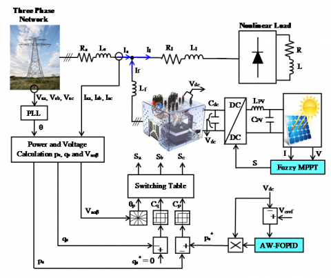
The reference of the reactive power is set to zero value to ensure a unity power factor. Whereas, the reference of the active power is developed with the multiplication of the peak value of the current source generated by the AW-FOPID regulator and the optimal value of the PV generator voltage. Then, the powers are compared and the obtained errors are applied to the hysteresis regulators [9, 22, 24]. The used hysteresis regulators allow restricting the errors of the instantaneous reactive and active powers in the desired band, as shown in Figure 2. The output of the controller switches between 1 and 0, where it is 1 if the error is positive and 0 otherwise. The influence of each control vector applied to the APF on the reactive and active powers is dependent on the actual position of the source voltage vector. Thus, the switching Table 1 has as inputs the signals from both hysteresis comparators and the information on the source voltage vector.
Figure 2. General structure of SAPF controlled by the proposed DPC approach in presence of the PV system
Table 1. Switching table of DPC strategy
|
$C_{p}$ |
$C_{q}$ |
$\boldsymbol{\theta}_{1}$ |
$\boldsymbol{\theta}_{2}$ |
$\boldsymbol{\theta}_{3}$ |
$\boldsymbol{\theta}_{4}$ |
$\boldsymbol{\theta}_{5}$ |
$\boldsymbol{\theta}_{6}$ |
$\boldsymbol{\theta}_{7}$ |
$\boldsymbol{\theta}_{8}$ |
$\boldsymbol{\theta}_{9}$ |
$\boldsymbol{\theta}_{10}$ |
$\boldsymbol{\theta}_{11}$ |
$\boldsymbol{\theta}_{12}$ |
|
1 |
1 |
$v_{6}$ |
$v_{7}$ |
$v_{1}$ |
$v_{0}$ |
$v_{2}$ |
$v_{7}$ |
$v_{3}$ |
$v_{0}$ |
$v_{4}$ |
$v_{7}$ |
$v_{5}$ |
$v_{0}$ |
|
1 |
0 |
$v_{7}$ |
$v_{7}$ |
$v_{0}$ |
$v_{0}$ |
$v_{7}$ |
$v_{7}$ |
$v_{0}$ |
$v_{0}$ |
$v_{7}$ |
$v_{7}$ |
$v_{0}$ |
$v_{0}$ |
|
0 |
1 |
$v_{6}$ |
$v_{1}$ |
$v_{1}$ |
$v_{2}$ |
$v_{2}$ |
$v_{3}$ |
$v_{3}$ |
$v_{4}$ |
$v_{4}$ |
$v_{5}$ |
$v_{5}$ |
$v_{6}$ |
|
0 |
0 |
$v_{1}$ |
$v_{2}$ |
$v_{2}$ |
$v_{3}$ |
$v_{3}$ |
$v_{4}$ |
$v_{4}$ |
$v_{5}$ |
$v_{5}$ |
$v_{6}$ |
$v_{6}$ |
$v_{1}$ |
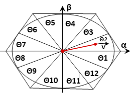
Figure 3. Sectors on stationary coordinates
According to the angle between the inverter output voltage reference and the α axis, the sector will be selected as shown in Figure 3. Consequently, the angle is determined by an inverse trigonometric function based on the vector components of the voltage in the fixed reference space (α, β):
${{\theta }_{p}}={{\tan }^{-1}}\left( \frac{{{v}_{s\beta }}}{{{v}_{sa}}} \right)$ (5)
p is the number of the sector. Accordingly the inverter output voltage reference is selected based on the desired reactive and active power values.
3.2 Particle swarm optimization (PSO) based fractional order $\mathrm{P} \mathrm{I}^{\mathscr{E}} \mathrm{D}^{\eta}$ controller design
3.2.1 AW-FOPID controller
The conventional PI controller suffers from some weakness in the dynamic state. To overcome this drawback, the proposed control is carried out by an AW-FOPID, replacing the standard PI regulator to keep the DC bus voltage at its desired value with shorter response time during dynamic conditions, while the overshoots and undershoots are maintained at minimum levels. The AW-FOPIεDη has been introduced in 1999 with its general form in which the integral and derivative action orders, ε and η respectively, are not integers [25], as shown in Figure 4. The AW-FOPID controller has good convergence and conservation of the adjusted variable to its desired value. Moreover, due to the better dynamic response, flexibility and low sensitivity to eventual variations of the system parameters, AW-FOPID controllers belong to the dominating industrial controllers which have attracted the attention of several researches in different fields, such as: aerospace control systems [26], hypersonic flight vehicle, and automatic voltage regulation [27-30].
Figure 4. AW-FOPID controller structure
From Figure 4, the transfer function G(s) of the AW-FOPID controller is calculated by the following equation:
$G\left( s \right)=\frac{U\left( s \right)}{E\left( s \right)}={{K}_{p}}+{{K}_{i}}{{s}^{-\varepsilon }}+{{K}_{d}}{{s}^{\eta }}$ (6)
where Kp, Ki, Kd are the proportional, integral and derivative gain factors, respectively; ε, η are the integral and derivative orders respectively; R(s) is the input signal; C(s) represents the plant’s transfer function; E(s) is the error signal and Y(s) is the output signal.
It can be noticed that the selection of $\varepsilon$, $\eta$ gives the conventional controllers, i.e. PID controller ($\varepsilon$, $\eta$=1), PD controller ($\varepsilon$=0) and PI controller ($\eta$=0).
(1) Approximation method of fractional order operators
The method proposed by Oustaloup [31] is more elaborated and more convenient to approximate the fractional order (FO) to Laplace transfer functions (TFs). The term sα of the Oustaloup’s approximation model is defined in the study [32], where s is the Laplace transform variable and α is a real number which ranges between -1 and 1. sα is designated as an FO differentiator if (0<α<1) and as an FO integrator (−1<α<0). Moreover, this method is called recursive Oustaloup's filter and it distributed in a limited frequency band [wb wh]. So, the approximate of the fractional order (FO) to Laplace transfer functions (TFs) is assessed as follows:
${{s}^{\alpha }}=K\prod\limits_{k=-N}^{N}{\frac{s+{{{{\omega }'}}_{k}}}{s+{{\omega }_{k}}}}$ (7)
where:
${{{\omega }'}_{k}}={{\omega }_{b}}{{\left( \frac{{{\omega }_{h}}}{{{\omega }_{b}}} \right)}^{\left( \frac{k+N+0.5(1-\alpha )}{2N+1} \right)}}$ (8)
${{\omega }_{k}}={{\omega }_{b}}{{\left( \frac{{{\omega }_{h}}}{{{\omega }_{b}}} \right)}^{\left( \frac{k+N+0.5(1+\alpha )}{2N+1} \right)}}$ (9)
$K=\omega _{h}^{\alpha }$ (10)
With ωk′ and ωk are respectively the zeros and poles of interval k; K represents the adjustment gain; ωb and ωh are respectively the low and high frequencies; N is the number of poles and zeros, and (2N+1) is the approximation function order.
(2) Particle swarm optimization (PSO)
According to (6), the AW-FOPID controller has five parameters to be adjusted (Kd, Kp, Ki, ℰ and η). To tune these parameters, the PSO algorithm is used by minimizing the objective function (F). PSO algorithm is a stochastic population-based computer algorithm to find an optimal solution to a problem. This technique was initially invented by Russel James Kennedy and Eberhart in 1995. It was developed based on the behaviour of some animals, such as fish and birds [28, 29]. In PSO algorithm, each individual is named “particle” which is considered as a candidate solution to find the optimal solution to the problem. A particle’s position is affected by its own best found position, as well as the position of the best particle in its neighbourhood. For the local best PSO, a smaller neighbourhoods are determined for each particle. Whereas in the global best PSO, the neighborhood for each particle is all particle’s of swarm (entire swarm).
The fitness function evaluates and quantifies the performance of a particle [28, 30]. The personal best position of the particle i is estimated as
${{y}_{i}}(t+1)=\left\{ \begin{align} & {{y}_{i}}(t)\text{ if F(}{{x}_{i}}(t+1)\ge F({{y}_{i}}(t)) \\ & {{x}_{i}}(t+1)\text{ if F(}{{x}_{i}}(t+1)\langle F({{y}_{i}}(t)) \\ \end{align} \right.$ (11)
With xi is the particle's current position; F is the objective function. This best position of the particle i is updated at time step t. For the global best position, y is defined as:
$y=\text{ min}\left\{ F \right.\text{(}{{\text{y}}_{0}}(t)),........,F({{y}_{s}}(t)\left. ) \right\}$ (12)
With s is the swarm’s size. The standard equations of PSO for each dimension j: jϵ {1,..., Nd } are given as:
${{v}_{i}}_{,j}\text{=}\omega \text{.}{{v}_{i}}_{,j}(t)+{{c}_{1}}.{{\Delta }_{1}}+{{c}{2}}.{{\Delta }_{2}}$ (13)
$\text{ }{{x}_{i}}(t+1)={{x}_{i}}(t)+{{V}_{i}}(t+1)$ (14)
where:
${{\Delta }_{1}}={{r}_{1,j}}.({{y}_{i,j}}(t)-{{x}_{i,j}}(t))\text{ }$ (15)
${{\Delta }_{2}}={{r}_{2,j}}.(y_{j}^{n}(t)-{{x}_{i,j}}(t))\text{ }$ (16)
vi, j is the jth element of the velocity vector of the ith particle, ω is the inertia weight, c1 and c2 are the acceleration constants, and r1,j , r2,j are random coefficients in the range [0, 1]. When the velocity updates tend to zero, this process is stopped.
Various optimization criteria are used for adjusting the process controllers. Among those, the minimization of Integral Time Absolute Error (ITAE):
$Min\text{ F}=Min[\int\limits_{0}^{\infty }{t\left| e(t) \right|}dt]$ (17)
The PSO algorithm used to design the AW-FOPID controller parameters is represented in Figure 5.
Figure 5. PSO-based AW-FOPID controller parameters design
In every iteration, each particle needs to update its own best individual fitness. The individual fitness of each particle is measured by using the Integral Time Absolute Error (ITAE) which can be expressed as:
$MSE=\frac{\sum\limits_{r=0}^{N}{{{e}^{2}}}}{N}$ (18)
where, N denotes the total number of points for which the optimization is carried out, ts is the time rang of simulation. In this study, PSO with the spreading factor (PSO-SF) [32-38] is used and modified so that the algorithm can be used to tune the AW-FOPID controller parameters. By using the spreading factor approach, the values of the acceleration coefficient and inertia weight can be linearly converged to the predefined values over time as illustrated by the following equations:
${{w}_{e}}={{e}^{(-current\text{ epoch/(SF}\times total\text{ epoch))}}}$ (19)
where: SF = 0.5(spread + deviation).
${{c}_{1}}={{c}_{2}}=2\times (1-(current\text{ epoch/total epoch))}$ (20)
The instructions to be followed by the algorithm of tuning process of AW-FOPID controller by PSO are given as follows:
1- Initialize the parameters and specify the lower and upper bounds of the five controller parameters: inertia weight (we) from 0 to 1, acceleration coefficients range (c1 and c2) from 0.05 to 2, position range from 0.01 to 15 and velocity range from -0.001 to 0.5;
2- Randomly distribute particles within specified ranges;
3- While current number of epochs is less than 1000;
4- Evaluate the fitness of each particle using Eq. (18) with MSE tends to 0;
5- If the current individual fitness is better than the previous individual fitness, then update new individual fitness;
6- Identify the best particle fitness among the swarm;
7- If the current population fitness is better than the previous population fitness, then update new population fitness;
8- Calculate the velocity and update the position using Eqns. (13) and (14) respectively;
9- Calculate the new values of the acceleration coefficients and the inertia weight using Eqns. (20) and (19) respectively;
10- End.
3.3 Fuzzy logic MPPT controller
3.3.1 Photovoltaic array model
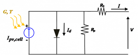
The photovoltaic array employed in the developed system is a KC200GT, characterized by a single diode model [33, 34]. From Figure 6, the equivalent circuit of the PV cell is illustrated by a current source in parallel with a diode and series/parallel resistors.
Figure 6. Electrical equivalent circuit of a PV cell
The current relation of the PV cell is represented by the next equation:
$I={{I}_{pv,cell}}-{{I}_{0,cell}}\left[ {{e}^{\left( \frac{qV}{aKT} \right)}}-1 \right]$ (21)
where:
${{I}_{pv}}=\left( {{I}_{pv,n}}+{{K}_{I}}{{\Delta }_{T}} \right)\frac{G}{{{G}_{n}}}$ (22)
Ipv,cell is the generated current by the incident light; I0,cell is the leakage current of the diode; K is Boltzmann’s constant, all measured in ampere [J.K-1]; T is the effective cell’s temperature, measured in Kelvin [K]; q is the electron’s charge, measured in Coulomb [C]; a is the non-ideal junction factor, measured in ampere; Ipv;n is the solar generated current at the nominal condition; ΔT=T-Tn (Tn and T is the nominal and actual temperatures, measured in Kelvin [K]; respectively); Gn(W/m2) is the nominal irradiation; G is the irradiation and KI is the short circuit current/temperature coefficient.
Considering the PV panel series and shunt resistors gives the following:
$I={{I}_{pv}}-{{I}_{0}}\left[ {{e}^{\left( \frac{q\left( V+I{{R}_{s}} \right)}{a{{N}_{s}}KT} \right)}}-1 \right]-\frac{V+I{{R}_{s}}}{{{R}_{p}}}$ (23)
where: Ns is the number of cells mounted in series. A practical PV array consists of many PV cells connected in series and in parallel. This is achieved by adding some the series and parallel coefficients as follows [35]:
$\begin{align} & I={{N}_{pp}}{{I}_{pv}}-{{N}_{pp}}{{I}_{0}}\left( {{e}^{\left( \frac{{{N}_{ss}}V+I{{R}_{s}}\left( {\scriptstyle{}^{Nss}/{}_{{{N}_{pp}}}} \right)}{{{N}_{ss}}\alpha {{V}_{t}}} \right)}}-1 \right) \,\,\,\,\,\,\,\,-\frac{{{N}_{ss}}V+I{{R}_{s}}\left( {\scriptstyle{}^{Nss}/{}_{{{N}_{pp}}}} \right)}{{{R}_{p}}\left( {\scriptstyle{}^{{{N}_{ss}}}/{}_{{{N}_{pp}}}} \right)} \\ \end{align}$ (24)
where: Nss is the number of PV panels mounted in series and Npp is the number of PV panels mounted in parallel.
3.3.2 Maximum power point tracking (MPPT)
(1) Fuzzy logic controller
Fuzzy logic method is employed for tracking the MPP of PV module to achieve good efficiency under any weather conditions. The fuzzy logic approach is very efficient for both linear and nonlinear controlled systems, while the mathematical model is not needed [9, 21].
Figure 7. Fuzzy logic controller block diagram
Generally, the FLC is executed in three essential steps: Fuzzification, Rules inference, and Defuzzificationas shown in Figure 7 [21, 36]. The Fuzzification step is the process of changing the digital input variables into linguistic equivalent, which are achieved by using membership functions. The Rules inference step determines the output of the fuzzy logic controller by Mamdani method with a max-min technique depending on the set belonging to the rule base. The Defuzzification step converts the linguistic variables into a crisp value which calculates the output control variable. Since at the MPP of the PV array, ΔP(k) and ΔV(k) are null, the proposed algorithm, therefore, has two input variables, which are based on Eqns. (25) and (26) [37]:
$\text{ }\!\!\Delta\!\!\text{ P}=\text{P}\left( \text{k} \right)-\text{P}\left( \text{k}-1 \right)$ (25)
$\text{ }\!\!\Delta\!\!\text{ V}=\text{V}\left( \text{k} \right)-\text{V}\left( \text{k}-1 \right)$ (26)
where: P(k), P(k-1), V(k), and V(k-1) are respectively, the PV power and voltage at the sampling times k and (k-1), respectively. These inputs of the fuzzy MPPT are represented by the error E and its variation ∆E [36, 37]:
$\left\{ \begin{align} & \text{E(k)}=\frac{\text{ }\!\!\Delta\!\!\text{ P}}{\text{ }\!\!\Delta\!\!\text{ V}} \\ & \text{ }\!\!\Delta\!\!\text{ E(k)}=\text{E(k)}-\text{E(k}-\text{1)} \\ \end{align} \right.$ (27)
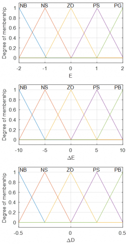
The input variables E(k) and ΔE(k) are divided into five fuzzy sets which are denoted as: Negative Big (NB), Negative Small (NS), Zero (ZO), Positive Small (PS), and Positive Big (PB). The rule base connects the fuzzy inputs to the fuzzy output by the master rule of syntax: '' if X and Y, then Z'' [9, 37], as listed in Table 2.
Table 2. Fuzzy logic decision table
|
E/∆E |
NB |
NS |
ZO |
PS |
PB |
|
NB |
PS |
PB |
PB |
NB |
NS |
|
NS |
ZO |
PS |
PS |
NS |
ZO |
|
ZO |
ZO |
ZO |
ZO |
ZO |
ZO |
|
PS |
ZO |
NS |
NS |
PS |
ZO |
|
PB |
NS |
NB |
NB |
PB |
PS |
Figure 8. Membership functions for inputs and output variables
For ease of calculation, equilateral triangle membership functions are chosen (Figure 8). The center of gravity method for defuzzification step is used to calculate the incremental duty cycle ΔD as [9, 37]:
$\Delta D=\frac{\sum\nolimits_{j=0}^{n}{{{w}_{j}}\Delta {{D}_{j}}}}{\sum\nolimits_{j=0}^{n}{{{w}_{j}}}}$ (28)
With: n is the maximum number of effective rules, w represents the weighting factor and ΔDj is the value corresponding to ΔD. Finally, the duty cycle is obtained by adding this change to the previous value of the control duty cycle as expressed in the following [37]:
$D\left( K+1 \right)=D\left( K \right)+\Delta D\left( K \right)$ (29)
To validate the feasibility and performance of the control technique proposed in this paper, various simulation tests under MATLAB/Simulink environment were conducted. The simulation model parameters used for these tests are presented in Tables 3 and 4.
Table 3. Simulation parameters
|
Parameters |
Values with dimensions |
|
Vs, Fs |
70 V, 50 Hz |
|
Fswitching (DC/AC APF converter) |
20 KHz |
|
Ls, Rs |
0.1 mH, 0.1 Ω |
|
Ll, Rl |
0.566 mH, 0.01 Ω |
|
Lf, Rf, Cdc |
2.5 mH, 0.01Ω, 2200 µF |
|
L, R |
10 mH, 40 Ω |
|
Cpv, Lpv |
20 µF, 3 mH |
|
DC bus voltage reference (Vcref) |
227.68 V |
|
Fswitching (DC/DC boost converter) |
5 kHz |
|
N |
2 |
|
ωb, ωh |
10-2 rad/s, 102 rad/s |
|
Kp, Ki, Kd |
0.95, 60, 0.011 |
|
$\mathscr{E}, \eta$ |
0.4, 0.5 |
|
Parameters |
Values with dimensions |
|
Swarm size |
10 |
|
Number of iterations |
100 |
|
r1, r2 |
0.1, 0.1 |
|
cl, c2 |
0.566, 0.01 |
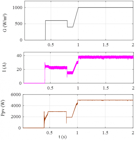
Figure 9 shows the adopted solar irradiance profile, along with the PV array power and current. Firstly, with null irradiation, no current and power are generated until 0.4s. Then, from 0.4s to 2s they follow their trajectories imposed by the applied irradiation profile. Consequently, the irradiance increases from 0 to 600W/m2 until 0.8s passes, providing 3kW with 25A by applying the FLC-based MPPT algorithm. At 0.8s, the solar irradiance decreases suddenly from 600 to 400W/m2 tailed by a power decrease from 3kW to 1.99kW with decreasing current from 25A to 15A. At 0.9s, the solar irradiance increases gradually until it reaches 1000W/m2 at 1s, and continues at this level until the end of the profile by generating 5kW with 40A. The harvested power under the whole profile is injected to the grid through the multifunctional SAPF, considering both control methods under test, i.e. the proposed AW-FOPID and its counterpart the PI and PID, all integrated into DPC.
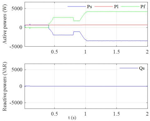
Figures 10, 13 and 16 show the active and reactive powers of the SAPF controlled using DPC with the standard PI, PID and AW-FOPID regulators, respectively, combined with FLC MPPT controller. When the irradiation is zero, the electrical network supplies all the power (Ps) to the load (Pl). After the PV array starts in the time interval [0.4, 2]s, the PV array simultaneously supplies the demanded power by the non-linear load and the rest of the energy (Pf) is transferred to the electrical network. During the time interval [0.1, 2]s, while the SAPF is inserted, the reactive power of the network (Qs) becomes null since the reactive power demanded by the load is compensated by the SAPF. While before filtering it was the grid who provides the reactive power to the non-linear load.
Figure 10. Active and reactive powers of the SAPF based on conventional DPC with the standard PI regulator integrated with fuzzy logic MPPT controller
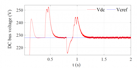
Figure 11. Zoomed-in view on DC bus voltage of the SAPF obtained by the conventional DPC with the standard PI regulator
(a)
(b)
(c)
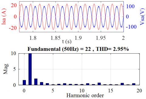
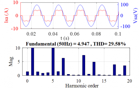
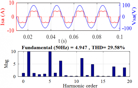
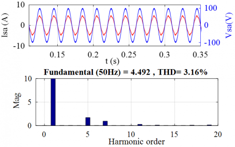
Figure 12. Source voltage and current with FFT of the latter of the SAPF based on the conventional DPC with the standard PI regulator: (a) without SAPF, (b) with SAPF and (c) with solar SAPF
Figure 13. Active and reactive powers of the SAPF based on conventional DPC equipped with the standard PID regulator and fuzzy logic MPPT controller
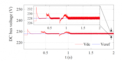
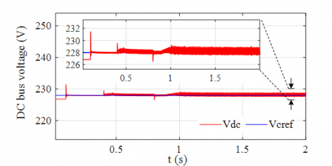
On the other hand, the DC bus voltage (Vdc) is regulated to its reference value (Vcref) during the insertion of the SAPF at the instant t = 0.1s, and it is supposed to be kept at Vcref even during irradiance variations due to the exchange of power between the grid, the non-linear load, and the APF, as shown in Figures 11, 14 and 17. During the time interval [0.1-0.4]s, where the solar irradiance equals to 0 w/m², it can be noticed that Vdc increases from 227.68V to 242.888V for PI, 232.578V for PID and 231.268V for AW-FOPID with response time 0.1186s, 0.08s and 0.00435s, respectively.
However, when the solar irradiance equals to 600W/m² during the time interval [0.4-0.8]s, it can be seen that Vdc increases from 227.68V to 252.788V for PI, 230.028V for PID and 229.248V for AW-FOPID with response time 0.225s, 0.12s and 0.0053s, respectively. Then, when the solar irradiance equals to 400W/m² during the time interval [0.8-0.9]s, it can be noticed that Vdc decreases from 227.68V to 215.008V for PI, 225.368V for PID and 226.209V for AW-FOPID with response time 0.114s, 0.08s and 0.0045s, respectively. Finally, in the time interval [0.9-2]s when the solar irradiance increases from 400 to 1000W/m², it can be observed that Vdc increases from 227.68V to 244.488V for PI, 229.668V for PID and 228.468 V for AW-FOPID with response time 0.261s, 0.15s and 0.00022s, respectively. Consequently, it is clear that the proposed AW-FOPID controller has a smaller overshoots and voltage drops with smaller response time during irradiation changes compared to its counterparts, the conventional PI and PID regulators, as shown in Figures11, 14, 17 and Table 5.
Figures 12, 15, 18, 19 and 20 show the waveforms of the source voltages (Vs) and currents (Is) along with their FFT analysis, the currents of the filter (If), and the currents of the load (Il). These variables are shown before and after filtering, and without and with PV array, together with their respective zooms. Before filtering and between 0s and 0.1s, the form of the source current is distorted and rich in harmonics, which are generated by the nonlinear load, as shown in Figures 12(a), 15(a), and 20(a).
Figure 14. Zoomed-in view on DC bus voltage of the SAPF obtained by the conventional DPC with the standard PID regulator
(a)
(b)
(c)
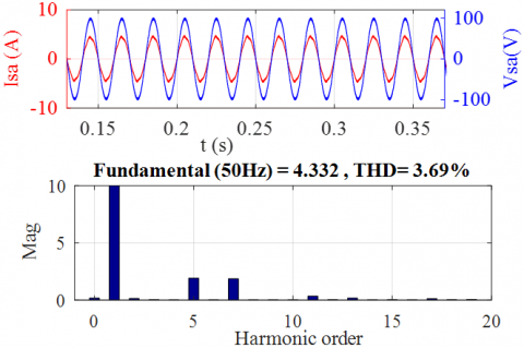
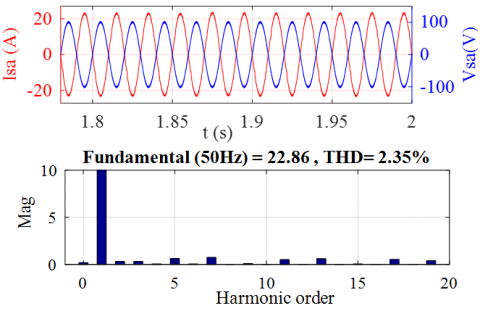
Figure 15. Source voltage and current with FFT of the latter of the SAPF based on conventional DPC equipped with the standard PID regulator: (a) without SAPF, (b) with SAPF and (c) with solar SAPF
Figure 16. Active and reactive powers of the SAPF based on proposed DPC with the AW-FOPID regulator associated with fuzzy logic MPPT controller
Figure 17. Zoomed-in view on DC bus voltage of the SAPF obtained by the conventional DPC with the proposed AW-FOPID regulator
Figure 18. Simulation results of the solar FAP based on proposed DPC equipped with the AW-FOPID regulator and fuzzy MPPT controller. Source voltages and currents, filter and load currents
Figure 19. Zoomed-in view on the simulation results of the SAPF based on proposed DPC with the AW-FOPID regulator associated with fuzzy MPPT controller: source voltages and currents, filter and load currents
(a)
(b)
(c)
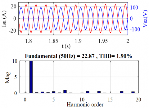
Figure 20. Source voltage and current with FFT of the latter of the SAPF based on proposed DPC with the AW-FOPID regulator: (a) without SAPF, (b) with SAPF and (c) with solar SAPF
The value of current total harmonics distortion (THD) was equal to 29.58%. However, the source current becomes sinusoidal and in phase with the network voltage after the insertion of the SAPF at 0.1s, where the THD decreased to 3.81% for the DPC with PI, 3.69% for the DPC with PID and 3.16% for the DPC with AW-FOPID, as shown in Figures 12(b), 15(b), and 20(b). Then from 0.4 to 2s, the SAPF is interfaced with the PV system.
From Figures 12(c), 15(c), and 20(c), it is worth to note that, the source current remains sinusoidal despite the change in the irradiation and is opposed in phase with the source voltages. Consequently, the THD is 2.95%, 2.35% and 1.9% for the conventional PI, PID and AW-FOPID regulators, respectively.
Table 5. Comparative study of the proposed AW-FOPID with conventional PI and PID controllers before and after introducing fuzzy logic MPPT controller
|
|
Recorded values in transient state for the dc bus voltage using the PI, PID, and AW-FOPID controller |
|||
|
|
SAPF without PV ΔV(V) |
SAPF without PV Δt (s) |
SAPF with PV ΔV(V) |
SAPF with PV Δt (s) |
|
Proposed DPC with AW-FOPID regulator |
Overshoot of 3.58 |
0.00435 |
Overshoot of 1.56 Voltage drop of 1.479 Overshoot of 0.78 |
0.0053 0.0045 0.00022 |
|
Conventional DPC with PID regulator |
Overshoot of 4.89 |
0.08 |
Overshoot of 2.34 Voltage drop of 2.32 Overshoot of 1.98 |
0.12 0.08 0.15 |
|
Conventional DPC with standard PI regulator |
Overshoot of 15.2 |
0.1186 |
Overshoot of 25.1 Voltage drop of 12.68 Overshoot of 16.8 |
0.225 0.114 0.261 |
In this paper, a DPC based on AW-FOPID regulator for a multifunctional PV system integrated into the grid is proposed. This AW-FOPID regulator parameters are optimized by using PSO algorithm. Therefore, in the proposed DPC control, the active power and maximal current are delivered optimally thanks to the AW-FOPID controller replacing the classical PI regulator. Besides, the FLC-based MPPT has been used to track and maintain the MPP of the PV system even under rapidly increasing or decreasing irradiance. The results of simulation obtained by MATLAB/Simulink software shown a significant superiority of the proposed control in terms of current THD, overshoot and undershoots in the DC bus voltage, as well as its response time under solar irradiance changes compared to those obtained from the conventional PI and PID regulators. The analysis of the obtained simulation results when using the optimized AW-FOPID regulator confirms the advantages of the latter through a better flexibility for the adjustment of the dynamic system and a higher efficiency with a fast convergence of the regulated quantity to its reference. However, the difficulty of determining the five optimized parameters remains the major drawback which has been solved in our research work by the PSO technique.
The future work will be reserved for the study of the solar shunt active power filter connected to an infected (unbalanced and polluted) power grid.
[1] Loukriz, A., Haddadi, M., Messalti, S. (2016). Simulation and experimental design of a new advanced variable step size Incremental Conductance MPPT algorithm for PV systems. ISA Transactions, 62: 30-38. https://doi.org/10.1016/j.isatra.2015.08.006
[2] Piegari, L., Rizzo, R. (2010). Adaptive perturb and observe algorithm for photovoltaic maximum power point tracking. IET Renewable Power Generation, 4(4): 317-328. https://doi.org/10.1049/iet-rpg.2009.0006
[3] Liu, Y.H., Liu, C.L., Huang, J.W., Chen, J.H. (2013). Neural-network-based maximum power point tracking methods for photovoltaic systems operating under fast changing environments. Solar Energy, 89: 42-53. https://doi.org/10.1016/j.solener.2012.11.017
[4] Youcefa, B.E., Massoum, A., Barkat, S., Wira, P. (2019). Backstepping direct power control for power quality enhancement of grid-connected photovoltaic system implemented with PIL co-simulation technique. Advances in Modelling and Analysis C, 74(1): 1-14. https://doi.org/10.18280/ama_c.740101
[5] Mesbahi, N., Ouari, A., Abdeslam, D.O., Djamah, T., Omeiri, A. (2014). Direct power control of shunt active filter using high selectivity filter (HSF) under distorted or unbalanced conditions. Electric Power Systems Research, 108: 113-123. https://doi.org/10.1016/j.epsr.2013.11.006
[6] Ouchen, S., Betka, A., Gaubert, J.P., Abdeddaim, S. (2017). Simulation and real time implementation of predictive direct power control for three phase shunt active power filter using robust phase-locked loop. Simulation Modelling Practice and Theory, 78: 1-17. https://doi.org/10.1016/j.simpat.2017.08.003
[7] Biricik, S., Redif, S., Özerdem, Ö.C., Khadem, S.K., Basu, M. (2014). Real-time control of shunt active power filter under distorted grid voltage and unbalanced load condition using self-tuning filter. IET Power Electronics, 7(7): 1895-1905. https://doi.org/10.1049/iet-pel.2013.0924
[8] Boukezata, B., Chaoui, A., Gaubert, J.P., Hachemi, M. (2016). Power quality improvement by an active power filter in grid-connected photovoltaic systems with optimized direct power control strategy. Electric Power Components and Systems, 44(18): 2036-2047. https://doi.org/10.1080/15325008.2016.1210698
[9] Ouchen, S., Betka, A., Abdeddaim, S., Menadi, A. (2016). Fuzzy-predictive direct power control implementation of a grid connected photovoltaic system, associated with an active power filter. Energy Conversion and Management, 122: 515-525. https://doi.org/10.1016/j.enconman.2016.06.018
[10] Wang, Z., Chen, J., Cheng, M., Chau, K.T. (2015). Field-oriented control and direct torque control for paralleled VSIs fed PMSM drives with variable switching frequencies. IEEE Transactions on Power Electronics, 31(3): 2417-2428. https://doi.org/10.1109/TPEL.2015.2437893
[11] Noguchi, T., Tomiki, H., Kondo, S., Takahashi, I. (1998). Direct power control of PWM converter without power-source voltage sensors. IEEE Transactions on Industry Applications, 34(3): 473-479. https://doi.org/10.1109/28.673716
[12] Chaoui, A., Gaubert, J.P., Krim, F. (2010). Power quality improvement using DPC controlled three-phase shunt active filter. Electric Power Systems Research, 80(6): 657-666. https://doi.org/10.1016/j.epsr.2009.10.020
[13] Sarra, M., Gaubert, J.P., Chaoui, A., Krim, F. (2011). Experimental validation of two control techniques applied to a three phase shunt active power filter for power quality improvement. International Review of Electrical Engineering, 6(6): 2825-2836.
[14] Afghoul, H., Krim, F., Chikouche, D., Beddar, A. (2015). Design and real time implementation of fuzzy switched controller for single phase active power filter. ISA Transactions, 58: 614-621. https://doi.org/10.1016/j.isatra.2015.07.008
[15] Oustaloup, A. (1983). Systèmes asservis linéaires d'ordre fractionnaire: Théorie et Pratique. Masson. 1983.
[16] Oustaloup, A. (1991). La Commande CRONE. Hermes Paris.
[17] Oustaloup, A. (1995). La dérivation non entière: Théorie. Synthèse et Applications. Hermes Paris.
[18] Khalfa, B., Abdelfateh, C. (2017). Optimal tuning of fractional order Pλ D µA controller using Particle Swarm Optimization algorithm. IFAC-PapersOnLine, 50(1): 8084-8089. https://doi.org/10.1016/j.ifacol.2017.08.1241
[19] Ishaque, K., Salam, Z. (2013). A review of maximum power point tracking techniques of PV system for uniform insolation and partial shading condition. Renewable and Sustainable Energy Reviews, 19: 475-488. https://doi.org/10.1016/j.rser.2012.11.032
[20] Kjær, S.B. (2012). Evaluation of the “hill climbing” and the “incremental conductance” maximum power point trackers for photovoltaic power systems. IEEE Transactions on Energy Conversion, 27(4): 922-929. https://doi.org/10.1109/TEC.2012.2218816
[21] Abderezak, L., Aissa, B., Hamza, S. (2015). Comparative study of three MPPT algorithms for a photovoltaic system control. In 2015 World Congress on Information Technology and Computer Applications (WCITCA), pp. 1-5. https://doi.org/10.1109/WCITCA.2015.7367039
[22] Aissa, O., Moulahoum, S., Colak, I., Babes, B., Kabache, N. (2018). Analysis and experimental evaluation of shunt active power filter for power quality improvement based on predictive direct power control. Environmental Science and Pollution Research, 25(25): 24548-24560. https://doi.org/10.1007/s11356-017-0396-1
[23] Aissa, O., Moulahoum, S., Colak, I., Kabache, N., Babes, B. (2016). Improved performance and power quality of direct torque control of asynchronous motor by using intelligent controllers. Electric Power Components and Systems, 44(4): 343-358. https://doi.org/10.1080/15325008.2015.1117541
[24] Chaoui, A., Gaubert, J.P., Bouafia, A. (2013). Experimental validation of new direct power control switching table for shunt active power filter. In 2013 15th European Conference on Power Electronics and Applications (EPE), pp. 1-11. https://doi.org/10.1109/EPE.2013.6634414
[25] Sondhi, S., Hote, Y.V. (2014). Fractional order PID controller for load frequency control. Energy Conversion and Management, 85: 343-353. https://doi.org/10.1016/j.enconman.2014.05.091
[26] Morsali, J., Zare, K., Hagh, M.T. (2017). Applying fractional order PID to design TCSC-based damping controller in coordination with automatic generation control of interconnected multi-source power system. Engineering Science and Technology, an International Journal, 20(1): 1-17. https://doi.org/10.1016/j.jestch.2016.06.002
[27] Gorripotu, T.S., Sahu, R.K., Panda, S. (2015). AGC of a multi-area power system under deregulated environment using redox flow batteries and interline power flow controller. Engineering Science and Technology, an International Journal, 18(4): 555-578. https://doi.org/10.1016/j.jestch.2015.04.002
[28] Kennedy, J., Eberhart, R. (1995). Particle swarm optimization. In Proceedings of ICNN'95-International Conference on Neural Networks, 4: 1942-1948. https://doi.org/10.1109/ICNN.1995.488968
[29] Mazouz, L., Zidi, S.A., Khatir, M., Benmessaoud, T., Saadi, S. (2016). Particle swarm optimization based PI controller of VSC-HVDC system connected to a wind farm. International Journal of System Assurance Engineering and Management, 7(1): 239-246. https://doi.org/10.1007/s13198-015-0375-1
[30] Saadi, S., Guessoum, A., Elaguab, M., Bettayeb, M. (2012). Optimizing UPFC parameters via two swarm algorithms synergy. In International Multi-Conference on Systems, Signals & Devices, pp. 1-6. https://doi.org/10.1109/SSD.2012.6197927
[31] Oustaloup, A., Levron, F., Mathieu, B., Nanot, F.M. (2000). Frequency-band complex noninteger differentiator: Characterization and synthesis. IEEE Transactions on Circuits and Systems I: Fundamental Theory and Applications, 47(1): 25-39. https://doi.org/10.1109/81.817385
[32] Oustaloup, B.M., Lanusse, P. (1995). The crone control of resonant plants: Application to a flexible. European Journal of Control, 1(2): 113-121. https://doi.org/10.1016/S0947-3580(95)70014-0
[33] Villalva, M.G., Gazoli, J.R., Ruppert Filho, E. (2009). Comprehensive approach to modeling and simulation of photovoltaic arrays. IEEE Transactions on Power Electronics, 24(5): 1198-1208. https://doi.org/10.1109/TPEL.2009.2013862
[34] Hachana, O., Hemsas, K.E., Tina, G.M., Ventura, C. (2013). Comparison of different metaheuristic algorithms for parameter identification of photovoltaic cell/module. Journal of Renewable and Sustainable Energy, 5(5): 053122. https://doi.org/10.1063/1.4822054
[35] Nordin, A.H.M., Omar, A.M. (2011). Modeling and simulation of Photovoltaic (PV) array and maximum power point tracker (MPPT) for grid-connected PV system. In 2011 3rd International Symposium & Exhibition in Sustainable Energy & Environment (ISESEE), pp. 114-119. https://doi.org/10.1109/ISESEE.2011.5977080
[36] Benlahbib, B., Bouarroudj, N., Mekhilef, S., Abdelkrim, T., Lakhdari, A., Bouchafaa, F. (2018). A fuzzy logic controller based on maximum power point tracking algorithm for partially shaded PV array-experimental validation. Elektronika ir Elektrotechnika, 24(4): 38-44. https://doi.org/10.5755/j01.eie.24.4.21476
[37] Boukezata, B., Chaoui, A., Gaubert, J.P., Hachemi, M. (2016). An improved fuzzy logic control MPPT based P&O method to solve fast irradiation change problem. Journal of Renewable and Sustainable Energy, 8(4): 043505. https://doi.org/10.1063/1.4960409
[38] Abd Latiff, I., Tokhi, M.O. (2009). Fast convergence strategy for particle swarm optimization using spread factor. In 2009 IEEE Congress on Evolutionary Computation, pp. 2693-2700. https://doi.org/10.1109/CEC.2009.4983280