Asma Rekik* | Ghada Boukettaya
© 2020 IIETA. This article is published by IIETA and is licensed under the CC BY 4.0 license (http://creativecommons.org/licenses/by/4.0/).
OPEN ACCESS
Nowadays, relevant actors are searching for solutions to produce energy with a low impact on the environment. Indeed, transmitting power via large distances with maintaining low losses is one of the main challenges. To improve electricity communication between countries and offshore wind, a new interconnections line must be built. Therefore, Voltage Source Converter High Voltage Direct Current (VSC-HVDC) transmission is incoming as the exceptive technology in order to address the challenges related to the integration of future offshore wind power plants. In spite of its many advantages, VSC-based HVDC transmission systems can experience unexpected instability and interaction phenomena: Small disturbances that occur continually in VSC-HVDC transmission systems due to the complex VSC based interconnections and an important number of components with non-linear nature that may cause failure. Thus, before installing the HVDC system, there is a significant need for studying a hybrid AC-DC system to guarantee the reliable and stable operation. This paper deals with the stability of a VSC-HVDC system by the use of a small signal stability method; such procedure enables to study the stability of a linearized VSC-HVDC system through state-space modeling and eigenvalue-based stability analysis.
VSC-HVDC transmission, energy, linearized, state space modeling, small signal stability, eigenvalue
The environment is facing today a worldwide energy evolution challenge since developed and budding countries require more energy for their economy growth in a structure of limited and poorly distributed energy resources. In the same time, the climate change because of the greenhouse gas emission which induces the change of the energy aspect with more climate-friendly energy resources such as hydro, solar or wind renewable resources [1].
The integration of the offshore wind power will aid many countries to attain their objectives in terms of renewable energy. Since future offshore wind farms are predicted to be built farther away from shore and have larger capacities than today. It shows the way to new challenges concerning grid connection, for large distances longer than 100 km [2]. In the second half of the 20th century, it becomes possible to start projects of DC links for the transmission of power beyond the seas thinks to the development of electronic power components, for example: (Italy-Corsica-Sardinia, France-England or Those in the Baltic Sea) [3] or over very long distances.
For long-distance, HVDC technology allows larger transmission capacity because of the nonexistence of reactive power generated by submarine cables which restricts the transmission capacity in HVAC [4]. Moreover, HVDC network is a reliable technology for connecting asynchronous networks. It enables also the transfer of the power between grid systems which have not the same values of frequencies; this act allows having a wind turbines higher production at the Maximum Power Point Tracking (MPPT). This enhances the economy and stability of each grid by permitting the interchanging of power through diverse networks [4, 5].
In literature, there are two configurations of HVDC: Conventional Line-commutated converter (LCC) which is not appropriated to be connected to weak grids for example offshore wind farms. Voltage Source Converter technology (VSC) [6] which is the most preferred technology to connect islanded grids. The appearance of Voltage Source Converter (VSC) has prolonged the flexibility and operability of HVDC technology [3].
The connection of wind farm could be joined with DC interconnections between AC systems to enhance power transit flexibility between AC systems.
The control principles and the protection scheme ought to be looked at before the achievement of such DC grids. With a view to guarantee that the HVDC grid is always stable even after major events, the stability problems have to be resolved. For example, the variation of the rotor angle of the wind synchronous machines which corresponds to the capacities of a coupled synchronous machine on an alternating three-phase network to maintain the equilibrium between the electromagnetic couple attached to the network and the mechanical couple related to the load [7]. Furthermore, the variations of the electrical frequency of alternative grids which correspond to the balance between the power spend on the network and the power generated from it. An important factor also is the stability of the bus voltage when it is submitted to a major variation: This means that amplitudes of the bus voltage which varies after each power step on the network will be stabilized around a point of equilibrium [8].
Whenever a system is equilibrated at an operator point after a physical disturbance, we can say that this system is stable [9]. Normally, the study of system stability differs according to its type: linear or non-linear.
With the aim of studying the linear system stability, the eigenvalues evaluation method is the more used one [8]. For the non-linear system, the complexity of analysing the VSC-HVDC system stability shows the way to make a linearized model around an operating point for this system.
Small-signal stability analysis (SSSA) with power electronics has been studied while researchers specified the stability problems due to the control of the LCC.
The integration of non-conventional power sources to the grid is enabled by the converters. Owing to the complexity of the power electronics converter, various instability and interaction phenomena have been noted in these types of systems. Indeed, small disturbances occur continually in the case of wind turbines and HVDC systems due to the continuous variation of the loads and generations.
Modern works have investigated SSSA of VSC-HVDC system and have analysed the control strategy of a VSC-HVDC chain connected to weak AC grids [10]. They have investigated control strategies of VSC-HVDC transmission in order to upgrade damping of electromechanical modes of AC systems [9]. In recent years, researchers are focused on studying the stability of power system equipped with power electronics using the eigenvalue method [11-13] or the impedance based method [14, 15]. Indeed, the impedance based method is utilized in the aim of regulating the converters of the VSC-HVDC system that assures the stability of the system and minimizing the interaction phenomena. But, the drawback of this method is the limited observability of some states considering its dependence on the definition of local source-load subsystems which insures the necessity of investigating the stability at different subsystems.
State-space modeling and the eigenvalue study is a well-established method which is used to study the stability of HVDC systems [11, 12].
In the literature, amount of papers treat the primary control strategy of a VSC-HVDC system [16, 17]. However, rare of them which look to the impact of these controls on the stability of the HVDC system [18, 19]. Though, a state space system linearized model of the VSC-HVDC system is analysed in view of evaluating the stability.
In this context, the work presented in this paper attempts to check the effectiveness of the system control used and to analyse the dynamic stability of a point to point VSC-HVDC transmission system by the use of its state space model and the analyse of the root locus. The eigenvalues of the system are retrieved and the root places are analysed after getting linear state equations. This is a simple procedure used for the sake of studying VSC-HVDC system stability.
The three main sections of the rest of this paper are outlined as follows: The architecture of the studied VSC-HVDC system, the control strategy applied, the linearization of the total system and a comparison between the linearized and non-linearized HVDC system are described in Section 2. The state space model of the total chain HVDC is then studied. Finally, in Section 3, the root locus analysis of the total system is detailed and the main conclusions are drawn in Section 4.
2.1 Study of two terminals VSC-HVDC controlled system
The converter is outlined as a fundamental part of the VSC-HVDC network. The fundamental ingredient of the converter is a permanent switch which is adapted to turn on or off a current [20]. The asymmetric structure of IGBT (Insulated Gate Bipolar Transistor) used in this VSC-HVDC system, enables lower on-state voltage droop and higher brazen voltage blocking capability at the expense of reverse voltage blocking capability efficiency reduced [21].
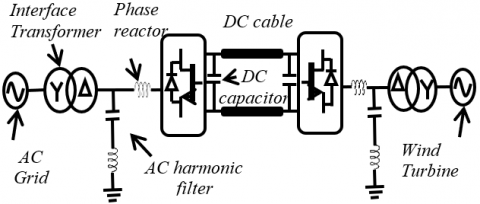
The VSC-HVDC scheme is shown in Figure 1. A DC cable is made as connection between the two VSC stations. On the DC side, capacitors permit to conserve the DC voltage and the phase reactors filter injected grid currents. On the AC side, the converter is connected to an AC network or a wind turbine with a transformer in order to insulate the station from the AC source and provides the appropriate AC voltage. The phase reactors associated with the transformer filter injected grid currents. Optional AC filters are exploited to supply the reactive power and also to filter Pulse-Width Modulation (PWM) harmonics.
Figure 1. VSC-HVDC transmission system
The various control methods developed in view of controlling the VSC-HVDC system can operate suitably in case of a communication failure. Specially the Master-Slave method and the Voltage Droop method [22]. The Voltage Droop method is typically used when more than one converter is controlling the DC voltage at the same time. On the other hand, the Master-Slave method is a simple control method adapted to command the VSC-HVDC system. Indeed, there is only one converter called Master one. It controls the DC bus voltage to keep it in a certain range. While the other converters which are called Slave, control their power by injecting or extracting the power to from the DC grid. For point to point HVDC structure the Master Slave control method is usually sufficient [22].
The dq rotating structure used for the modelling and controlling of an AC system is employed with the aim of attaining stationary electrical equations. To pathway the AC grid voltage frequency and the phase angle, a Phase Lock Loop (PLL) is applicated. In such a case, the q-axis voltage is null and the d-axis is synchronized with the grid voltage vector and has similar amplitude as the point of common coupling voltage vector. Thus, the active and reactive powers are separately controlled by current constituent [9].
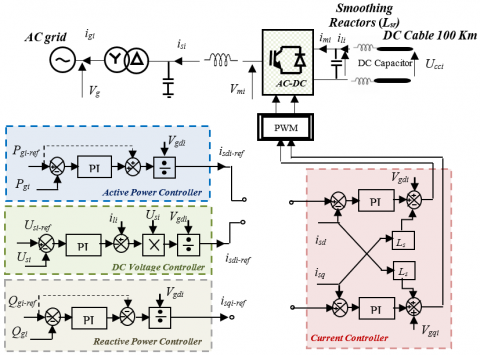
As shown in Figure 2 which presents a VSC substation controlled in dq synchronous frame, the control system is divided into two parts: the inner control loop is used to control the currents (isd and isq) by adjusting d and q coordinates of modulated voltages (Vmd and Vmq) in the Park frame, and the outer control loop is used to achieve precise functions: The d-axis current reference (isd-ref) can be generated by an active power or DC voltage controller. The q-axis current reference (isq-ref) can be obtained by a reactive power or AC voltage controller.
Figure 2. Point to-point controlled VSC-HVDC link
where:
Rs Ls: Resistance, Inductance of the phase reactors associated with the interface transformer filter.
Cs: DC capacitors.
Lsr: Smoothing reactors.
Lg Cg: Inductance, Capacitance of the AC filter.
(vgi, igi): The couple voltage-current of an AC grid.
(usi, ici): The couple voltage-current of the DC bus.
(vmdi-ref, vmqi-ref): Direct and quadrature control voltages of converter.
(vmi, imi): Couple voltage-current delivered by the converter.
(Pgi, Qgi): The active and reactive power through the system.
(Usi-ref): The DC Voltage reference.
(Pgi-ref, Qgi-ref): The reference active and reactive power delivered by the transformer.
(Pmi, Qmi): Active and reactive power delivered by the converter.
isi: The phase reactor current.
ili: The cable current.
uCci: The voltage cable.
The i index ϵ {1, 2}, it indicates the station number.
2.2 Stability study of the HVDC link via small signal stability method
2.2.1 Linearization of a VSC-HVDC link
The stability of a system is its capability, for an operating point to find equilibrium after a physical disturbance. Traditionally, the system stability is tested when it is submissive to small disturbance. Therefore, a linearized model of the system is created to analyse its stability [7-23]. In this part, we present a technique to model VSC-HVDC converter station for dynamic study.
In this work, the converter is deemed ideal and it is simulated by its average model in view of not taking into account harmonics effects [24], which are not our a matter of interest in this work. Indeed, the average-value model of the converter has the same dynamic performance of the detailed model, it is also more efficient for simulation time steps as explained in the study [25]. In this section, the linearization of the various components of a HVDC liaison is presented.
The general state space of a linearized system is expressed by [26]:
$\left\{\begin{array}{l}\Delta \dot{X}=A \Delta \dot{X}+B \Delta U \\ \Delta Y=C \Delta X+D \Delta U\end{array}\right.$ (1)
where, for each considered subsystem: ΔX is the state vector, ∆U is the input vector and the output vector is presented by ∆Y, A is the state matrix, the input matrix is B, the output matrix is presented by C, and the feed-forward matrix is presented by D.
We notice that the linearized block diagram of each subsystem presented in Figures 3, 4, 5 and 6 contains a proportional integral (PI) regulator. Therefore, to facilitate the creation of a global state space model, we choose to change the model defined by Eq. (1) to an increased one by adding a new state auxiliary vector "∆Z" to the main state vector "∆X" in order to eliminate the use of the controller [9]. Thus, the new state space system is obtained:
$\left\{ \begin{array}{l}\Delta \mathop {X'}\limits^. = A'\Delta \mathop {X'}\limits^. + B'\Delta U'\\\Delta Y' = C'\Delta X' + D'\Delta U'\end{array} \right.$ (2)
With $\Delta X' = \left[ \begin{array}{l}\Delta X\\\Delta Z\end{array} \right]$ (3)
where, ∆X’ is the new state vector, ∆U’ is the new input vector, the new output vector is presented by ∆Y’, A’ is the new state matrix, B’ is the new input matrix, new output matrix is given by C’ and finally, D’ is the new feed-forward matrix. However, when the state matrix A’ is. null, we fix the controlled state vector ∆U’ as: ∆U’=k∆X’. With: k is the gain matrix assuring the stability of the system.
A current controller linear model
The model of the VSC-HVDC system associated to its current control loop as given in Figure 2 is the basic structure for such VSC system connected to grid. Disregarding the switching losses, power at both sides of the converter is the same: Assumptions are made with the aim of simplifying the complexity of the system and making the AC side of the VSC not to impact the DC system. With this assumption and referring to Figure 2, we can assume that:
$V_{m d i} i_{s d i}+V_{m d i} i_{s q i}=U_{s i} i_{m i}=P_{m i}$ (4)
Eq. (4) is not linear. So, with the aim of evaluating its stability, we should linearize the system around an operating point. Each quantity is prescribed by an operating point denoted by capital letter and the subscript 0, and a small variation denoted by the Greek symbol. After linearization, Eq. (4) becomes:
$\Delta {V_{mdi}}{I_{sd0}} + \Delta {i_{sdi}}{V_{md0}} + \Delta {V_{mqi}}{I_{sq0}} + \Delta {i_{sqi}}{V_{mq0}} = \Delta {U_{si}}{I_{m0}} + \Delta {i_{mi}}{U_{s0}}$ (5)
The i index refers to the station number which is in this case ϵ{1, 2}.
Thus, the linearized current controller of a VSC is presented in Figure 3.
The steady state error between the reference and the output current ought to be avoided by the integration of a PI controller in the current controller. The corrector gain of the current controller PI corrector is defined by:
$P I=\frac{K_{p i} p+K_{i i}}{p}$ (6)
With: p presents Laplace Coefficient. The transfer function (TF) of the current control is the same for the two axes. The expression of the d-axis current control loop transfer function is expressed by:
$\frac{{{i_{sd}}}}{{{i_{sd - ref}}}}(p) = \frac{{1 + \frac{{{K_{pi}}}}{{{K_{ii}}}}p}}{{1 + \frac{{{K_{pi}} + {R_s}}}{{{K_{ii}}}}p + \frac{{{L_s}}}{{{K_{ii}}}}{p^2}}}$ (7)
The formulations of Kpi and Kii deduced from the pole placement method, are:
$K_{p v}=2 \zeta w_{n} C_{s}$ and $K_{i i}=L_{s} w_{n}^{2}$ (8)
where: $\zeta$ is the damping ratio.
$w_{n} \frac{3}{T_{r}}$ is the natural frequency [rad/s].
To create the new state space current controller, we choose new state variables $\Delta Z_{1 i}$ and $\Delta Z_{2 i}$ such as:
$\left\{ \begin{array}{l}\frac{{d(\Delta {Z_{1i}})}}{{dt}} = \Delta {i_{sdi - ref}} - \Delta {i_{sdi}}\\\frac{{d(\Delta {Z_{2i}})}}{{dt}} = \Delta {i_{sqi - ref}} - \Delta {i_{sqi}}\end{array} \right.$ (9)
The vectors and the following matrices represent the new linearized current controller state space representation according to the system (2).
$\Delta X^{\prime}=\left[\begin{array}{c}\Delta i_{s d i} \\ \Delta i_{s q i} \\ \Delta U_{s i} \\ \Delta Z_{1 i} \\ \Delta Z_{2 i}\end{array}\right] \Delta U^{\prime}=\left[\begin{array}{c}\Delta i_{s d i-r e f} \\ \Delta i_{s q i-r e f}\end{array}\right] ; \Delta Y^{\prime}=\left[\begin{array}{c}\Delta i_{s d i} \\ \Delta i_{s q i} \\ \Delta U_{s i}\end{array}\right]$ (10)
Figure 3. Linearized block diagram of the current controller VSC
$A' = \left[ {\begin{array}{*{20}{c}}{\frac{{ - {R_s}}}{{{L_s}}}}&0&0&{\frac{1}{{{L_s}}}}&0\\0&{\frac{{ - {R_s}}}{{{L_s}}}}&0&0&{\frac{1}{{{L_s}}}}\\{(\frac{{ - {V_{md0}} - {I_{sq0}}{L_s}w}}{{{C_s}{U_{s0}}}} +\frac{{z{'_1}}}{{{C_s}}})}&{(\frac{{ - {V_{mq0}} + {I_{sd0}}{L_s}w}}{{{C_s}{U_{s0}}}} + \frac{{z{'_2}}}{{{C_s}}})}&{(\frac{{{I_{m0}}}}{{{C_s}{U_{s0}}}} + \frac{{z{'_3}}}{{{C_s}}})}&{(\frac{{ - {I_{sd0}}}}{{{C_s}{U_{s0}}}} + \frac{{z{'_4}}}{{{C_s}}})}&{(\frac{{ - {I_{sq0}}}}{{{C_s}{U_{s0}}}} + \frac{{z{'_5}}}{{{C_s}}})}\\
{ - 1}&0&0&0&0\\0&{ - 1}&0&0&0\end{array}} \right]$
$B^{\prime}=\left[\begin{array}{ll}0 & 0 \\ 0 & 0 \\ 0 & 0 \\ 1 & 0 \\ 0 & 1\end{array}\right]$; $C^{\prime}=\left[\begin{array}{lllll}1 & 0 & 0 & 0 & 0 \\ 0 & 1 & 0 & 0 & 0 \\ 0 & 0 & 1 & 0 & 0\end{array}\right]$; $D^{\prime}=\left[\begin{array}{ll}0 & 0 \\ 0 & 0 \\ 0 & 0\end{array}\right]$ (11)
where, The i index ϵ {1, 2}, it means the station number and $Z_{1}^{\prime}, Z_{2}^{\prime}, Z_{3}^{\prime}, Z_{4}^{\prime},$ and $Z_{5}^{\prime}$, are constant values.
A Power controller Linear model
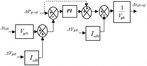
Figure 4. Linearized block diagram of the active power controller
The linearized model of the active power controller is illustrated in Figure 4.
After linearization, the expressions of the active power $P_{g i}$ and reactive power $Q_{g i}$ presented in Figure 2 become:
$\Delta P_{g i}=\Delta V_{g d i} I_{s d 0}+\Delta i_{s d i} V_{g d 0}$ (12)
$\Delta Q_{g i}=-\left(\Delta V_{g d i} I_{s q 0}+\Delta i_{s q i} V_{g d 0}\right)$ (13)
The PI power controller is expressed by:
$P I=\frac{K_{p p} p+K_{i p}}{p}$ (14)
The power control transfer function has the following form:
$\frac{{{P_g}}}{{{P_{g - ref}}}}(p) = \frac{{1 + \frac{{{K_{pp}}}}{{{K_{ip}}}}p}}{{1 + \frac{{1 + {K_{pp}}}}{{{K_{ip}}}}p}}$ (15)
This TF is assimilated at a first order TF with a time constant $\Gamma_{p}=\frac{T_{r}}{3}$. In order to reach a required response time, the parameters of the power controller are:
$K_{p p}=0$ and $K_{i p}=\frac{1}{\Gamma_{p}}$ (16)
According to the active power controller linearized block diagram defined in Figure 4, we define the new state variables “$\Delta Z_{a i}$” and “$\Delta Z_{r i}$” respectively related to the active and reactive power controller:
$\left\{ \begin{array}{l}\frac{{d\Delta {Z_{ai}}}}{{dt}} = \Delta {P_{gi - ref}} - \Delta {i_{sdi}}{V_{gd0}} - \Delta {V_{gdi}}{I_{sd0}}\\\frac{{d\Delta {Z_{ri}}}}{{dt}} = \Delta {Q_{gi - ref}} - \Delta {i_{sqi}}{V_{gd0}} - \Delta {V_{gdi}}{I_{sq0}}\end{array} \right.$ (17)
For the active power controller, we obtain:
$\Delta X^{\prime}=\left[\begin{array}{l}\Delta i_{\text {sdi-ref}} \\ \Delta Z_{a i}\end{array}\right] ; \Delta U^{\prime}=\left[\begin{array}{l}\Delta P_{\text {gi-ref}} \\ \Delta i_{\text {sdi}} \\ \Delta V_{\text {gdi}}\end{array}\right] ; \Delta Y^{\prime}=\Delta i_{\text {sdi-ref}}$ (18)
$A^{\prime}=\left[\begin{array}{ll}0 & 0 \\ 0 & 0\end{array}\right] ; B^{\prime}=\left[\begin{array}{ccc}0 & 0 & 0 \\ 1 & -V_{g d 0} & -I_{s d 0}\end{array}\right] ; \quad C^{\prime}=\left[\begin{array}{ll}0 & \frac{1}{V_{g d 0}}\end{array}\right]$ and $D^{\prime}=\left[\frac{1}{V_{g d 0}} 0-\frac{I_{s d 0}}{V_{g d 0}}\right]$ (19)
And for the reactive power controller, we obtain:
$\Delta X^{\prime}=\left[\begin{array}{c}\Delta i_{s q i-r e f} \\ \Delta Z_{r i}\end{array}\right] ; \Delta U^{\prime}=\left[\begin{array}{l}\Delta Q_{g i-r e f} \\ \Delta V_{g d i} \\ \Delta i_{s q i}\end{array}\right] ; \Delta Y^{\prime}=\Delta i_{s q i-r e f}$ (20)
$A^{\prime}=\left[\begin{array}{ll}0 & 0 \\ 0 & 0\end{array}\right] ; B^{\prime}=\left[\begin{array}{ccc}0 & 0 & 0 \\ 1 & I_{s q 0} & V_{g d 0}\end{array}\right] ; C^{\prime}=\left[\begin{array}{ll}0 & -\frac{1}{V_{g d 0}}\end{array}\right]$ and $D^{\prime}=\left[-\frac{1}{V_{g d 0}}-\frac{I_{s q 0}}{V_{g d 0}} 0\right]$ (21)
In this case the gain K defined in the respective feedback power controller, is fixed assuring the final form of the matrix A’1=N’K [27].
B. DC voltage controller Linear Model
The balance of powers proves that the DC power is converted to real power in the AC part when we neglect the phase reactor and the shunt conductance capacitance losses. Indeed, the conclusions of our analysis will be only due to the interaction between converter controllers and the DC grid. So the relation between AC and DC side can be written as follows:
${{i}_{m}}{{U}_{s}}={{P}_{g}}={{i}_{sd}}{{V}_{gd}}$ (22)
Thus, the linearization of the Eq. (22) is developed as follows:
${{I}_{m0}}\Delta {{U}_{si}}+{{U}_{s0}}\Delta {{i}_{mi}}={{I}_{sd0}}\Delta {{V}_{gdi}}+\Delta {{i}_{sdi-ref}}{{V}_{gd0}}$ (23)
The PI used in the DC voltage controller is expressed by:
$PI=\frac{{{K}_{pv}}p+{{K}_{iv}}}{p}$ (24)
The linearized model of the DC voltage controller is illustrated in Figure 5.
Figure 5. Block diagram of the linearized DC voltage controller
The voltage control loop transfer function is:
$\frac{{{U}_{si}}}{{{U}_{si-ref}}}(p)=\frac{1}{1+\frac{{{K}_{pv}}}{{{K}_{iv}}}p+\frac{{{C}_{s}}}{{{K}_{iv}}}{{p}^{2}}}$ (25)
The parameters of the controller are deduced by identifying the polynomial characteristic of the voltage TF to the desired second order polynomial.
${{K}_{iv}}={{C}_{s}}w_{n}^{2}$and${{K}_{pv}}=2\zeta {{w}_{n}}{{C}_{s}}$ (26)
where, $\zeta$ is the damping ratio and wn is the natural frequency.
In accordance with the linearized block diagram of the voltage controller defined in Figure 5, a new state variable “$\Delta Z_{v i}$” ought to be created.
where,
$\frac{d\Delta {{Z}_{vi}}}{dt}=\Delta {{U}_{si-ref}}-\Delta {{U}_{si}}$ (27)
Thus, we obtain:
$\Delta X^{\prime}=\left[\begin{array}{l}\Delta i_{\text {sdi-ref}} \\ \Delta Z_{v i}\end{array}\right]$;
$\Delta {{U}^{'}}=\left[ \begin{align} & \Delta \mathop{U}_{si-ref} \\ & \Delta \mathop{V}_{vgdi} \\ & \Delta \mathop{U}_{si} \\ & \Delta \mathop{i}_{li} \\\end{align} \right]$; (28)
$\Delta Y^{\prime}=\Delta i_{\text {sdi-ref}}$
$A^{\prime}=\left[\begin{array}{ll}0 & 0 \\ 0 & 0\end{array}\right] ; B^{\prime}=\left[\begin{array}{llll}0 & 0 & 0 & 0 \\ 1 & 0 & -1 & 0\end{array}\right] ; C^{\prime}=\left[\begin{array}{ll}0 & -\frac{U_{s 0}}{V_{g d 0}}\end{array}\right]$ and $D^{\prime}=\left[\begin{array}{llll}0 & -\frac{I_{s d 0}}{V_{g d 0}} & \frac{I_{m 0}}{V_{g d 0}} & \frac{U_{s 0}}{V_{g d 0}}\end{array}\right]$ (29)
2.2.2 Studied VSC-HVDC model association
To find a liaison between two subsystems which are constituents of a total system ⅀, two systems ⅀A and ⅀B are designed.
The index 'a' is an auxiliary subscribe identifying ⅀A. The state space model of ⅀A is defined by:
$\Sigma A=\left\{\begin{array}{l}\frac{d}{d t}\left[\begin{array}{l}X_{a 1} \\ X_{a 2}\end{array}\right]=A_{a}\left[\begin{array}{l}X_{a 1} \\ X_{a 2}\end{array}\right]+B_{a}\left[\begin{array}{l}U_{a 1} \\ U_{a 2}\end{array}\right] \\ {\left[\begin{array}{l}Y_{a 1} \\ Y_{a 2}\end{array}\right]=C_{a}\left[\begin{array}{l}X_{a 1} \\ X_{a 2}\end{array}\right]+D_{a}\left[\begin{array}{l}U_{a 1} \\ U_{a 2}\end{array}\right]}\end{array}\right.$ (30)
The index 'b' is an auxiliary subscribe identifying ⅀B. The state space representation of ⅀B is defined by:
$\Sigma B=\left\{\begin{array}{l}\frac{d}{d t}\left[\begin{array}{l}X_{b 1} \\ X_{b 2}\end{array}\right]=A_{b}\left[\begin{array}{l}X_{b 1} \\ X_{b 2}\end{array}\right]+B_{a}\left[\begin{array}{l}U_{b 1} \\ U_{b 2}\end{array}\right] \\ {\left[\begin{array}{l}Y_{b 1} \\ Y_{b 2}\end{array}\right]=C_{b}\left[\begin{array}{l}X_{b 1} \\ X_{b 2}\end{array}\right]+D_{b}\left[\begin{array}{l}U_{b 1} \\ U_{b 2}\end{array}\right]}\end{array}\right.$ (31)
In the whole system, the transfer matrix $T_{a b}$ links the inputs of subsystem $\sum A$ to the outputs of subsystem $\sum B$ :
$\left[\begin{array}{l}U_{a 1} \\ U_{a 2}\end{array}\right]=T_{a b}\left[\begin{array}{l}Y_{b 1} \\ Y_{b 2}\end{array}\right]$ (32)
In the same manner, the transfer matrix $T_{b a}$ links the inputs of subsystem $\sum B$ to the outputs of subsystem $\sum A,$ in the global system:
$\left[\begin{array}{l}U_{b 1} \\ U_{b 2}\end{array}\right]=T_{b a}\left[\begin{array}{l}Y_{a 1} \\ Y_{a 2}\end{array}\right]$ (33)
Hence, the state space representation of the global system is:
$\Sigma=\left\{\begin{array}{l}\frac{d}{d t}\left[\begin{array}{l}X_{a 1} \\ X_{a 2} \\ X_{b 1} \\ X_{b 2}\end{array}\right]=A\left[\begin{array}{l}X_{a 1} \\ X_{a 2} \\ X_{b 1} \\ X_{b 2}\end{array}\right]+B\left[\begin{array}{l}U_{a 1} \\ U_{a 2} \\ U_{b 1} \\ U_{b 2}\end{array}\right] \\ {\left[\begin{array}{l}Y_{a 1} \\ Y_{a 2} \\ Y_{b 1} \\ Y_{b 2}\end{array}\right]=C\left[\begin{array}{l}X_{a 1} \\ X_{a 2} \\ X_{b 1} \\ X_{b 2}\end{array}\right]+D\left[\begin{array}{l}U_{a 1} \\ U_{a 2} \\ U_{b 1} \\ U_{b 2}\end{array}\right]}\end{array}\right.$ (34)
Presuming that the state variables of the total system are a juxtaposition of subsystems state variables in order to build the system ⅀ based to [28]. As well, a combination of subsystem inputs constitutes the inputs of the total system. To retrieve the state variables of subsystems within the total system, subsystems are arranged in the order in the total system.
The form of the state space matrices A, B, C and D of the global system which are resulted from the associations of state space matrices of each subsystem are defined by [28]:
$A=\left[\begin{array}{cc}A_{1} & B_{1} T_{12} C_{2} \\ B_{2} T_{21} C_{1} & A_{2}\end{array}\right] B=\left[\begin{array}{cc}{[0]} & B_{1} T_{12} D_{2} \\ B_{2} T_{21} D_{1} & {[0]}\end{array}\right]$
$C=\left[ \begin{matrix} \mathop{C}_{1} & \left[ 0 \right] \\ \left[ 0 \right] & \mathop{C}_{2} \\\end{matrix} \right]$; $D=\left[ \begin{matrix} \mathop{D}_{1} & \left[ 0 \right] \\ \left[ 0 \right] & \mathop{D}_{2} \\\end{matrix} \right]$ (35)
A. State space model of station1
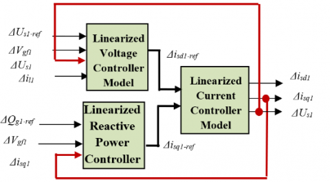
In order to find the state space model of station1, we studied the link between the state space model of the voltage controller and the state space model of the active power controller with the state space model of the current controller as presented in Figure 6.
First, a development of the state space model of the voltage controller with the state space model of the reactive power controller is done. The reached model is deduced directly from the state space model of each subsystem, so, we obtain:
$\left\{\begin{array}{l}\mathrm{\frac{d}{d t}\left[\begin{array}{l}\Delta i_{s d 1-r e f} \\ \Delta Z_{v} \\ \Delta i_{s q 1-r e f} \\ \Delta Z_{r 1}\end{array}\right]=\left[\begin{array}{cccc}0 & 0 & 0 & 0 \\ p_{5} & p_{6} & 0 & 0 \\ 0 & 0 & 0 & 0 \\ 0 & 0 & p_{3} & p_{4}\end{array}\right]\left[\begin{array}{l}\Delta i_{s d 1-r e f} \\ \Delta Z_{v} \\ \Delta i_{s q 1-r e f} \\ \Delta Z_{r 1}\end{array}\right]+\left[\begin{array}{cccccc}0 & 0 & 0 & 0 & 0 & 0 \\ 1 & 0 & -1 & 0 & 0 & 0 \\ 0 & 0 & 0 & 0 & 0 & 0 \\ 0 & I_{s q 0} & 0 & 0 & 1 & V_{g d 0}\end{array}\right]\left[\begin{array}{l}\Delta U_{s 1-r e f} \\ \Delta V_{g d 1} \\ \Delta U_{s 1} \\ \Delta i_{l 1} \\ \Delta Q_{g 1-r e f} \\ \Delta U_{i s q 1}\end{array}\right]} \\ \mathrm{\frac{d}{d t}\left[\begin{array}{c}i_{s d 1-r e f} \\ i_{s q 1-r e f}\end{array}\right]=\left[\begin{array}{cccc}0 & -\frac{U_{s 0}}{V_{g d}} & 0 & 0 \\ 0 & 0 & 0 & -\frac{1}{V_{g d 0}}\end{array}\right]\left[\begin{array}{l}\Delta i_{s d 1-r e f} \\ \Delta Z_{v} \\ \Delta i_{s q 1-r e f} \\ \Delta Z_{r 1}\end{array}\right]+\left[\begin{array}{cccccc}0 & -\frac{I_{s d 0}}{V_{g d 0}} & \frac{I_{m 0}}{V_{g d 0}} & \frac{U_{s 0}}{V_{g d 0}} & 0 & 0 \\ 0 & -\frac{I_{s q 0}}{V_{g d 0}} & 0 & 0 & -\frac{1}{V_{g d 0}} & 0\end{array}\right]\left[\begin{array}{l}\Delta U_{s 1-r e f} \\ \Delta V_{g d 1} \\ \Delta U_{s 1} \\ \Delta i_{l 1} \\ \Delta Q_{g 1-r e f} \\ \Delta U_{i s q 1}\end{array}\right]}\end{array}\right.$ (36)
where, $p_{j} ; j \in\{3,4,5,6\}$ is a constant value, representing the elements of the state matrix of the system (36).
Figure 6. Global model of station1
Then, to have the state space model of station1, we determined the transfer matrix $T_{a b 1}$ between the inputs of subsystem obtained by the voltage and reactive power controllers’ models connected together and the output of the current controller model. This matrix is defined as:
$T_{a b 1}=\left[\begin{array}{l}\Delta U_{s 1-r e f} \\ \Delta V_{g d 1} \\ \Delta U_{s 1} \\ \Delta i_{l 1} \\ \Delta Q_{g 1-r e f} \\ \Delta i_{s q 1}\end{array}\right]=\left[\begin{array}{lll}0 & 0 & 0 \\ 0 & 0 & 0 \\ 0 & 0 & 1 \\ 0 & 0 & 0 \\ 0 & 0 & 0 \\ 0 & 1 & 0\end{array}\right]\left[\begin{array}{l}\Delta i_{s d 1} \\ \Delta i_{s q 1} \\ \Delta U_{s 1}\end{array}\right]$ (37)
The transfer matrix $T_{a b 1}$ given in Eq. (38), links the inputs of the voltage controller model with the reactive power controller model and the output of the current controller model.
$T_{b a 1}=\left[\begin{array}{c}\Delta i_{s d 1-r e f} \\ \Delta i_{s q 1-r e f}\end{array}\right]=\left[\begin{array}{cc}1 & 0 \\ 0 & 1\end{array}\right]\left[\begin{array}{l}\Delta i_{s d 1-r e f} \\ \Delta i_{s q 1-r e f}\end{array}\right]$ (38)
So, we deduced the global state space model of station1, as given in system (39):
$\left\{\begin{array}{l}\mathrm{\frac{d}{d t}\left[\begin{array}{l}\Delta i_{s d 1-r e f} \\ \Delta Z_{v} \\ \Delta i_{s q 1-r e f} \\ \Delta Z_{r 1} \\ \Delta i_{s d 1} \\ \Delta i_{s q 1} \\ \Delta U_{s 1} \\ \Delta Z_{11} \\ \Delta Z_{21}\end{array}\right]=\left[\begin{array}{ccccccccc}0 & 0 & 0 & 0 & 0 & 0 & 0 & 0 & 0 \\ p_{5} & p_{6} & 0 & 0 & 0 & 0 & -1 & 0 & 0 \\ 0 & 0 & 0 & 0 & 0 & 0 & 0 & 0 & 0 \\ 0 & 0 & p_{3} & p_{4} & 0 & V_{g d 0} & 0 & 0 & 0 \\ 0 & 0 & 0 & 0 & \frac{-R_{s}}{L_{s}} & 0 & 0 & \frac{1}{L_{s}} & 0 \\ 0 & 0 & 0 & 0 & 0 & \frac{-R_{s}}{L_{s}} & 0 & 0 & \frac{1}{L_{s}} \\ 0 & 0 & 0 & 0 & a_{1} & a_{2} & a_{3} & a_{4} & a_{5} \\ 0 & \frac{-U_{s 0}}{V_{g d 0}} & 0 & 0 & & 0 & 0 & 0 & 0 \\ 0 & 0 & 0 & \frac{-1}{V_{g d}} & 0 & -1 & 0 & 0 & 0\end{array}\right]\left[\begin{array}{l}\Delta i_{s d 1-r e f} \\ \Delta Z_{v} \\ \Delta i_{s q 1-r e f} \\ \Delta Z_{r 1} \\ \Delta i_{s d 1} \\ \Delta i_{s q 1} \\ \Delta U_{s 1} \\ \Delta Z_{11} \\ \Delta Z_{21}\end{array}\right]+\left[\begin{array}{cccccccc}0 & 0 & 0 & 0 & 0 & 0 & 0 & 0 \\ 0 & 0 & 0 & 0 & 0 & 0 & 0 & 0 \\ 0 & 0 & 0 & 0 & 0 & 0 & 0 & 0 \\ 0 & 0 & 0 & 0 & 0 & 0 & 0 & 0 \\ 0 & 0 & 0 & 0 & 0 & 0 & 0 & 0 \\ 0 & 0 & 0 & 0 & 0 & 0 & 0 & 0 \\ 0 & \frac{-I_{s d 0}}{V_{g d 0}} & \frac{-I_{m 0}}{V_{g d 0}} & \frac{-U_{s 0}}{V_{g d 0}} & 0 & 0 & 0 & 0 \\ 0 & \frac{-I_{s q 0}}{V_{g d 0}} & 0 & 0 & \frac{-1}{V_{g d 0}} & 0 & 0 & 0\end{array}\right]\left[\begin{array}{l}\Delta U_{s 1-r e f} \\ \Delta V_{g d 1} \\ \Delta U_{s 1} \\ \Delta i_{l 1} \\ \Delta Q_{g 1-r e f} \\ \Delta i_{s q 1} \\ \Delta i_{s d 1-r e f} \\ \Delta i_{s q 1-r e f}\end{array}\right]} \\ \mathrm{\left[\begin{array}{l}\Delta i_{\text {sd1-ref}} \\ \Delta i_{\text {sq1-ref}} \\ \Delta i_{s d 1} \\ \Delta i_{\text {sq1}}\end{array}\right]=\left[\begin{array}{ccccccccc}0 & \frac{-U_{s 0}}{V_{g d 0}} & 0 & 0 & 0 & 0 & 0 & 0 & 0 \\ 0 & 0 & 0 & \frac{-1}{V_{g d 0}} & 0 & 0 & 0 & 0 & 0 \\ 0 & 0 & 0 & 0 & 1 & 0 & 0 & 0 & 0 \\ 0 & 0 & 0 & 0 & 0 & 1 & 0 & 0 & 0 \\ 0 & 0 & 0 & 0 & 0 & 0 & 1 & 0 & 0\end{array}\right]\left[\begin{array}{l}\Delta i_{\text {sd1-ref}} \\ \Delta Z_{v} \\ \Delta i_{\text {sq1-ref}} \\ \Delta Z_{r 1} \\ \Delta i_{\text {sd} 1} \\ \Delta i_{\text {sq} 1} \\ \Delta U_{s 1} \\ \Delta Z_{11} \\ \Delta Z_{21}\end{array}\right]+\left[\begin{array}{cccccccc}0 & \frac{-I_{s d 0}}{V_{g d 0}} & \frac{I_{m 0}}{V_{g d 0}} & \frac{U_{s 0}}{V_{g d 0}} & 0 & 0 & 0 & 0 \\ 0 & \frac{-I_{s q 0}}{V_{g d 0}} & 0 & 0 & \frac{-1}{V_{g d 0}} & 0 & 0 & 0 \\ 0 & 0 & 0 & 0 & 0 & 0 & 0 & 0 \\ 0 & 0 & 0 & 0 & 0 & 0 & 0 & 0 \\ 0 & 0 & 0 & 0 & 0 & 0 & 0 & 0\end{array}\right]\left[\begin{array}{l}\Delta U_{s 1-r e f} \\ \Delta V_{g d 1} \\ \Delta U_{s 1} \\ \Delta i_{l 1} \\ \Delta Q_{g 1-r e f} \\ \Delta i_{s q 1} \\ \Delta i_{s d 1-r e f} \\ \Delta i_{s q 1-r e f}\end{array}\right]}\end{array}\right.$ (39)
$\left\{\begin{array}{l}\mathrm{\frac{d}{d t}\left\lfloor\begin{array}{l}\Delta i_{s d 2-r e f} \\ \Delta Z_{a} \\ \Delta i_{s q 2-r e f} \\ \Delta Z_{r 2}\end{array}\right]=\left[\begin{array}{cccc||c}0 & 0 & 0 & 0 \\ p_{1} & p_{2} & 0 & 0 \\ 0 & 0 & 0 & 0 \\ 0 & 0 & p_{3} & p_{4}\end{array}\right]\left[\begin{array}{l}\Delta i_{s d 2-r e f} \\ \Delta Z_{a} \\ \Delta i_{s q 2-r e f} \\ \Delta Z_{r 2}\end{array}\right]+\left[\begin{array}{ccccc}0 & 0 & 0 & 0 & 0 \\ 1 & -V_{g d 0} & -I_{s d 0} & 0 & 0 \\ 0 & 0 & 0 & 0 & 0 \\ 0 & 0 & I_{s q 0} & 1 & V_{g d 0}\end{array}\right]\left[\begin{array}{l}\Delta P_{g 2-r e f} \\ \Delta i_{s d 2} \\ \Delta V_{g d 2} \\ \Delta Q_{g 2-r e f} \\ \Delta i_{s q 2}\end{array}\right]} \\ \mathrm{\left[\begin{array}{c}\Delta i_{s d 1-r e f} \\ \Delta i_{s q 1-r e f}\end{array}\right]=\left[\begin{array}{cccc}0 & \frac{1}{V_{g d 0}} & 0 & 0 \\ 0 & 0 & 0 & \frac{-1}{V_{g d 0}}\end{array}\right]\left[\begin{array}{l}\Delta i_{s d 2-r e f} \\ \Delta Z_{a} \\ \Delta i_{s q 2-r e f} \\ \Delta Z_{r 2}\end{array}\right]+\left[\begin{array}{ccccc}\frac{1}{V_{g d 0}} & 0 & \frac{-I_{s d 0}}{V_{g d 0}} & 0 & 0 \\ 0 & 0 & \frac{-I_{s q 0}}{V_{g d 0}} & \frac{-1}{V_{g d 0}} & 0\end{array}\right]\left[\begin{array}{l}\Delta P_{g 2-r e f} \\ \Delta i_{s d 2} \\ \Delta V_{g d 2} \\ \Delta Q_{g 2-r e f} \\ \Delta i_{s q 2}\end{array}\right]}\end{array}\right.$ (40)
B. State Space model of station2
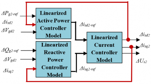
In the same way, we determined the state space model of station2, as presented in Figure 7. This station is controlled by the following controllers: active power, reactive power, and current controller.
Figure 7. Model of station2
First, a development of the state space model of the active power controller with the state space model of the reactive power controller is done. The reached model is deduced directly from the state space model of each subsystem, so, we obtain:
$p_{j} ; j \in\{1,2,3,4\}$ is a constant value, representing the elements of the state matrix of the system (40).
Then, in order to get the state space model of station2, we should determine the transfer matrix Tab2 between the inputs of subsystem obtained by the active and reactive power controllers’ models connected together and the output of the current controller model. This matrix is defined as:
$T_{a b 2}=\left[\begin{array}{l}\Delta P_{g 2-r e f} \\ \Delta i_{s d 2} \\ \Delta V_{g d 2} \\ \Delta Q_{g 2-r e f} \\ \Delta i_{s q 2}\end{array}\right]=\left[\begin{array}{lll}0 & 0 & 0 \\ 1 & 0 & 0 \\ 0 & 0 & 0 \\ 0 & 0 & 0 \\ 0 & 1 & 0\end{array}\right]\left[\begin{array}{l}\Delta i_{s d 2} \\ \Delta i_{s q 2} \\ \Delta U_{s 2}\end{array}\right]$ (41)
The transfer matrix Tab2 given in Eq. (42), links the inputs of the active power controller model with the reactive power controller model and the output of the current controller model.
$T_{b a 2}=\left[\begin{array}{l}\Delta i_{s d 2-\text {ref}} \\ \Delta i_{s q 2-r e f}\end{array}\right]=\left[\begin{array}{ll}1 & 0 \\ 0 & 1\end{array}\right]\left[\begin{array}{l}\Delta i_{s d 2-r e f} \\ \Delta i_{s q 2-r e f}\end{array}\right]$ (42)
So we deduced the state space model of station2:
$\left\{\begin{array}{l}\mathrm{\frac{d}{d t}\left[\begin{array}{l}\Delta i_{s d 2-r e f} \\ \Delta Z_{a} \\ \Delta i_{s q 2-r e f} \\ \Delta Z_{r 2} \\ \Delta i_{s d 2} \\ \Delta i_{s q 2} \\ \Delta U_{s 2} \\ \Delta Z_{12} \\ \Delta Z_{22}\end{array}\right]=\left[\begin{array}{ccccccccc}0 & 0 & 0 & 0 & 0 & 0 & 0 & 0 & 0 \\ p_{1} & p_{2} & 0 & 0 & -V_{g d 0} & 0 & 0 & 0 & 0 \\ 0 & 0 & 0 & 0 & 0 & 0 & 0 & 0 & 0 \\ 0 & 0 & p_{3} & p_{4} & 0 & V_{g d 0} & 0 & 0 & 0 \\ 0 & 0 & 0 & 0 & \frac{-R_{s}}{L_{s}} & 0 & 0 & \frac{1}{L_{s}} & 0 \\ 0 & 0 & 0 & 0 & 0 & \frac{-R_{s}}{L_{s}} & 0 & 0 & \frac{1}{L_{s}} \\ 0 & 0 & 0 & 0 & a_{1} & a_{2} & a_{3} & a_{4} & a_{5} \\ 0 & \frac{-1}{V_{g d 0}} & 0 & 0 & -1 & 0 & 0 & 0 & 0 \\ 0 & 0 & 0 & \frac{-1}{V_{g d 0}} & 0 & -1 & 0 & 0 & 0\end{array}\right]\left[\begin{array}{l}\Delta i_{s d 2-r e f} \\ \Delta Z_{a} \\ \Delta i_{s q 2-r e f} \\ \Delta Z_{r 2} \\ \Delta i_{s d 2} \\ \Delta i_{s q 2} \\ \Delta U_{s 2} \\ \Delta Z_{12} \\ \Delta Z_{22}\end{array}\right]+\left[\begin{array}{cccccccc}0 & 0 & 0 & 0 & 0 & 0 & 0 & 0 \\ 0 & 0 & 0 & 0 & 0 & 0 & 0 & 0 \\ 0 & 0 & 0 & 0 & 0 & 0 & 0 & 0 \\ 0 & 0 & 0 & 0 & 0 & 0 & 0 & 0 \\ 0 & 0 & 0 & 0 & 0 & 0 & 0 & 0 \\ 0 & 0 & 0 & 0 & 0 & 0 & 0 & 0 \\ 0 & \frac{-I_{s d 0}}{V_{g d 0}} & \frac{I_{m 0}}{V_{g d 0}} & \frac{I_{s d 0}}{V_{g d 0}} & 0 & 0 & 0 & 0 \\ 0 & \frac{-I_{s q 0}}{V_{g d 0}} & 0 & 0 & \frac{-1}{V_{g d 0}} & 0 & 0 & 0\end{array}\right]\left[\begin{array}{l}\Delta P_{g 2-r e f} \\ \Delta i_{s d 2} \\ \Delta V_{g d 2} \\ \Delta Q_{g 2-r e f} \\ \Delta i_{s q 2} \\ \Delta i_{s d 2-r e f} \\ \Delta i_{s q 2-r e f}\end{array}\right]} \\ \mathrm{\left[\begin{array}{l}\Delta i_{s d 2-r e f} \\ \Delta i_{s q 2-r e f} \\ \Delta i_{s d 2} \\ \Delta i_{s q 2} \\ \Delta U_{s 2}\end{array}\right]=\left[\begin{array}{ccccccccc}0 & \frac{1}{V_{g d 0}} & 0 & 0 & 0 & 0 & 0 & 0 & 0 \\ 0 & 0 & 0 & \frac{-1}{V_{g d 0}} & 0 & 0 & 0 & 0 & 0 \\ 0 & 0 & 0 & 0 & 1 & 0 & 0 & 0 & 0 \\ 0 & 0 & 0 & 0 & 0 & 1 & 0 & 0 & 0 \\ 0 & 0 & 0 & 0 & 0 & 0 & 1 & 0 & 0\end{array}\right]\left[\begin{array}{l}\Delta i_{s d 2-r e f} \\ \Delta Z_{a} \\ \Delta i_{s q 2-r e f} \\ \Delta Z_{r 2} \\ \Delta i_{s d 2} \\ \Delta i_{s q 2} \\ \Delta U_{s 2} \\ \Delta Z_{12} \\ \Delta Z_{22}\end{array}\right]+\left[\begin{array}{cccccccc}0 & \frac{-I_{s d 0}}{V_{g d 0}} & \frac{I_{m 0}}{V_{g d 0}} & \frac{U_{s 0}}{V_{g d 0}} & 0 & 0 & 0 & 0 \\ 0 & \frac{-I_{s q 0}}{V_{g d 0}} & 0 & 0 & \frac{-1}{V_{g d 0}} & 0 & 0 & 0 \\ 0 & 0 & 0 & 0 & 0 & 0 & 0 & 0 \\ 0 & 0 & 0 & 0 & 0 & 0 & 0 & 0 \\ 0 & 0 & 0 & 0 & 0 & 0 & 0 & 0\end{array}\right]\left[\begin{array}{l}\Delta P_{g 2-r e f} \\ \Delta i_{s d 2} \\ \Delta V_{g d 2} \\ \Delta Q_{g 2-r e f} \\ \Delta i_{s q 2} \\ \Delta i_{s d 2-r e f} \\ \Delta i_{s q 2-r e f}\end{array}\right]}\end{array}\right.$ (43)
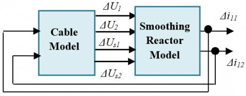
C. State Space model of system reactor and cable
The connection between the improved cable model and the smoothing reactor system model is illustrated in Figure 8.
Figure 8. Connection of the cable to the smoothing reactor
To determine the state space model of this association, we determined the transfer matrix Tab3 between the inputs of subsystem built from cable model and the output of the smoothing reactor model. This matrix is defined as:
$T_{a b 3}\left[\begin{array}{c}\Delta U_{s 1} \\ \Delta U_{c c 1} \\ \Delta U_{s 2} \\ \Delta U_{c c 2}\end{array}\right]=\left[\begin{array}{cc}0 & 0 \\ \frac{1}{2} & 0 \\ 0 & 0 \\ 0 & \frac{1}{2}\end{array}\right]\left[\begin{array}{c}\Delta U_{1} \\ \Delta U_{2}\end{array}\right]$ (44)
where, $U_{c c i}=\frac{U_{i}}{2}$
The transfer matrix Tab3 given in Eq. (45), links the inputs of the cable model and the output of the smoothing reactor model is defined by:
$T_{b a 3}\left[\begin{array}{c}\Delta i_{l 1} \\ \Delta i_{l 2}\end{array}\right]=\left[\begin{array}{ll}1 & 0 \\ 0 & 1\end{array}\right]\left[\begin{array}{l}\Delta i_{l 1} \\ \Delta i_{l 2}\end{array}\right]$ (45)
Thus, we obtained the state space model of the reactor, cable system association:
$\left\{\begin{array}{l}\mathrm{\frac{d}{d t}\left[\begin{array}{l}\Delta i_{l 1} \\ \Delta i_{l 2} \\ \Delta U_{c c 1} \\ \Delta U_{c c 2} \\ \Delta i_{L c 1} \\ \Delta i_{L c 2}\end{array}\right]=\left[\begin{array}{cccccc}p_{7} & p_{8} & \frac{1}{L_{s r}} & 0 & 0 & 0 \\ p_{9} & p_{10} & 0 & \frac{1}{L_{s r}} & 0 & 0 \\ \frac{-1}{C_{s}} & 0 & \frac{-G_{c}}{C_{c}} & 0 & \frac{-1}{C_{c}} & 0 \\ 0 & \frac{-1}{C_{c}} & 0 & \frac{-G_{c}}{C_{c}} & \frac{1}{C_{c}} & 0 \\ 0 & 0 & \frac{L_{c 2}}{L_{c 1} L_{c 2}-M_{c 12}^{2}} & \frac{-L_{c 2}}{L_{c 1} L_{c 2}-M_{c 12}^{2}} & \frac{-R_{c 1} L_{c 2}}{L_{c 1} L_{c 2}-M_{c 12}^{2}} & \frac{R_{c 1} M_{c 12}}{L_{c 1} L_{c 2}-M_{c 12}} \\ 0 & 0 & \frac{-M_{c 12}}{L_{c 1} L_{c 2}-M_{c 12}^{2}} & \frac{M_{c 12}}{L_{c 1} L_{c 2}-M_{c 12}^{2}} & \frac{R_{c 1} M_{c 12}}{L_{c 1} L_{c 2}-M_{c 12}^{2}} & \frac{-R_{c 2} L_{c 1}}{L_{c 1} L_{c 2}-M_{c 12}}\end{array}\right]\left[\begin{array}{l}\Delta i_{l 1} \\ \Delta i_{l 2} \\ \Delta U_{c c 1} \\ \Delta U_{c c 2} \\ \Delta i_{L c 1} \\ \Delta i_{L c 2}\end{array}\right]} \\ \mathrm{\left[\begin{array}{c}\Delta i_{l 1} \\ \Delta i_{l 2} \\ \Delta U_{1} \\ \Delta U_{2}\end{array}\right]=\left[\begin{array}{llllll}1 & 0 & 0 & 0 & 0 & 0 \\ 0 & 1 & 0 & 0 & 0 & 0 \\ 0 & 0 & 2 & 0 & 0 & 0 \\ 0 & 0 & 0 & 2 & 0 & 0\end{array}\right]\left[\begin{array}{c}\Delta i_{l 1} \\ \Delta i_{l 2} \\ \Delta U_{c c 1} \\ \Delta U_{c c 2} \\ \Delta i_{L c 1} \\ \Delta i_{L c 2}\end{array}\right]}\end{array}\right.$ (46)
where, $p_{j} ; j \in\{7,8,9,10\}$ is a constant value, representing some elements of the state matrix of the system (46).
D. State space model of the studied VSC-HVDC system
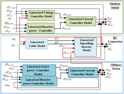
In the preceding parts, each linearized subsystem of the VSC-HVDC liaison is modeled as a linear state space model. With the aim of getting a total closed-loop model of the VSC-HVDC system, inputs and outputs of subsystems are linked together as shown in Figure 9.
After developing the link between the systems composed of station 1, station 2 and the system smoothing reactor with cable, we obtain the final state matrix A of the VSC-HVDC
System. As well, the final state vector ∆X', the final input vector ∆U' and the final output vector ∆Y' of the VSC-HVDC system are given as:
$\begin{align} & {{X}_{VSC-HVDC}}=\left[ \begin{matrix} \Delta {{i}_{sd1-ref}} & \Delta {{Z}_{v}} & \Delta {{i}_{sq1-ref}} & \Delta {{Z}_{r1}} & \Delta {{i}_{sd1}} & \Delta {{i}_{sq1}} & \Delta {{U}_{s1}} & \Delta {{Z}_{11}} & \Delta {{Z}_{21}} & \Delta {{i}_{sd2-ref}} & \Delta {{Z}_{a}} & \Delta {{i}_{sq2-ref}} \\\end{matrix} \right. \\ & {{\left. \begin{matrix} \Delta {{Z}_{r2}} & \Delta {{i}_{sd2}} & \Delta {{i}_{sq2}} & \Delta {{U}_{s2}} & \Delta {{Z}_{12}} & \Delta {{Z}_{22}} & \Delta {{i}_{l1}} & \Delta {{i}_{l2}} & \Delta {{U}_{cc1}} & \Delta {{U}_{cc2}} & \Delta {{i}_{Lc1}} & \Delta {{i}_{Lc2}} \\\end{matrix} \right]}^{T}} \\\end{align}$ (47)
$\begin{align} & \mathop{Y}_{VSC-HVDC}=\left[ \begin{matrix} \mathop{\Delta i}_{sd1-ref} & \mathop{\Delta i}_{sq1-ref} & \mathop{\Delta i}_{sd1} & \mathop{\Delta i}_{sq1} & \mathop{\Delta U}_{s1} & \mathop{\Delta i}_{sd2-ref} & \mathop{\Delta i}_{sq2-ref} & \mathop{\Delta i}_{sd2} & \mathop{\Delta i}_{sq2} & \mathop{\Delta U}_{s2} & \mathop{\Delta i}_{l1} & \mathop{\Delta i}_{l2} \\\end{matrix} \right. \\ & {{\begin{matrix} \mathop{\Delta U}_{1} & \left. \mathop{\Delta U}_{2} \right] \\\end{matrix}}^{T}} \\\end{align}$ (48)
$\begin{align} & {{U}_{VSC-HVDC}}=\left[ \begin{matrix} \Delta {{U}_{s1-ref}} & \Delta {{V}_{gd1}} & \Delta {{U}_{s1}} & \Delta {{i}_{l1}} & \Delta {{Q}_{g1-ref}} & \Delta {{i}_{sq1}} & \Delta {{i}_{sd1-ref}} & \Delta {{i}_{sq1-ref}} & \Delta {{P}_{g2-ref}} & \Delta {{i}_{sd2}} & \Delta {{V}_{gd2}} & \Delta {{Q}_{g2-ref}} \\\end{matrix} \right. \\ & {{\left. \begin{matrix} \Delta {{i}_{sq2}} & \Delta {{i}_{sd2-ref}} & \Delta {{i}_{sq2-ref}} & \Delta {{i}_{l1}} & \Delta {{i}_{l2}} & \Delta {{U}_{cc1}} & \Delta {{U}_{cc2}} \\\end{matrix} \right]}^{T}} \\\end{align}$ (49)
$A{}_{VSC-HVDC}=\left[ \begin{matrix} 0 & 0 & 0 & 0 & 0 & 0 & 0 & 0 & 0 & 0 & 0 & 0 & 0 & 0 & 0 & 0 & 0 & 0 & 0 & 0 & 0 & 0 & 0 & 0 \\ {{p}_{5}} & {{p}_{6}} & 0 & 0 & 0 & 0 & -1 & 0 & 0 & 0 & 0 & 0 & 0 & 0 & 0 & 0 & 0 & 0 & 0 & 0 & 0 & 0 & 0 & 0 \\ 0 & 0 & 0 & 0 & 0 & 0 & 0 & 0 & 0 & 0 & 0 & 0 & 0 & 0 & 0 & 0 & 0 & 0 & 0 & 0 & 0 & 0 & 0 & 0 \\ 0 & 0 & {{p}_{3}} & {{p}_{4}} & 0 & {{V}_{gd0}} & 0 & 0 & 0 & 0 & 0 & 0 & 0 & 0 & 0 & 0 & 0 & 0 & 0 & 0 & 0 & 0 & 0 & 0 \\ 0 & 0 & 0 & 0 & \frac{-{{R}_{s}}}{{{L}_{s}}} & 0 & 0 & \frac{1}{{{L}_{s}}} & 0 & 0 & 0 & 0 & 0 & 0 & 0 & 0 & 0 & 0 & 0 & 0 & 0 & 0 & 0 & 0 \\ 0 & 0 & 0 & 0 & 0 & \frac{-{{R}_{s}}}{{{L}_{s}}} & 0 & 0 & \frac{1}{{{L}_{s}}} & 0 & 0 & 0 & 0 & 0 & 0 & 0 & 0 & 0 & 0 & 0 & 0 & 0 & 0 & 0 \\ 0 & 0 & 0 & 0 & {{a}_{1}} & {{a}_{2}} & {{a}_{3}} & {{a}_{4}} & {{a}_{5}} & 0 & 0 & 0 & 0 & 0 & 0 & 0 & 0 & 0 & \frac{{{U}_{s0}}}{{{V}_{gd0}}} & 0 & 0 & 0 & 0 & 0 \\ 0 & \frac{{{U}_{s0}}}{{{V}_{gd0}}} & 0 & 0 & -1 & 0 & 0 & 0 & 0 & 0 & 0 & 0 & 0 & 0 & 0 & 0 & 0 & 0 & 0 & 0 & 0 & 0 & 0 & 0 \\ 0 & 0 & 0 & \frac{-1}{{{V}_{gd0}}} & 0 & -1 & 0 & 0 & 0 & 0 & 0 & 0 & 0 & 0 & 0 & 0 & 0 & 0 & 0 & 0 & 0 & 0 & 0 & 0 \\ 0 & 0 & 0 & 0 & 0 & 0 & 0 & 0 & 0 & 0 & 0 & 0 & 0 & 0 & 0 & 0 & 0 & 0 & 0 & 0 & 0 & 0 & 0 & 0 \\ 0 & 0 & 0 & 0 & 0 & 0 & 0 & 0 & 0 & {{p}_{1}} & {{p}_{2}} & 0 & 0 & -{{V}_{gd0}} & 0 & 0 & 0 & 0 & 0 & 0 & 0 & 0 & 0 & 0 \\ 0 & 0 & 0 & 0 & 0 & 0 & 0 & 0 & 0 & 0 & 0 & 0 & 0 & 0 & 0 & 0 & 0 & 0 & 0 & 0 & 0 & 0 & 0 & 0 \\ 0 & 0 & 0 & 0 & 0 & 0 & 0 & 0 & 0 & 0 & 0 & {{p}_{3}} & {{p}_{4}} & 0 & {{V}_{gd0}} & 0 & 0 & 0 & 0 & 0 & 0 & 0 & 0 & 0 \\ 0 & 0 & 0 & 0 & 0 & 0 & 0 & 0 & 0 & 0 & 0 & 0 & 0 & \frac{-{{R}_{s}}}{{{L}_{s}}} & 0 & 0 & \frac{1}{{{L}_{s}}} & 0 & 0 & 0 & 0 & 0 & 0 & 0 \\ 0 & 0 & 0 & 0 & 0 & 0 & 0 & 0 & 0 & 0 & 0 & 0 & 0 & 0 & \frac{-{{R}_{s}}}{{{L}_{s}}} & 0 & 0 & \frac{1}{{{L}_{s}}} & 0 & 0 & 0 & 0 & 0 & 0 \\ 0 & 0 & 0 & 0 & 0 & 0 & 0 & 0 & 0 & 0 & 0 & 0 & 0 & {{a}_{1}} & {{a}_{2}} & {{a}_{3}} & {{a}_{4}} & {{a}_{5}} & 0 & 0 & 0 & 0 & 0 & 0 \\ 0 & 0 & 0 & 0 & 0 & 0 & 0 & 0 & 0 & 0 & \frac{1}{{{V}_{gd0}}} & 0 & 0 & -1 & 0 & 0 & 0 & 0 & 0 & 0 & 0 & 0 & 0 & 0 \\ 0 & 0 & 0 & 0 & 0 & 0 & 0 & 0 & 0 & 0 & 0 & 0 & \frac{-1}{{{V}_{gd0}}} & 0 & -1 & 0 & 0 & 0 & 0 & 0 & 0 & 0 & 0 & 0 \\ 0 & 0 & 0 & 0 & 0 & 0 & 0 & 0 & 0 & 0 & 0 & 0 & 0 & 0 & 0 & 0 & 0 & 0 & {{p}_{7}} & {{p}_{8}} & \frac{1}{{{L}_{sr}}} & 0 & 0 & 0 \\ 0 & 0 & 0 & 0 & 0 & 0 & 0 & 0 & 0 & 0 & 0 & 0 & 0 & 0 & 0 & 0 & 0 & 0 & {{p}_{9}} & {{p}_{10}} & 0 & \frac{1}{{{L}_{sr}}} & 0 & 0 \\ 0 & 0 & 0 & 0 & 0 & 0 & 0 & 0 & 0 & 0 & 0 & 0 & 0 & 0 & 0 & 0 & 0 & 0 & -\frac{1}{{{C}_{c}}} & 0 & -\frac{{{G}_{c}}}{{{C}_{c}}} & 0 & -\frac{1}{{{C}_{c}}} & 0 \\ 0 & 0 & 0 & 0 & 0 & 0 & 0 & 0 & 0 & 0 & 0 & 0 & 0 & 0 & 0 & 0 & 0 & 0 & 0 & -\frac{1}{{{C}_{c}}} & 0 & -\frac{{{G}_{c}}}{{{C}_{c}}} & \frac{1}{{{C}_{c}}} & 0 \\ 0 & 0 & 0 & 0 & 0 & 0 & 0 & 0 & 0 & 0 & 0 & 0 & 0 & 0 & 0 & 0 & 0 & 0 & 0 & 0 & \frac{{{L}_{c2}}}{{{L}_{c1}}{{L}_{c2}}-M_{c12}^{2}} & -\frac{{{L}_{c2}}}{{{L}_{c1}}{{L}_{c2}}-M_{c12}^{2}} & -\frac{{{R}_{c1}}{{L}_{c2}}}{{{L}_{c1}}{{L}_{c2}}-M_{c12}^{2}} & \frac{{{R}_{c2}}{{M}_{c12}}}{{{L}_{c1}}{{L}_{c2}}-M_{c12}^{2}} \\ 0 & 0 & 0 & 0 & 0 & 0 & 0 & 0 & 0 & 0 & 0 & 0 & 0 & 0 & 0 & 0 & 0 & 0 & 0 & 0 & -\frac{{{M}_{c12}}}{{{L}_{c1}}{{L}_{c2}}-M_{c12}^{2}} & \frac{{{M}_{c12}}}{{{L}_{c1}}{{L}_{c2}}-M_{c12}^{2}} & \frac{{{R}_{c1}}{{M}_{c12}}}{{{L}_{c1}}{{L}_{c2}}-M_{c12}^{2}} & -\frac{{{R}_{c2}}{{L}_{c1}}}{{{L}_{c1}}{{L}_{c2}}-M_{c12}^{2}} \\\end{matrix} \right]$
Figure 9. Closed-loop linearized model of the controlled point-to-point VSC-HVDC link
where, $a_{1}=\frac{-V_{m d 0}-i_{S q_{0}} L_{S} w}{C_{S} U_{S 0}}+\frac{z_{1}^{\prime}}{C_{S}}$; $a_{2}=\frac{-V_{m q 0}-i_{S q 0} L_{S} W}{C_{S} U_{S 0}}+\frac{z_{2}^{\prime}}{C_{S}}$; $a_{3}=\frac{i_{m 0}}{C_{s} U_{S 0}}+\frac{z_{3}^{\prime}}{C_{s}}$; $a_{4}=\frac{-i_{s d 0}}{C_{s} U_{s 0}}+\frac{z_{4}^{\prime}}{C_{s}}$; $a_{5}=\frac{-i_{s q 0}}{C_{s} U_{s 0}}+\frac{z_{5}^{\prime}}{C_{s}}$.
All the elements of the VSC-HVDC system are modeled separately, then they are gathered to generate the desired HVDC system topology. The principle is to place the pre-constructed blocks corresponding to each element of the system (power sources, VSC converters, lines or nodes), to configure the system parameters and to use the various control techniques detailed previously. The simulation of this HVDC system was realized by using the MATLAB Simulink software for 50 MW transferred power and 100 [km] DC transmission cable during 10 [s]. We consider that the first converter performs the role of the master and it adjusts the voltage at 640 [kV] and the second converter is the slave, it controls the power flow with power reference submitted into the DC network equal to 50[Mw]. Results reached by « Matlab/Simulink » for the HVDC-VSC state space model and its average model are compared in Figures 10, 11, 12 and 13.
The evolution of the linearized current controller VSC in each station is similar to the evolution of its average model. Therefore, the linearized current controller model in VSC-HVDC link is proved.
The architecture of the point to point VSC-HVDC system studied is composed of 2 converters. All the currents, voltages and powers control loops are implemented in the converters control. The small instability found in the initial period of the average current is caused by the sizing of the proportional gain (Kp) of the PI regulators. So, in the start-up, the reverse power of the converter in the network can lead to instability because the converter will sometimes inject power and sometimes take power. This instability was shown during the response of the different controlled variables of the currents, powers, and voltage controls loops. Knowing that, the calculation of the regulators is based on the decoupling and compensation technique used in the control technique of the linear systems. As a solution, we can act on the gain (Kp) empirically to improve it in order to have less significant oscillations.
Figure 10. State space model validation of the vector current controller VSC
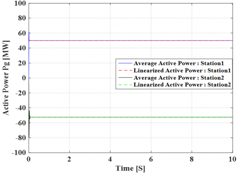
The evolution of the powers transmitted through the two converters of the VSC system is given in Figure 11. In accordance with this figure, the complementarity of the waveforms of powers transmitted through the two stations during time simulation is assured. The DC link was transferring 50 [MW] from Station 2 which controls the power transfer to station 1 which controls the DC bus voltage.
In addition, it is notable that the evolution of the linearized active power in each station is similar to the evolution of the average model. Hence, the linearized active power controller model in VSC-HVDC link is proved.
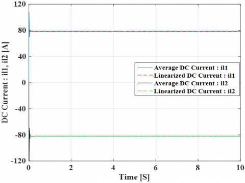
Whenever station 2 changes its power flow, there is an excess of the current il2 into the DC cable from the sending station 2 to the receiving station 1. Thus, the negative sign of the current il2 is clarified. While the current il1 flows in the opposed path.
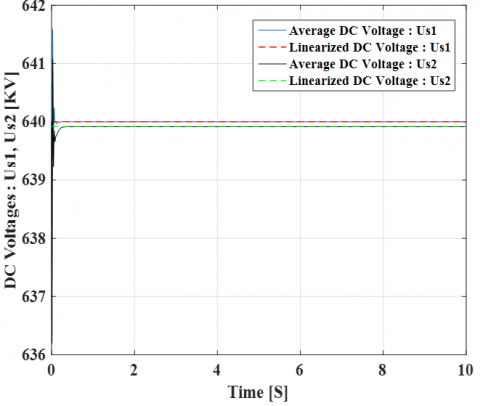
There is no remarkable difference between the waveform of the DC bus voltages Us1 and The DC bus voltages Us2, their curve is constant at 640 [KV] during time simulation as presented in Figure 13. In fact, the balance between the power generated by the station 2 and the power absorbed by the station 1 empowers the DC bus voltage to be adjusted to its reference value. Thus, this pace shows the effectiveness of the control loop used.
In addition, it is notable that the evolution of the linearized DC voltage in each station is similar to the evolution of the average model. Hence, the linearized voltage controller model in VSC-HVDC link is proved.
Figure 11. State space model validation of the active power controller in VSC-HVDC link
Figure 12. DC current
Figure 13. Voltage controller of the VSC-HVDC link state space model validation
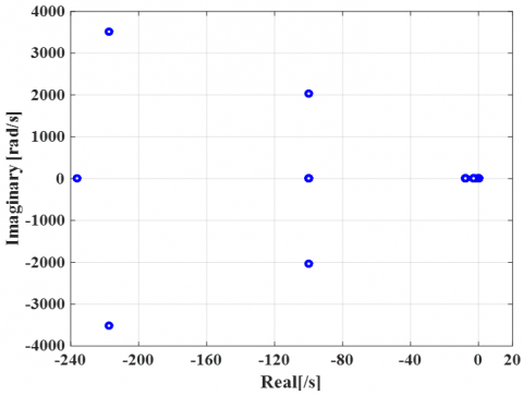
Figure 14. Root locus of the VSC-HVDC link
Table 1. Eigenvalues of the VSC-HVDC system
|
Number |
Eigenvalues |
|
1 |
-1.297 |
|
2 |
-2.838 |
|
3 |
-2.885 |
|
4 |
-2.885 |
|
5 |
-2.885 |
|
6 |
-7.778 |
|
7 |
-7.778 |
|
8 |
-7.778 |
|
9 |
-7.82 |
|
10 |
-100.002 |
|
11 |
-100.002 |
|
12 |
-100.002 |
|
13 |
100.125+2038j |
|
14 |
-100.125+351j |
|
15 |
-217.48+351j |
|
16 |
-217.48-351j |
|
17 |
0 |
|
18 |
0 |
|
19 |
-1.39e-43 |
|
20 |
-3.410e-42 |
|
21 |
-236.17 |
|
22 |
-19997.55 |
|
23 |
-19997.55 |
|
24 |
-9999999.99 |
As conclusion, we approved that the global state space model of the VSC-HVDC is validated. After that, the stability of the VSC-HVDC system will be checked by the eigenvalue-based Stability analysis.
Eigenvalues of the state matrix are resumed in Table 1.
The number of eigenvalues is equal to the number of states variables: 10 for the current controller, 2 for the active power controller, 4 for the reactive power controller, 2 for the voltage power controller, 2 for the smoothing reactor, and 4 for the DC cable.
The plot of Figure 14 illustrates the roots referred to the total VSC-HVDC system, we notice that all the eigenvalues have a negative real part, the root is clearly oscillating but finally converges until reaching the abscissa axis. Which prove that the VSC-HVDC system is asymptotically stable.
Small-signal stability analyses (SSSA) becomes essential in the design of HVDC controllers in order to enhance their flexibility to faults, and to boost their aptitude to contribute to power grid operation.
The stability of two terminal VSC-HVDC system using the small signal stability technique for a linearized state space model is studied in this paper. The state space model of each subsystem was developed then a connection between each block was made to create a global linear state space model. The study of eigenvalues associated to the global linearized state space system is automatically used to improve the stability of the VSC-HVDC link. This work will help us to develop a generic method, with a view of providing flexible models to study the stability of a multi-terminal MTDC grid.
|
VSC |
Voltage Source Converter |
|
HVDC |
High Voltage Direct Current |
|
AC |
Alternating Current |
|
DC |
Direct Current |
|
LCC |
Line-commutated converter |
|
HVAC MPPT |
High Voltage Alternating Current Maximum Power Point Tracking |
|
SSSA PWM PLL |
Small Signl Stability Analysis Pulse-Width Modulation Phase Lock Loop |
|
PI |
Proportional Integral |
|
TF |
Transfer Function |
The control loops characteristics are resumed in this table.
Table 2. VSC control loop characteristics
|
|
Response Time [MS] |
The damping ratio |
|
Current loop |
10 |
0.7 |
|
Power loop |
200 |
- |
|
Voltage loop |
100 |
0.7 |
|
PLL |
1 |
0.7 |
For a DC transmission, two cables buried beneath the ground, are used. One for the positive pole and the other for the negative pole (Table 3).
Table 3. Cable parameters
|
|
Cable 320 kV 2500 mm² |
|
Cable section [mm²] |
2500 |
|
Nominal current [A] |
1800-2700 |
|
Rc1: Core resistance[mΩ/km] |
5.3 |
|
Lc1: Core inductance [mH/km] |
3.6 |
|
Lc2: Screen inductance [mH/km] |
3.5 |
|
Mc12: Core-screen mutual inductance [mH/km] |
3.5 |
|
Rc2: Screen resistance [mΩ/km] |
60.2 |
|
Mc12: Core Screen mutual inductance [mH/Km] |
0.15 |
|
Gc1, Gc2: Core-to-ground conductances [μS/km] |
0.06 |
|
Cc1, Cc2: Core to ground Capacitances [μF/km] |
0.24 |
[1] Singh, S., Singh, M., Kaushik, S.C. (2016). A review on optimization techniques for sizing of solar-wind hybrid energy systems. International Journal of Green Energy, 13(15): 1564-1578. https://doi.org/10.1080/15435075.2016.1207079
[2] Wang, Y.S., Gao, J., Xu, Z.W., Li, L.X. (2020). A short-term output prediction model of wind power based on deep learning of grouped time series European. Journal of Electrical Engineering, 22(1): 29-38. https://doi.org/10.18280/ejee.220104
[3] Hadaeghi, A., Samet, H., Ghanbari, T. (2019). Multi SVR Approach for Fault Location in Multi-terminal HVDC Systems. International Journal of Renewable Energy Research (IJRER), 9(1): 194-206.
[4] Flourentzou, N., Agelidis, V.G., Demetriades, G.D. (2009). VSC-based HVDC power transmission systems: An overview. IEEE Transactions on power electronics, 24(3): 592-602. https://doi.org/10.1109/TPEL.2008.2008441
[5] Vu, T.T.N., Teyssèdre, G., Roy, S.L., Anh, T.T., Trần, T.S., Nguyen, X.T., Nguyễn, Q.V. (2019). The challenges and opportunities for the power transmission grid of Vietnam. European Journal of Electrical Engineering, 21(6): 489-497. https://doi.org/10.18280/ejee.210602
[6] Asplund, G. (2007). Ultra high voltage transmission. ABB Review, (2): 22-27.
[7] Oscullo, J., Gallardo, C. (2019). Tuning and location of PSS in multimachine power system with state feedback control for electromechanical oscillation damping control. European Journal of Electrical Engineering, 21(6): 499-507. https://doi.org/10.18280/ejee.210603
[8] Kundur, P., Paserba, J., Ajjarapu, V., Andersson, G., Bose, A., Canizares, C. (2004). Definition and classification of power system stability IEEE/CIGRE joint task force on stability terms and definitions. IEEE transactions on Power Systems, 19(3): 1387-1401. https://doi.org/10.1109/TPWRS.2004.825981
[9] Kalcon, G.O., Adam, G.P., Anaya-Lara, O., Lo, S., Uhlen, K. (2012). Small-signal stability analysis of multi-terminal VSC-based DC transmission systems. IEEE Transactions on Power Systems, 27(4): 1818-1830. https://doi.org/10.1109/TPWRS.2012.2190531
[10] Mbaabu, L.M., Kaberere, K.K., Hinga, P.K. (2019). Performance analysis of the voltage source converter based high voltage direct current link on small signal stability. International Journal of Scientific & Technology Research, 8(10): 1719-1724.
[11] Song, Y., Breitholtz, C. (2015). Nyquist stability analysis of an AC-grid connected VSC-HVDC system using a distributed parameter DC cable model. IEEE Transactions on Power Delivery, 31(2): 898-907. https://doi.org/10.1109/TPWRD.2015.2501459
[12] Dadjo Tavakoli, S., Prieto-Araujo, E., Sánchez-Sánchez, E., Gomis-Bellmunt, O. (2020). Interaction assessment and stability analysis of the MMC-Based VSC-HVDC link. Energies, 13(8): 2075. https://doi.org/10.3390/en13082075
[13] Patino, M., Hohn, S., Dimitrovski, R., Luther, M. (2019). Methodology for state-space modelling of power electronic elements in modern electrical energy systems. 15th IET International Conference on AC and DC Power Transmission (ACDC 2019). https://doi.org/10.1049/cp.2019.0048
[14] Wu, W., Zhou, L., Chen, Y., Luo, A., Dong, Y., Zhou, X., Guerrero, J.M. (2018). Sequence-impedance-based stability comparison between VSGs and traditional grid-connected inverters. IEEE Transactions on Power Electronics, 34(1): 46-52. https://doi.org/10.1109/TPEL.2018.2841371
[15] Zhu, M., Nian, H., Xu, Y., Chen, L. (2018). Impedance-based stability analysis of MMC-HVDC for offshore DFIG-based wind farms. In 2018 21st International Conference on Electrical Machines and Systems (ICEMS), pp. 1139-1144. https://doi.org/10.23919/ICEMS.2018.8549246
[16] Xu, L., Yao, L. (2011). DC voltage control and power dispatch of a multi-terminal HVDC system for integrating large offshore wind farms. IET Renewable Power Generation, 5(3): 223-233. https://doi.org/10.1049/iet-rpg.2010.0118
[17] Beerten, J., Van Hertem, D., Belmans, R. (2011). VSC MTDC systems with a distributed DC voltage control-A power flow approach. 2011 IEEE Trondheim PowerTech, Trondheim, pp. 1-6. https://doi.org/10.1109/PTC.2011.6019434
[18] Chaudhuri, N.R., Majumder, R., Chaudhuri, B., Pan, J. (2011). Stability analysis of VSC MTDC grids connected to multimachine AC systems. IEEE Transactions on Power Delivery, 26(4): 2774-2784. https://doi.org/10.1109/TPWRD.2011.2165735
[19] Alsseid, A.M., Jovcic, D., Starkey, A. (2011). Small signal modelling and stability analysis of multiterminal VSC-HVDC. In Proceedings of the 2011 14th European Conference on Power Electronics and Applications, pp. 1-10. https://doi.org/10.1149/1.3631510
[20] Pinares, G., Bongiorno, M. (2015). Modeling and analysis of VSC-based HVDC systems for DC network stability studies. IEEE Transactions on Power Delivery, 31(2): 848-856. https://doi.org/10.1109/TPWRD.2015.2455236
[21] Kharade, J.M., Savagave, D.N.G. (2017). A review of HVDC converter topologies. International Journal of Innovative Research in Science, Engineering and Technology, 6(2): 1822-1830. https://doi.org/10.15680/IJIRSET.2017.0602054
[22] Shinoda, K., Benchahib, A. (2014). Modelling of a multiterminal HVDC network for dynamic stability analysis under faults. Ecole Centrale de Lille-L2EP CS 20048, 59651 Villeneuve d'Ascq.
[23] Rault, P., Colas, F., Guillaud, X., Nguefeu, S. (2012). Method for small signal stability analysis of VSC-MTDC grids. 2012 IEEE Power and Energy Society General Meeting, San Diego, CA, pp. 1-7. https://doi.org/10.1109/PESGM.2012.6345318
[24] Rekik, A., Boukettaya, G. (2018). Modelling, Control and simulation of VSC-HVDC systems. In 2018 15th International Multi-Conference on Systems, Signals & Devices (SSD), pp. 721-726. https://doi.org/10.1109/SSD.2018.8570414
[25] Peralta, J., Saad, H., Dennetière, S., Mahseredjian, J. (2012). Dynamic performance of average-value models for multi-terminal VSC-HVDC systems. 2012 IEEE Power and Energy Society General Meeting, San Diego, CA, pp. 1-8. https://doi.org/10.1109/PESGM.2012.6345610
[26] Karawita, C., Annakkage, U.D. (2009). A hybrid network model for small signal stability analysis of power systems. IEEE Transactions on Power Systems, 25(1): 443-451. https://doi.org/10.1109/TPWRS.2009.2036709
[27] Alsseid, A.M., Jovcic, D., Starkey, A. (2011). Small signal modelling and stability analysis of multiterminal VSC-HVDC. In Proceedings of the 2011 14th European Conference on Power Electronics and Applications, pp. 1-10. https://doi.org/10.1149/1.3631510
[28] Heidari, R., Seron, M.M., Braslavsky, J.H. (2015). Eigenstructure assignment for component wise ultimate bound minimization in discrete-time linear systems. IEEE Transactions on Automatic Control, 61(11): 3669-3675. https://doi.org/10.1109/TAC.2015.2513367