Liqing Xiao
OPEN ACCESS
To satisfy the accuracy of image reconstruction, this paper carries out offline optimization of the Hessian matrix in the modified Newton-Raphson algorithm (MNRA) for image reconstruction of electrical resistance tomography (ERT). Firstly, the selection strategy of regularization factor, which directly affects the accuracy of the reconstructed image, was discussed in details. Next, the improved particle swarm optimization (PSO) algorithm was adopted to alleviate the ill-posedness of the Hessian matrix through offline optimization. The variables of offline optimization include the radius ratio between each layer of the finite-element model (FE model) to the sensitive field (SF) during the γ-refinement of the ERT, and the positions of the nodes added through element subdivision. The experimental results show that, under the same conditions, the above optimization measure can improve the solution accuracy of the ERT’s inverse problem by alleviating the ill-posedness of the Hessian matrix, which is used to correct the dielectric resistance distribution (DRD) in the SF, without sacrificing the real-time performance of the MNRA.
hessian matrix, regularization factor, ill-posedness, γ-refinement, element subdivision
Electrical resistance tomography (ERT) [1-10] is a branch of electrical tomography, alongside with electrical capacitance tomography (ECT) [11-16], electrical impedance tomography (EIT) [17-25] and electromagnetic tomography (EMT) [26-29]. Compared with traditional detection methods, this novel real-time detection technique satisfies the high accuracy requirement of modern detection tasks, and enjoys broad application prospects in various fields, namely, two-phase/multi-phase flow, geophysical exploration and biomedicine.
Many algorithms have been developed to reconstruct images accurately, without sacrificing real-time performance. Among them, the modified Newton-Raphson algorithm (MNRA) stands out as a theoretically complete iterative reconstruction algorithm for static images [30]. In the iterative process, the MNRA introduces a Hessian matrix, which contains a regularization factor, to correct the dielectric resistance distribution (DRD) in the sensitive field (SF), and thus effectively overcomes the ill-posedness of sensitivity matrix. The regularization factor directly bears on the quality of the image reconstructed by the MNRA. Currently, the regularization factor is selected in two ways: empirical selection or online real-time calculation. Either approach has certain defects. Lacking theoretical basis, empirical selection cannot guarantee that the image is reconstructed at the accuracy required by the system. Meanwhile, online real-time calculation solves the inverse problem of the ERT, more accurately at the cost of real-time performance, as it increases the computing load of the image reconstruction algorithm. By refining the finite-element model (FE model), Xiao et al. [30] effectively solved the ill-posedness without affecting the real-time performance. However, their approach still faces several defects:
1. The topology of the FE model was not optimized. Under the same conditions, each topology of the FE model corresponds to a specific Hessian matrix with a unique level of ill-posedness, and a distinct solution accuracy of the inverse problem.
2. The positions of the nodes added in the element subdivision process were not optimized.
To overcome the above defects, this paper firstly explores the selection strategy of the regularization factor. On this basis, the ill-posedness of Hessian matrix was alleviated through offline optimization of the FE model topology during the γ-refinement of the ERT's forward problem, and the positions of the nodes added through element subdivision. In this way, the author greatly improved the accuracy of the MNRA in image reconstruction.
The principle of the MNRA is as follows [30]:
Step 1. Initialize the DRD $\rho^{(0)}$ in the SF.
Step 2. Calculate the effective boundary voltage of the SF corresponding to the DRD $\rho^{(k)}$ in the k -th iteration of the MNRA: $\boldsymbol{v}^{(k)}=f\left(\boldsymbol{\rho}^{(k)}\right)$ .
Step 3. Compute the error of the MNRA by:
$e_{r r o r}=\frac{1}{2}\left(\left\|v^{(k)}-v_{0}\right\|_{2}\right)^{2}$ (1)
where, $\boldsymbol{v}_{0}$ is the measured effective boundary voltage of the SF.
Step 4. Judge if the MNRA satisfies the termination condition. If not, go to Step 5.
Step 5. Introduce the Hessian matrix with the regularization factor, correct the DRD $\rho^{(k+1)}$ in the SF, and jump back to Step 2:
$\boldsymbol{\rho}^{(k+1)}=\boldsymbol{\rho}^{(k)}+\Delta \boldsymbol{\rho}^{(k+1)}$ (2)
$\begin{aligned} \Delta \rho^{(k+1)}=&-\left\{\left[f^{\prime}\left(\rho^{(k)}\right)\right]^{T} f^{\prime}\left(\rho^{(k)}\right)+\mu^{(k)} E\right\}^{-1} \\ &\left[f^{\prime}\left(\rho^{(k)}\right)\right]^{T}\left(f\left(\rho^{(k)}\right)-v_{0}\right) \end{aligned}$ (3)
where, $\boldsymbol{E}$ is the unit matrix; $\mu^{(k)}$ is the regularization factor adopted by the MNRA in the $k$ -th iteration; $f^{\prime}\left(\boldsymbol{\rho}^{(k)}\right)$ is the sensitivity matrix when the DRD of the SF is $\boldsymbol{\rho}^{(k)}$ ; $\left[f^{\prime}\left(\boldsymbol{\rho}^{(k)}\right)\right]^{T} f^{\prime}\left(\boldsymbol{\rho}^{(k)}\right)+\mu^{(k)} \boldsymbol{E}$ is the Hessian matrix used to correct the DRD.
The offline optimization of the Hessian matrix used to correct the DRD in the SF is carried out during the iteration of the MNRA, based on the selection strategy of the regularization factor, which directly affects the ERT’s image reconstruction accuracy. In this paper, this Hessian matrix is optimized by improved particle swarm optimization (PSO) algorithm. The variables include the radius ratio between each FE model layer to the SF during the γ-refinement of the ERT's forward problem, and the positions of the nodes added through element subdivision. The specific flow of the offline optimization is as follows:
Step 1. Selection of regularization factor
In the MNRA, it is difficult to reconstruct a high-quality image with a fixed regularization factor. This factor should be adjusted reasonably according to the MNRA error (formula (1)) in the iterative process. In the early phase, the algorithm has a large error, i.e. low accuracy in image reconstruction. In this case, the regularization factor should be large enough to ensure the stability of the MNRA, and the solution accuracy of the inverse problem. In the late phase, the algorithm has a small error, i.e. high accuracy in image reconstruction. In this case, the regularization factor should be small enough, such that the reconstructed image reflects the actual DRD in the SF. Of course, the regularization factor should not be too small. Otherwise, the MNRA will diverge in the iterative process. Hence, the minimum value of the regularization factor should be identified rationally, considering the prior knowledge and the FE model accuracy in solving ERT’s forward problem.
To sum up, during the iteration of the MNRA, the $\left\{\left[f^{\prime}(\boldsymbol{\rho})\right]^{T} f^{\prime}(\boldsymbol{\rho})+\mu^{(k)} \boldsymbol{E}\right\}^{-1} \cdot\left[f^{\prime}(\boldsymbol{\rho})\right]^{T}$ should be calculated offline and saved to facilitate the offline optimization of the Hessian matrix, which is used to correct the DRD in the SF. Meanwhile, the small value interval of the regularization factor should be expanded to narrow its large value interval. In this paper, the maximum and minimum values of the regularization factor are both configured, with the median value satisfying the log-uniform distribution:
$l=p / q^{k}$ (4)
$\mu^{(k)}=\left\{\begin{array}{ll}{a^{-d}} & {l<a^{-d}} \\ {a^{-b}} & {l \geq a^{-b}} \\ {a^{-h_{1}}} & {a^{-h_{1}} \leq l<a^{-h_{2}}}\end{array}\right.$ (5)
where, a, b, d, p and $q$ are positive numbers that satisfy $a>1$ , $d>1, q>1$ and $d>b$ ; $h_{1}$ and $h_{2}$ can be calculated by:
$h_{1}=b+\frac{d-b}{t-1} \cdot(m-1) \quad m=2, \cdots t$ (6)
$h_{2}=b+\frac{d-b}{t-1} \cdot(m-2) \quad m=2, \cdots t$ (7)
where, $t$ is a positive integer greater than 2.
Step 2. Offline optimization of Hessian matrix
The global element subdivision of the FE model [30] was adopted to improve the data transmission efficiency between the FE model adopted for ERT’s forward problem and the FE model adopted to correct the DRD in the SF.
The previous experiments have shown that, under the same conditions, the MNRA can solve the inverse problem more accurately by updating the sensitivity matrix. Hence, the following strategy can be implemented to enhance the quality of reconstructed image without sacrificing the real-time performance of the MNRA: First, different DRDs should be set up in the SF according to rich prior knowledge (especially in biomedicine), and the corresponding regularization factors should be computed by formulas (4)~(7). On this basis, the Hessian matrices should be established corresponding to the DRDs and regularization factors. Once every few iterations, the correlation coefficient should be computed between the optimal reconstructed image of the MNRA and the reconstructed image corresponding to each DRD, and used to judge whether the Hessian matrix needs to be updated. The offline optimization of the Hessian matrix involves the following steps:
Step 1. Set up parameters like a , b , d , p , q , k and t .
Step 2. Take the following two items as the variables: the radius ratio between each FE model layer to the SF during the γ-refinement of the ERT's forward problem, and the positions of the nodes added through element subdivision. Set up the fitness function as:
$F(Y)={}^{1}/{}_{\sum\limits_{i=1}^{w}{{{\eta }_{i}}\cdot cond({{H}_{i}})}}$ (8)
where, $\eta_{i}$ is a nonnegative weight; $\text { cond }$ is the conditional number; $\boldsymbol{H}_{i}$ is the Hessian matrix corresponding to each DRD in the SF and each regularization factor; w is the number of Hessian matrices; $\boldsymbol{Y}$ is a variable representing the radius ratio between each FE model layer to the SF during the γ-refinement of the ERT's forward problem, and the positions of the nodes added through element subdivision.
Moreover, conduct offline optimization of the Hessian matrix through improved PSO algorithm. During the optimization, update the particle velocity and position by:
$\left\{\begin{array}{l}{\boldsymbol{V}_{i}=\omega \times \boldsymbol{V}_{i}+c_{1} \times \text {rand} 1 \times\left(\text {pbest}_{i}-\boldsymbol{X}_{i}\right)} \\ {+c_{2} \times \text {rand} 2 \times\left(\text {gbest}_{g}-\boldsymbol{X}_{i}\right)} \\ {\boldsymbol{X}_{i}=\boldsymbol{X}_{i}+\boldsymbol{V}_{i}}\end{array}\right.$ (9)
where, $\boldsymbol{X}_{i}$ and $V_{i}$ are the position vector and velocity vector of particle i, respectively; pdestiand gbestg are the individual best-known solution and global best-known solution, respectively; w is the inertial weight; $c_{1} \text { and } c_{2}$ are learning factors; rand 1 and rand 2 are random numbers in (0, 1).
Step 3. To improve the real-time performance of the MNRA, carry out offline calculation and storage of the following term based on the optimization results in the previous step: $\left\{\left[f^{\prime}(\rho)\right]^{T} f^{\prime}(\rho)+\mu^{(k)} E\right\}^{-1} \cdot\left[f^{\prime}(\rho)\right]^{T}$ .
In our simulation experiment, some parameters are configured as follows: the maximum number of iterations for the improved PSO algorithm for offline optimization of the Hessian matrix and that for the MNRA were both set to 200; the upper and lower bounds of the inertial weight were set to 0.90 and 0.10, respectively; for the efficiency of offline optimization, the DRDs in the SF were assumed as continuous uniform distributions, and the weight of each Hessian matrix $\eta_{i}$ was set to 1.00; considering accuracy and time consumption, the FE model was designed with 8 layers, and the radius of the SF was normalized; the regularization factors of the MNRA iterations were set to 10-1, 10-2…10-8 according to parameters like p =0.50, q =1.15, a =10, b =1, d =8 and t =8.
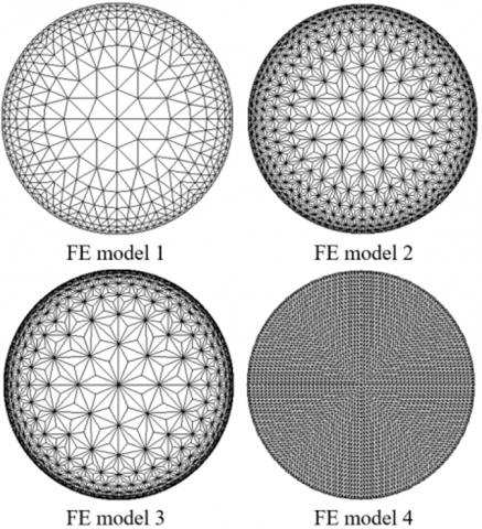
Figure 1. FE models
Under the above settings, the FE model topology corresponding to the optimal result of the offline optimization of Hessian matrix, as well as the positions of the nodes added through element subdivision are recorded as FE model 3 in Figure 1. FE model 1 was proposed by Xiao et al. [31], which can effectively enhance the solution accuracy of the forward problem. FE model 2 was also developed by Xiao et al. [30], which can satisfactorily alleviate the ill-posedness of Hessian matrix. In FE model 2, the nodes added through element subdivision are the centroids of triangular elements. FE model 4 is an FE model that computes the measured effective boundary voltages under different model settings, without committing the inverse crime. To minimize the error between the calculated and theoretical values of the FE model corresponding to each DRD in the SF, FE model 4 performs offline optimization of the radius of the second outmost layer, and assumes that the DRD is uniform in the other layers.
When the regularization factor was set to 10-1, 10-2…10-8, respectively, the mean conditional number of the Hessian matrices corresponding to FE model 1, FE model 2 and FE model 3 was 2.9720×10⁵, 9.9067×10⁴ and 8.2721×10⁴, respectively. In other words, FE model 3, through offline optimization by the improved PSO algorithm, reduced the mean conditional number of Hessian matrices by 72.1666% from that of FE model 1 and 16.4999% from that of FE model 2. This means FE model 3 effectively alleviated the ill-posedness of Hessian matrix and thus enhanced the MNRA’s solution accuracy of the inverse problem.
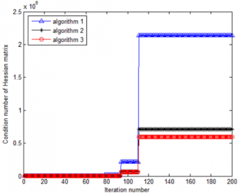
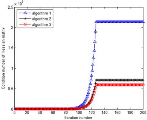
Figure 2 shows how the ill-posedness of Hessian matrix, which is adopted to correct the DRD in the SF, varies through the iterations of the MNRA. Note that Algorithms 1~3 are the Hessian matrices corresponding to the MNRA coupled with FE model 1, FE model 2 and FE model 3, respectively; (a) means the regularization factors are computed by formulas (4)~(7); (b) means the regularization factors are only computed by formula (4).
(a)
(b)
Figure 2. Variation of the ill-posedness in the iterative process
As shown in Figure 2(a), the Hessian matrices optimized by our approach (Algorithm 3) achieved the smallest conditional number at any number of iterations of the MNRA. This means our offline optimization strategy can ensure that the MNRA operates stably and the resolution of reconstructed image can be promoted. It can be seen from Figure 2(b) that our local optimization strategy of Hessian matrix also applies to regularization factors other than 10-1, 10-2…10-8. However, when the regularization factors were only computed by formula (4), the local optimization effect was suppressed. Thus, the offline calculation and storage of $\left\{\left[f^{\prime}(\boldsymbol{\rho})\right]^{T} f^{\prime}(\boldsymbol{\rho})+\mu^{(k)} \boldsymbol{E}\right\}^{-1} \cdot\left[\boldsymbol{f}^{\prime}(\boldsymbol{\rho})\right]^{T}$ only suit systems with low requirements on real-time performance.
In addition, when the sensitivity matrix remained unchanged, the real-time performance of the MNRA is mainly affected by the computing load of correcting the DRD in the SF, under the same experimental conditions. Under our local optimization strategy of Hessian matrix, the $\left.\left[f^{\prime}(\boldsymbol{\rho})\right]^{T} f^{\prime}(\boldsymbol{\rho})+\mu^{(k)} \boldsymbol{E}\right\}^{-1} \cdot\left[f^{\prime}(\boldsymbol{\rho})\right]^{T}$ is computed and saved offline. Under the same experimental conditions (Intel® Core™2 Duo Processor T8100; frequency: 2.10GHz; memory: 3.00GB), our strategy reduced the time consumption in each correction of DRD in the SF from 0.8750-0.8900s to 3.1000×10⁻⁴-4.7000×10⁻⁴s. In this way, the real-time performance of the MNRA is effectively improved, without sacrificing the solution accuracy of the inverse problem.
Next, six different models were constructed (Figure 3a) to verify the effectiveness of our local optimization strategy of Hessian matrix in enhancing the quality of the image reconstructed by the MNRA. The images reconstructed by different MNRAs are compared in Figures 3b~3e and Tables 1~2. Note that Algorithm 4 is the MNRA adopting the Hessian matrices of FE model 3 in Figure 1 and an empirical regularization factor.
Figure 3. Preset models and images reconstructed by different algorithms
The accuracy of image reconstruction was evaluated by two indices: relative error $e$ and correlation coefficient $\rho$ :
$e=\frac{\|g-\hat{g}\|_{2}}{\|g\|_{2}} \times 100 \%$ (10)
$\rho=\frac{\sum_{i=1}^{L}\left(\hat{\boldsymbol{g}}_{i}-\overline{\hat{g}}\right) \cdot\left(\boldsymbol{g}_{i}-\bar{g}\right)}{\sqrt{\sum_{i=1}^{L}\left(\hat{\boldsymbol{g}}_{i}-\overline{\hat{g}}\right)^{2} \sum_{i=1}^{L}\left(\boldsymbol{g}_{i}-\bar{g}\right)^{2}}}$ (11)
where, $\boldsymbol{g}$ is the preset DRD; $\widehat{g}$ is the reconstructed DRD; L is the number of triangular elements in each model; $\bar{g} \text { and } \overline{\hat{g}}$ are the mean values of $g \text { and } \widehat{g}$ , respectively.
Table 1. Comparison of relative errors (%)
|
Preset images |
Algorithm 1 |
Algorithm 2 |
Algorithm 3 |
Algorithm 4 |
|
Image a |
43.8854 |
41.5316 |
31.5779 |
38.3912 |
|
Image b |
26.8399 |
24.6968 |
18.9752 |
22.2840 |
|
Image c |
39.3645 |
31.8230 |
26.8765 |
30.7501 |
|
Image d |
50.2000 |
48.4003 |
41.4398 |
44.0861 |
|
Image e |
52.2830 |
50.2572 |
43.8958 |
46.1671 |
|
Image f |
50.8244 |
47.5660 |
38.9770 |
43.7200 |
|
Mean |
43.8995 |
40.7125 |
33.6237 |
37.5664 |
|
Preset images |
Algorithm 1 |
Algorithm 2 |
Algorithm 3 |
Algorithm 4 |
|
Image a |
0.9286 |
0.9437 |
0.9649 |
0.9337 |
|
Image b |
0.8695 |
0.8871 |
0.9186 |
0.8867 |
|
Image c |
0.8629 |
0.8805 |
0.9335 |
0.9148 |
|
Image d |
0.8236 |
0.8609 |
0.8884 |
0.8660 |
|
Image e |
0.8305 |
0.8454 |
0.8678 |
0.8339 |
|
Image f |
0.7962 |
0.8168 |
0.8385 |
0.8073 |
|
Mean |
0.8519 |
0.8724 |
0.9020 |
0.8737 |
As shown in Tables 1~2, when the regularization factors were all selected by formulas (4)-(7) in the MNRA iteration process, Algorithm 1 failed to reconstruct images desirably, due to the relatively large conditional number of the Hessian matrix used to correct the DRD in the SF: the relative error was high (mean: 43.8995%) and the correlation coefficient was small (mean: 0.8519).
Algorithm 2 alleviated the ill-posedness of Hessian matrix by refining the FE model, thus enhancing the solution accuracy of the inverse problem: the mean relative error was down by 7.2598%, and the mean correlation coefficient was up by 2.4064%, from the levels of Algorithm 1.
Algorithm 3 further reduced the ill-posedness of Hessian matrix through offline optimization of the radius ratio between each FE model layer to the SF during the γ-refinement of the ERT's forward problem, and the positions of the nodes added through element subdivision, and thereby further improved the accuracy of image reconstruction: the mean relative error was reduced by 17.4119%, and the mean correlation coefficient was increased by 3.3929%, from the levels of Algorithm 2.
Algorithm 4 adopts the same FE model topology to solve the ERT’s forward problem and adds nodes at the same positions through element subdivision. However, the regularization factor of this algorithm was empirically selected and fixed through the iterative process. Hence, Algorithm 4 achieved an image reconstruction accuracy better than that of Algorithms 1 and 2, and poorer than that of Algorithm 3: the mean relative error was 10.4953% higher and the mean correlation coefficient was 3.2391% lower than that of Algorithm 3.
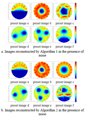
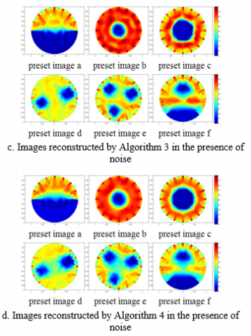
To verify if our offline optimization strategy can enhance the quality of the image reconstructed by the MNRA, the four algorithms were applied to reconstruct the preset models in the presence of noise. The results are compared in Figure 4 and Tables 3-4.
The results in Tables 3 and 4 show that the noise disturbed the solution accuracy of the four different MNRAs in ERT’s inverse problem. Based on offline optimization of Hessian matrix, Algorithm 3 achieved the highest reconstruction accuracy: the mean relative error was 20.5650%, 15.7860% and 8.3251% lower than that of Algorithms 1, 2 and 4, respectively, and the mean correlation coefficient was 7564%, 3.5398% and 3.1914% higher than that of Algorithms 1, 2 and 4, respectively. Hence, Algorithm 3 boasts the best quality of image reconstruction in the presence or absence of noise.
Figure 4. Images reconstructed by different algorithms in the presence of noise
Table 3. Comparison of relative errors in the presence of noise (%)
|
Preset images |
Algorithm 1 |
Algorithm 2 |
Algorithm 3 |
Algorithm 4 |
|
Image a |
48.2505 |
45.4071 |
37.4272 |
41.0747 |
|
Image b |
30.6636 |
29.2343 |
22.0585 |
25.5087 |
|
Image c |
43.0435 |
37.3666 |
31.3782 |
35.0691 |
|
Image d |
52.5580 |
50.5897 |
45.4883 |
47.9869 |
|
Image e |
53.0383 |
52.0269 |
45.0703 |
46.5647 |
|
Image f |
54.0996 |
51.0457 |
42.3092 |
47.8447 |
|
Mean |
46.9423 |
44.2784 |
37.2886 |
40.6748 |
Table 4. Comparison of correlation coefficients in the presence of noise
|
Preset images |
Algorithm 1 |
Algorithm 2 |
Algorithm 3 |
Algorithm 4 |
|
Image a |
0.9162 |
0.9334 |
0.9596 |
0.9282 |
|
Image b |
0.8662 |
0.8745 |
0.9108 |
0.8856 |
|
Image c |
0.8525 |
0.8738 |
0.9161 |
0.8983 |
|
Image d |
0.8093 |
0.8406 |
0.8706 |
0.8390 |
|
Image e |
0.8061 |
0.8301 |
0.8496 |
0.8127 |
|
Image f |
0.7946 |
0.8001 |
0.8284 |
0.8064 |
|
Mean |
0.8408 |
0.8588 |
0.8892 |
0.8617 |
In terms of real-time performance, this paper employs Xiao et al.’s strategy [21] for the iterative process of the MNRA, which ensures the simplicity and efficiency of data transmission between the FE model adopted for ERT’s forward problem and the FE model adopted to correct the DRD in the SF. Therefore, our offline optimization strategy does not affect the real-time performance of the MNRA.
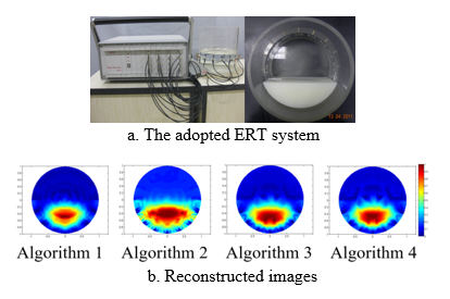
During the experiment, the ERT system designed by Tianjin University was adopted to acquire the effective boundary voltage of the SF (Figure 5a). The images reconstructed by the four algorithms are compared in Figure 5b.
Figure 5. Experimental device and results
For Algorithms 1~4, the relative errors of were 35.9679%, 34.3641%, 30.3435% and 33.5247%, respectively, and the correlation coefficients were 0.6900, 0.7197, 0.7477 and 0.7014, respectively. Compared with Algorithms 1, 2 and 4, Algorithm 3 successfully alleviated the ill-posedness of Hessian matrix and enhanced the quality of reconstructed image, thanks to its dynamic selection of regularization factor and local optimization of Hessian matrix based on two variables (i.e. the radius ratio between each FE model layer to the SF during the γ-refinement of the ERT's forward problem, and the positions of the nodes added through element subdivision).
Among the various ERT techniques, the MNRA is a theoretically complete image reconstruction algorithm, known for its high imaging accuracy. To further enhance the MNRA’s accuracy of image reconstruction, this paper explores the selection strategy of regularization factor in algorithm iteration, and then proposes a local optimization strategy to alleviate the ill-posedness of Hessian matrix with the improved PSO algorithm. The variables of the strategy include the radius ratio between each FE model layer to the SF during the γ-refinement of the ERT's forward problem, and the positions of the nodes added through element subdivision. Experimental results show that our local optimization strategy of Hessian matrix could effectively improve the accuracy of images reconstructed by the MNRA.
This paper is supported by 2018 Annual School-Level Key Scientific Research Project, Huainan Normal University (Grant No.: 2018xj18zd) and 2019 Key Project of Excellent Young Talents Supporting Program of Colleges and Universities, Anhui Province (Grant No.: gxyqZD2019065).
[1] Bobade, V., Evans, G., Eshtiaghi, N. (2019). Bubble rise velocity and bubble size in thickened waste activated sludge: Utilising electrical resistance tomography (ERT). Chemical Engineering Research and Design, 148: 119-128. https://doi.org/10.1016/j.cherd.2019.05.021
[2] Kazemzadeh, A., Ein-Mozaffari, F., Lohi, A. (2019). Mixing of highly concentrated slurries of large particles: Applications of electrical resistance tomography (ERT) and response surface methodology (RSM). Chemical Engineering Research and Design, 143: 226-240. https://doi.org/10.1016/j.cherd.2019.01.018
[3] Vadlakonda, B., Mangadoddy, N. (2018). Hydrodynamic study of three-phase flow in column flotation using electrical resistance tomography coupled with pressure transducers. Separation and Purification Technology, 203: 274-288. https://doi.org/10.1016/j.seppur.2018.04.039
[4] Díaz De Rienzo, M.A., Hou, R., Martin, P.J. (2018). Use of electrical resistance tomography (ERT) for the detection of biofilm disruption mediated by biosurfactants. Food and Bioproducts Processing, 110: 1-5. https://doi.org/10.1016/j.fbp.2018.03.006
[5] Low, S.C., Allitt, D., Eshtiaghi, N., Parthasarathy, R. (2018). Measuring active volume using electrical resistance tomography in a gas-sparged model anaerobic digester. Chemical Engineering Research and Design, 130: 42-51. https://doi.org/10.1016/j.cherd.2017.11.039
[6] Malik, D., Pakzad, L. Experimental investigation on an aerated mixing vessel through electrical resistance tomography (ERT) and response surface methodology (RSM). Chemical Engineering Research and Design, 129: 327-343. https://doi.org/10.1016/j.cherd.2017.11.002
[7] Ren, Z., Kowalski, A., Rodgers, T.L. (2017). Measuring inline velocity profile of shampoo by electrical resistance tomography (ERT). Flow Measurement and Instrumentation, 58: 31-37. https://doi.org/10.1016/j.flowmeasinst.2017.09.013
[8] Singh, B.K., Quiyoom, A., Buwa, V.V. (2017). Dynamics of gas-liquid flow in a cylindrical bubble column: Comparison of electrical resistance tomography and voidage probe measurements. Chemical Engineering Science, 158: 124-139. https://doi.org/10.1016/j.ces.2016.10.006
[9] Vadlakonda, B., Mangadoddy, N. (2017). Hydrodynamic study of two phase flow of column flotation using electrical resistance tomography and pressure probe techniques. Separation and Purification Technology, 184: 168-187. https://doi.org/10.1016/j.seppur.2017.04.029
[10] Son, Y., Kim, G., Lee, S., Kim, H., Min, K., Lee, K.S. (2017). Experimental investigation of liquid distribution in a packed column with structured packing under permanent tilt and roll motions using electrical resistance tomography. Chemical Engineering Science, 166: 168-180. https://doi.org/10.1016/j.ces.2017.03.044
[11] Gupta, S., Loh, K.J. (2018). Monitoring osseointegrated prosthesis loosening and fracture using electrical capacitance tomography. Biomedical engineering letters, 8(3): 291-300. https://doi.org/10.1007/s13534-018-0073-4
[12] Voss, A., Hänninen, N., Pour-Ghaz, M., Vauhkonen, M. (2018). Aku Seppänen. Imaging of two-dimensional unsaturated moisture flows in uncracked and cracked cement-based materials using electrical capacitance tomography. Materials and Structures, 51(3): 1-10. https://doi.org/10.1617/s11527-018-1195-y
[13] Nied, C., Lindner, J.A., Sommer, K. (2017). On the influence of the wall friction coefficient on void fraction gradients in horizontal pneumatic plug conveying measured by electrical capacitance tomography. Powder Technology, 321: 310-317. https://doi.org/10.1016/j.powtec.2017.07.072
[14] Perera, K., Pradeep, C., Mylvaganam, S., Time, R.W. (2017). Imaging of oil-water flow patterns by Electrical Capacitance Tomography. Flow Measurement and Instrumentation, 56: 23-34. https://doi.org/10.1016/j.flowmeasinst.2017.07.002
[15] Kryszyn, J., Wróblewski, P., Stosio, M., Wanta, D., Olszewski, T., Smolik, W.T. (2017). Architecture of EVT4 data acquisition system for electrical capacitance tomography. Measurement, 101: 28-39. https://doi.org/10.1016/j.measurement.2017.01.020
[16] Voss, A., Pour-Ghaz, M., Vauhkonen, M., Seppänen, A. (2016). Electrical capacitance tomography to monitor unsaturated moisture ingress in cement-based materials. Cement and Concrete Research, 89: 158-167. https://doi.org/10.1016/j.cemconres.2016.07.011
[17] Varanasi, S.K., Manchikatla, C., Polisetty, V.G., Jampana, P. (2019). Sparse optimization for image reconstruction in Electrical Impedance Tomography. IFAC PapersOnLine, 52(1):34-39. https://doi.org/10.1016/j.ifacol.2019.06.033
[18] Yoshida, T., Piraino, T., Lima, C.A.S., Kavanagh, B.P., Amato, M.B.P., Brochard, L. (2019). Regional ventilation displayed by electrical impedance tomography as an incentive to decrease positive end-expiratory pressure. American Journal of Respiratory and Critical Care Medicine, 200(7): 933-937. https://doi.org/10.1164/rccm.201904-0797LE
[19] Gregory, H., Tanya, H., Jeffrey, D. (2019). Thoracic electrical impedance tomography to minimize right heart strain following cardiac arrest. Annals of Pediatric Cardiology, 12(3): 315-317. https://doi.org/10.4103/apc.APC_189_18
[20] Simone, S., Giacomo, B., Silvia, V., Ermes, L., Tommaso, M., Giuseppe, F. (2019). A calibration technique for the estimation of lung volumes in nonintubated subjects by electrical impedance tomography. Respiration; International Review of Thoracic Diseases, 98(3): 189-197. https://doi.org/10.1159/000499159
[21] Jiang, Y.D., Soleimani, M. (2019). Capacitively coupled electrical impedance tomography for brain imaging. IEEE transactions on Medical Imaging, 38(9): 2104-2113. https://doi.org/10.1109/TMI.2019.2895035
[22] Miedema, M., Adler A., McCall, Ka.E., Perkins, E.J., van Kaam, A.H., Tingay, D.G. (2019) Electrical impedance tomography identifies a distinct change in regional phase angle delay pattern in ventilation filling immediately prior to a spontaneous pneumothorax. Journal of Applied Physiology, 127(3): 707-712. https://doi.org/10.1152/japplphysiol.00973.2018
[23] Tomicic, V., Cornejo, R. (2019). Lung monitoring with electrical impedance tomography: technical considerations and clinical applications. Journal of Thoracic Disease, 11(7): 3122-3135. https://doi.org/10.21037/jtd.2019.06.27
[24] Murphy, E.K., Skinner, J., Martucci, M., Rutkove, S.B., Halter, R.J. (2019). Toward electrical impedance tomography coupled ultrasound imaging for assessing muscle health. IEEE Transactions on Medical Imaging, 38(6): 1409-1419. https://doi.org/10.1109/TMI.2018.2886152
[25] Marefatallah, M., Breakey, D., Sanders, R.S. (2019). Study of local solid volume fraction fluctuations using high speed electrical impedance tomography: Particles with low Stokes number. Chemical Engineering Science, 203: 439-449. https://doi.org/10.1016/j.ces.2019.03.075
[26] Kaur, C., Singh, P., Sahni, S. (2019). Electroencephalography-based source localization for depression using standardized low resolution brain electromagnetic tomography-variational mode decomposition technique. European neurology, 81: 63-75. https://doi.org/10.1159/000500414
[27] Prinsloo, S., Rosenthal, D.I., Lyle, R., Garcia, S.M., Gabel-Zepeda, S., Cannon, R., Bruera, E., Cohen, L. (2019). Exploratory study of low resolution electromagnetic tomography (LORETA) real-time Z-score feedback in the treatment of pain in patients with head and neck cancer. Brain Topography, 32(2): 283-285. https://doi.org/10.1007/s10548-018-0686-z
[28] Shiina, T., Takashima, R., Pascual-Marqui, R.D., Suzuki, K., Watanabe, Y., Hirata, K. (2018). Evaluation of electroencephalogram using exact low-resolution electromagnetic tomography during photic driving response in patients with migraine. Neuropsychobiology, 77: 1-6. https://doi.org/10.1159/000489715
[29] De Pascalis, V., Scacchia, P. (2017). The behavioural approach system and placebo analgesia during cold stimulation in women: A low-resolution brain electromagnetic tomography (LORETA) analysis of startle ERPs. Personality and Individual Differences, 118: 56-63. https://doi.org/10.1016/j.paid.2017.03.003
[30] Xiao, L.Q., Wang, H.X., Shao, X.G. (2014). Improved Newton-Raphson image reconstruction algorithm based on model refining. Chinese Journal of Scientific Instrument, 35(7): 1546-1554.
[31] Xiao, L.Q., Wang, H.X., Cheng, H.L., Xu, X.J. (2012). Topology optimization of ERT finite element model based on improved GA. Chinese Journal of Scientific Instrument, 33(7): 1490-1496.