Hachelfi Walid* | Rahem Djamel | Meddour Sami | Djouambi Abd Elbaki
OPEN ACCESS
This paper designs a fractional order PID direct torque control strategy for permanent magnet synchronous machine (PSMS) based on on fractional calculus. The fractional order controller to control the speed of the machine was synthesized, referring to Bode’s ideal transfer function. In the controller, the fractional order integrator was approximated by Charef’s method. The fractional PID order control was compared with classical PID control, showing that the former has the better accuracy and robustness. Finally, MATLAB/ SIMULINK simulation proved the advantages of our control strategy under oscillating torque load or magnetic field.
direct torque control (DTC), permanent magnet synchronous machine (PMSM), fractional order PID controller, classical PID controller, Bode’s ideal transfer function, comparison
In recent decades, many scientific applications used fractional calculus and fractional order control for industrial control systems. The research efforts in this domain have increased rapidly due to technological advances and high population density [1-4]. Therefore, many scientific applications such as mechatronics [5], biology [6], photovoltaic [6], automatic voltage regulator [4], robotics and renewable energy systems [7], have been the subject of much research in developed and developing countries. Among these, the fractional electrical machines control [8-10]. The main aim of the control machines and control dynamic process is to enhance the performances and robustness of process control. Therefore, it is necessary to concentrate on the investigation of other control strategies that include fractional calculus and fractional order controllers.
Direct torque control (DTC) is one of the most control strategies, that used in electrical machine drive for different types and investigated in many literatures [11-14]. Unfortunately, this approach has a drawback such as underside torque and speed ripples due to some internal computational defects in control action, this includes switching frequency and voltage vector selection [15-18]. However, Fractional model control has appeared as an attractive and powerful control method in electrical machine drives [8-10]. Due to that, it can be used with several approaches.
Permanent magnets synchronous machine (PMSM) drives play a vitally important role in high performance of the motion control applications [18-21]. The direct torque control or fractional order control is used in the design of PMSM to achieve the best performances [22, 23]. Unluckily, several electromechanical parameters variations are issues in the industrial control machines domain [24-26]. For this problem, several studies are reported [22, 23, 27], to improve the performance and robustness of this type of typical machine drives.
This paper presents a direct torque fractional order control design to PMSM, in this approach, a fractional-order controller PIλDγ [5, 28, 29], is synthesized using Bode’s ideal transfer function as a reference model [30-32]. The proposed technique of the PMSM speed control is compared to the conventional PID controller. Simulation results of the proposed method on a PMSM have been presented to validate the effectiveness of the fractional order direct torque control method.
This paper is organized as follows: Section 2, presents the modelling of the PMSM. Section 3, presents the DTC strategy and the Two-level three-phase voltage source inverter (VSI). Section 4, demonstrate Bode’s ideal transfer function and controller design. In section 5, some application examples of the proposed control strategy are shown. Finally, conclusions remarks are explained in Section 6.
The stator voltage and current equations of the PMSM in the d-q reference is given by [18, 26].
$\left\{\begin{array}{l}{V_{d}=R_{s} i_{d s}+\frac{d \Phi_{d}}{d t}-\Phi_{q} \Omega_{r}} \\ {V_{q}=R_{s} i_{q s}+\frac{d \Phi_{q}}{d t}+\Phi_{d} \Omega_{r}}\end{array}\right.$ (1)
The stator and rotor flux equation can be written in the reference d-q axis as
$\left\{\begin{aligned} \Phi_{d} &=L_{d} i_{d}+\Phi_{m} \\ \Phi_{q} &=L_{q} i_{q} \end{aligned}\right.$ (2)
The electromagnetic torque developed by the PMSM can expressed as
$T_{e}=\frac{3}{2} p\left(\left(\Phi_{d} i_{q s}-\Phi_{q} i_{d s}\right)+\Phi_{m} i_{q s}\right)$ (3)
The electromagnetic torque represented the dynamic behavior of machine can expressed as
$T_{e}=J \frac{d \Omega_{r}}{d t}+f \Omega_{r}+T_{r}$ (4)
In this section a conventional DTC scheme that was applied to PMSM will be discussed. The DTC is based on the theories of field oriented and direct self control. Field oriented control uses space vector theory to optimally control magnetic field orientation and direct self control establishes a unique frequency of inverter operation given a specific dc link voltage and specific stator flux level. The principle of DTC is to stator voltage vectors according to the differences between the reference torque and stator flux linkage and the actual values [22, 23].
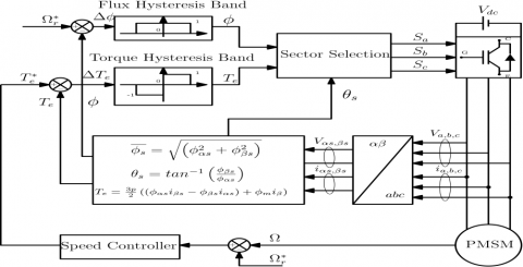
The basic fundamental blocks of the DTC method for PMSM is given in Figure 1. It represents the DTC scheme applied for PMSM. That provides more precise speed control using a PID controller. In other hand, the instantaneous values of stator flux and torque producing are estimated and are controlled by hysteresis controlled directly and independently by properly selecting the inverter switching configuration, hence more responsive and accurate control to your set points [22, 23]. The used of two-level source inverter is based on the switching voltage DTC look-up.
Figure 1. Basic of DTC scheme for PMSM
According to the principle operation of the DTC, there are six non voltage vectors and two zero voltage vectors. The section of six-voltage vectors is made to maintain the torque and stator flux within the limits of two hysteresis bands. The switching selection table for voltage is shown in Table 1 [22, 23].
Table 1. Switching section of the classical DTC
|
|
Section (Si, i=1 to 6) |
||||||
|
Δφ |
ΔTe |
S1 |
S2 |
S3 |
S4 |
S5 |
S6 |
|
1 |
1 |
V2 |
V3 |
V4 |
V5 |
V6 |
V1 |
|
0 |
V7 |
V0 |
V7 |
V0 |
V1 |
V2 |
|
|
-1 |
V6 |
V1 |
V2 |
V3 |
V2 |
V3 |
|
|
0 |
1 |
V5 |
V4 |
V5 |
V6 |
V1 |
V2 |
|
0 |
V0 |
V7 |
V0 |
V7 |
V0 |
V7 |
|
|
-1 |
V5 |
V6 |
V1 |
V2 |
V3 |
V4 |
|
The direct stator flux Фs is derived from Eq. (1). That can be expressed as
$\overrightarrow{\Phi_{s}}=\int \overrightarrow{v_{s}}-R_{s} \overrightarrow{i_{s}}$ (5)
The voltage drop term Rs can be neglected at average and high speed, stator flux variation can be written as
$\frac{\overrightarrow{\Phi_{S}}}{d t}=\int \overrightarrow{V_{S}} \quad \rightarrow$ (6)
Fixing the voltage vector $\vec{V}_{s}=\overrightarrow{0}$ of the Eq. (6), we obtain
$\frac{\overrightarrow{\Phi_{d}}}{d t}=\overrightarrow{0}$ (7)
The approximation magnitude of stator flux as
$\left\{\begin{array}{l}{\Phi_{\alpha s}=\int_{0}^{t}\left(V_{\alpha s}-R_{s} i_{\alpha s}\right) d t} \\ {\Phi_{\beta s}=\int_{0}^{t}\left(V_{\beta s}-R_{s} i_{\beta s}\right) d t}\end{array}\right.$ (8)
The stator flux linkage can be expressed as
$\Phi_{s}=\sqrt{\Phi_{a s}^{2}+\Phi_{\beta s}^{2}}$ (9)
The angular position of the stator flux vector can choose between appropriate vectors set that are depending on the flux position as
$\theta_{S}=\tan ^{-1}\left(\frac{\Phi_{\beta s}}{\Phi_{a s}}\right)$ (10)
The electromagnetic torque calculated by the stator currents and flux measurement as
$T_{e}=\frac{3}{2} p\left(\left(\Phi_{\alpha} i_{\beta s}-\Phi_{\beta} i_{\alpha s}\right)+\Phi_{m} i_{\beta s}\right)$ (11)
The simplified electromagnetic torque equation for an isotropic PMSM (equal direct and quadratic inductance (Ld=Lq) is, namely, can be expressed as
$T_{e}=\frac{3}{2} p \Phi_{m} i_{\beta s}$ (12)
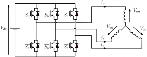
3.1 Voltage source inverter
The three- phases voltage vector Van, Vbn, Vcn of machine are independent, that will be eights different states, so the vector transformation described as [23, 27].
$V_{s}=\sqrt{\frac{2}{3}} U_{c}+\left(S_{a}+S_{b}^{\frac{2 i \pi}{3}}+S_{c}^{\frac{4 i \pi}{3}}\right)$ (13)
The three-phase voltage source inverter VSI are Va, Vband Vdc that alimented the PMSM. The combinations of the each inverter leg are commonly, for this, a logic state Si (i=a,b,c) represents each leg in order to choose an appropriate voltage vector. The simplified representation of inverter with PMSM as shown by Figure 2.
Figure 2. Simplified representation of three-phase voltage inverter
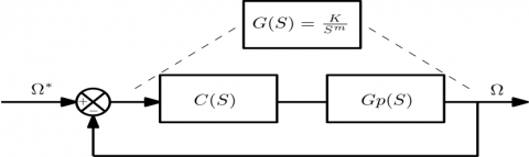
The reference model is based on ideal open loop transfer function used in feedback amplifier that gives the best performance on terms of robustness to the gain variation, the ideal transfer function of Bode is [30-32].
$G(S)=\frac{K}{S^{m}} \cdots 1<m<2 \in R$ 1˂m˂2∊R (14)
where, m is the fractional order integrator.
The Bode’s ideal transfer function (14) exhibits the important properties such as Gain margin -20.m(dB/dec), and a constant phase margin –mπ/2(rad). Besides that, its leading to the iso-damping property. The feedback control system has an important robustness feature even so the variation of the gain K.
Which is an important robustness feature of the feedback control system though the independent of the gain K. By consequence this robustness has motivated some research to consider the unity feedback control system whose forward path transfer function is the Bode’s ideal transfer function, that as shown in Figure 3.
Figure 3. Bode’s ideal transfer function loop
The fractional system exhibits in (14) is the closed-loop transfer function of the control system Eq. (15). Presented in Figure 3 is given by:
$H(S)=\frac{Y(s)}{E(s)}=\frac{G(s)}{1+G(s)}=\frac{1}{1+\left(\frac{s}{w_{14}}\right)^{m}}$ 1˂m˂2∊R (15)
where, the gain crossover frequency $w_{u}=K^{1 / m}$ and the fractional number 1˂m˂2 are fixed according to the desired closed loop performances. the asymptotic approximation of the equation (15), indicates that the magnitude and the phase asymptotically approach a horizontal straight line as (-m20(dB/dec)) and (-mπ/2(rad)), respectively.
Therefore, the constant phase margin $\theta_{m}$ is depending of the fraction value m.
$\theta_{m}=\left(1-\frac{m}{2}\right) \pi,(r a d)$ (16)
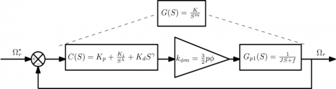
In this paper, the model control scheme is considered as the Bode’s ideal control loop. This is chosen in Figure 4:
Figure 4. Feedback control system
The transfer function control system in open loop is given as
$G(s)=C(s) . G_{p}(s)$ (17)
where, C(S) and Gp(S) are the controller’s and process’s transfer function respectively.
The used fractional order controller has a similar structure with the classical PID controller that is proposed in [2, 24] given as
$C(s)=K_{p}+\frac{K_{i}}{s^{\lambda}}+K_{\dot{d}} S^{\gamma}$ (λ and γ)∊R (18)
The synthesized fractional order controller method is based on the interpretation of the open-loop transfer function C(S) [33], which ensures that the open loop control system Gp(S) behaves like the Bode’s ideal loop as illustrated in Figure 5, thus, we can write [10, 28].
$G(s)=C(s) . G_{p}(s)=\left(K_{p}+\frac{K_{i}}{s^{\lambda}}+K_{d} S^{\gamma}\right) G_{p}(s)=\frac{K}{s^{m}}$ (19)
where, C(s) represent the controller transfer function and Gp(s) represent the plant.
4.1 Fractional order λ, γ
The asymptotic order of the plant Gp(S) at low and high frequency are nb and nh respectively, and the fractional orders λ and γ of the fractional order controller PIλDγcan be given by [33]:
$\left\{\begin{array}{l}{\lambda=m-n_{b}} \\ {\gamma=n_{b}-m}\end{array}\right.$ (20)
4.2 Design of the Parameters Kp, Ki,Kd
The fractional-order Kp, Ki, Kd are calculated by using the tuning method [33]:
$K_{p}=\frac{\left|G_{p}\left(j w_{\max }\right)\right|^{-1}}{\left|1+T_{i}^{\prime}\left(j w_{u}\right)^{-\lambda}+T_{d}^{\prime}\left(j w_{u}\right)^{-\gamma}\right|}$ (21)
$K_{i}=\frac{K_{u}}{\left|\sigma_{p}\left(j w_{m i n}\right)\right| w_{m i n}^{n}}$ (22)
$K_{d}=\frac{K_{u}}{\left|\sigma_{p}\left(j w_{\max }\right)\right| w_{\max }^{\pi}}$ (23)
4.3 Fractional order integrator approximation
The irrational transfer function of the fractional order integrator (14) can be approximated in the frequency band [ωmin, ωmax] by the following rational function [29, 33].
$C(s)=\frac{1}{s^{a}}=\frac{K I}{\left(1+\frac{s}{w_{w}}\right)^{\lambda}}=K I \frac{\Pi_{[-N}^{N-1}\left(1+\frac{s}{z_{l}}\right)}{\prod_{i=0}^{N}\left(1+\frac{s}{p_{s}}\right)}$ (24)
where, piand zi are the poles and zeros of the approximation, 0˂λ˂1 is a positive number.
$\begin{array}{l}{N=\text {Integer }\left[\frac{\log w_{\max }}{p_{0}}+1\right]+1 N=\operatorname{Integer}\left[\frac{\log w_{\max }}{p_{0}}+1\right]} \\ {w_{u}=\sqrt{10^{\left(\frac{\xi}{10} m\right)}-1}} \\ {\qquad K I=\frac{1}{w_{u}^{\lambda}}}\end{array}$
ξ (dB) is the tolerated error between the integration and his approximation.
The singularities of poles pi and zeros zi are given by the flowing formula as
$p_{i}=a b^{i} a p_{0}$ , (i=-1, 0, 1,…, N),
$z_{i}=a b^{i} a p_{0}$ , (i=0, 1,…, N-1).
The parameters a, b, p0 and z0 are:
$\begin{aligned} a=10\left(\frac{y}{10(1-m)}\right), & b=10 \cdot a=10^{\left(\frac{y}{10 m}\right)} \\ p_{0}=w_{u} \sqrt{b}, z_{0}-a p_{0} \end{aligned}$
The irrational transfer fractional function of integrator (14) can be approximated as flowing rational transfer function as
$C(s)=\frac{1}{s^{\lambda}}=\frac{K I}{\left(1+\frac{s}{w_{u}}\right)^{\lambda}}=K I \frac{\prod_{i=N}^{N-1}\left(1+\frac{s}{\left(a b^{i} a p_{0}\right)}\right)}{\prod_{i=0}^{N}\left(1+\frac{s}{\left(a b^{i} p_{0}\right)}\right.}$ (25)
In this section, the parameters values of the PMSM are shown in Table 2, a functional scheme of fractional order control speed is presented, the optimal values of proportional, integral, and derivative gains of classical PID controller and fractional order PID controller are calculus to achieve desired performance ( $\theta_{m}$ , ωu) and meet design requirements.
The proposed fractional order PID controller was compared against a PI controller with same improve performances. Thus, a fair comparison was established between the proposed PID controller to a classical PID controller.
Table 2. Sizes for (PMSM)
|
Motor Parameter |
Symbol |
Value |
|
Nominal power |
Pu |
1,1 (kw) |
|
Pole pairs |
p |
3 |
|
Stator resistance |
Rs |
1.4 (Ω) |
|
Longitudinal inductance |
Ld |
0.0066 (H) |
|
Moment of rotor inertia |
J |
0.00176(Kg.m2) |
|
Quadratic inductance Friction Coefficient |
Lq f |
0.0066 (H) 0.1 |
|
Flux linkage of rotor permanent-magnet |
Фm |
0.1546 (Wb) |
The interested model consists on the closed loop control of speed rotation to follow the Bode’s ideal loop. Thus, the representation of scheme with nominal parameters that are listed in Table 2 is given in Figure 5.
Figure 5. Functional scheme of fractional order control speed
The process Gp(s) of control system is given as:
$\begin{aligned} G_{p}(s) &=K_{\Phi m} \cdot G_{p 1}(s) \\ G_{m}(s) &=\frac{w_{l}^{1.5}}{s^{1.5}}=\frac{70^{1.5}}{s^{1.5}}, S=j w \end{aligned}$ (26)
kФm Design the mechanical torque generated by Electromagnetic torque of (PMSM) given in (3).
$K_{\Phi m}=\frac{3}{2} p \Phi_{m}$ (27)
The transfer function represented the dynamic system that given as
$G_{p}(s)=\frac{K_{\$} m}{0.00176 . S+0.1}$ (28)
So, the process Gp(s) can written as
$G_{p}(s)=\frac{K_{\phi} m}{0.00176 . S+0.1}$ (29)
In a given frequency band [10-4 104], the dynamic performance requirement of our system, can be satisfied for a phase margin θm=45° and a chosen gain crossover frequency $w_{u}=10(r a d / s)$ .
As a result, the Bode’s ideal transfer function can be given as
$G m(s)=\frac{w_{u}^{1.5}}{s^{1.5}}=\frac{70^{1.5}}{s^{1.5}}, S=j w$ (30)
Using (20), we can get
$\left\{\begin{array}{c}{\lambda=1.5} \\ {\gamma=-0.5}\end{array}\right.$ (31)
The values Kp, Ki, Kd of the parameters according to (21, 22 and 23) can be fixed by:
Kp =0.0024; Ki=841.831; Kd=1.4816
Thus, the fractional order controller transfer function as
$G_{F P I I}(s)=0.0024+\frac{84.1831}{s^{1.5}}+1.4816 S^{-0.5}$ (32)
So, the obtained fractional order controller is a proportional parameter Kp, fractional order integrator (I1.5) and second fractional order integrator (I0.5).
Hence from (29 and 32), the open loop transfer function GFPII(s) is given as
$\begin{array}{c}{G_{F P I I}(s)=C_{F P I I} \cdot G(s)} \\ {G_{F P I I}(s)=\frac{0.0017 s^{1.5}+1.0307 S+58,668}{0.00176 S^{2.5}+0.15^{1.5}}}\end{array}$ (33)
And the closed loop transfer function H(s)FPII of (33) is given as
$\begin{array}{c}{H(s)=\frac{G_{F P I I}}{1+G P I(s)}} \\ {H_{F P I I}(s)=\frac{0.017 s^{15}+1.0307 s+58.668}{0.00176 s^{25}+0.1017 s^{5}+0.8745+50.9897}}\end{array}$ (34)
5.1 Performance of fractional PIλDγ controller VS the conventional
The performances of the proposed controller are compared to a classical PI controller, which are designed for the same desired performance, $\theta_{m}=45^{\circ}$ and ωu=70 rad/s.
Using the method of tuning of PID controller to instantly see the optimal parameters of the classical PI, that is a proprietary PID tuning algorithm developed by MATH- WORKS to meet the design objectives such as stability, performance, and robustness’. The obtained optimal PID parameters are given as Kp =0.02358; Ki=15.8802
And the mathematical equation of classical PI controller is given as
$G_{F P I I}(s)=0.02358+\frac{15.8802}{s}$ (35)
Consequently, the open loop transfer function GPI(S) is given as
$\begin{array}{c}{G_{P I}(s)=C_{P I} \cdot G(s)} \\ {G_{P I}(s)=\frac{0.0164 S+11.0479}{0.00176 S^{2}+0.1 S}}\end{array}$ (36)
And the closed loop transfer function H(s)PI of (36) is given as
$\begin{aligned} H(s) &=\frac{G_{P I}}{1+G_{P I}(s)} \\ H_{P I}(s)=& \frac{0.0164 S+11.0479}{0.00176 S^{2}+0.2640 S+11.0479} \end{aligned}$ (37)
5.2 Simulation results
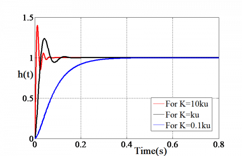
Two simulations examples are presented, in the first test, comparing the fractional order controller, conventional controller and the Bode’s ideal transfer function for various value of K, (K=1;5;10). In the second test, a numerical simulation example is presented by applying the direct torque fractional order control. The obtained results are compared to the conventional method under the variation of the rotor magnets field and the load torque. The reference speed of the machine is fixed at 100rad/s.
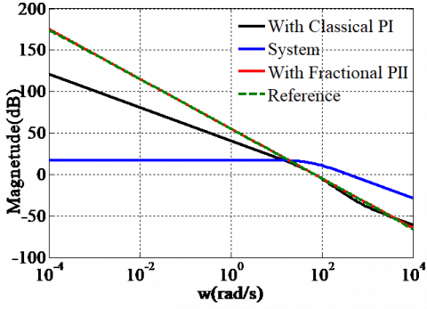
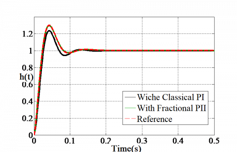
The magnitude plots of reference model, plant transfer function, open loop transfer functions GFPII(s) and open loop transfer functions GPI(s) are shown in Figure 6. We observe that the fractional order control system is overlapped with reference model. Where is not the case with the classical PI. The Figure 7 Shows the step responses of Bode’s ideal loop, closed loop control systems H(s)FPII and H(s)FPI, that is shown a similarity of step responses between the Bode’s ideal loop and fractional order control system.
Figure 6. Magnitude plot of the reference model Gm(s), open loop transfer functions GFPII(s) and open loop transfer functions GPI(s), for m=1.5
Figure 7. Step responses of the reference model Gm(s), open loop transfer functions GFPII(s) and open loop transfer functions GPI(s), for m=1.5
The step responses of the closed loop control systems H(s)FPII and H(s)FPI for various values of static gain K are shown in Figure 8 and Figure 9. It is clear that the first overshoot of the fractional order control system remains constant and realizes fast rise time with good robustness, that characterizes the considered fractional system. Where it is not the case of classical control system.
Figure 8. Step responses of the fractional control system for various values of k
Figure 9. Step responses of the classical control system for various values of k
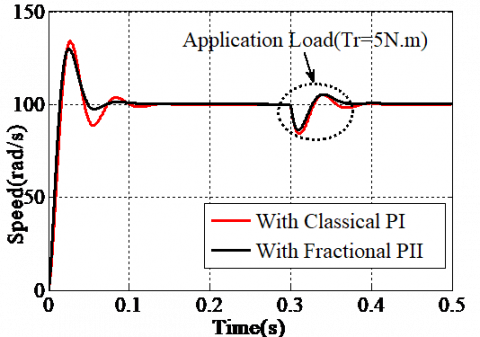
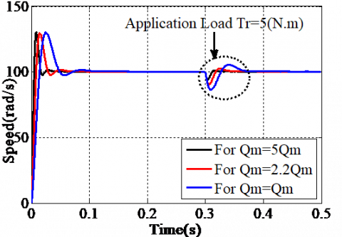
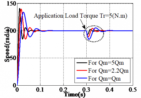
Figure 10. Speed response
The reference of rotor speed of the machine is set to 100rad/s and a load torque is applied to 5N.m at t=0.3s, as shown in Figure 10 and Figure 11. It can observe that the performance indexes such as rise time, maximum overshoot, and steady state error are good level, with a certain improvement in the fractional order control response regarding the overshoot (almost null) and the control signal shape (less oscillations). After applying a load torque Tr=5(N.m) at t=0.3(s) the system response is maintained in a similar manner. The proposed fractional control strategy gives the less oscillatory system for flux magnet variation and application load.
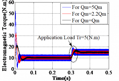
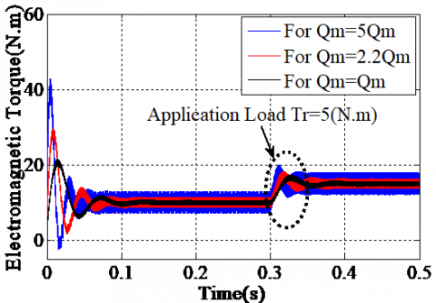
Figure 11. Evolution of electromagnetic torque
The effect of changes in the rotor magnet flux Фm=Qm, (Qm =K. Qm) and application torque load at t=0.3s are shown in Figures. (10-13). It can be seen that the evolution of rotor speed and electromechanical torque for the both control methods.
From Figure 12, the overshoot does not change, the response time has been much faster with the increasing flux magnet respectively. As the load torque applied at t=0.3s, the speed of response is improved.
From Figure 13, the overshoot is variable with a long response time than in Figure 12. Also, it is shown that for load torque at t=0.3s, the speed response obtained is faster with a low overshoot.
Figure 12. Speed responses for different values of Qm of the fractional order DTC
Figure 13. Speed responses for different values of Qm of the classical DTC
The Electromagnetic torque responses of fractional order DTC and classical DTC are shown in Figures (14 and 15) respectively. It can be seen that fractional order DTC offers fast transient responses, good oscillation and very good dynamic responses. But the classical DTC presented the ripple in torque and the torque oscillation is bigger. The oscillation of torque in fractional order DTC is reduced remarkably compared with to classical DTC.
It concluded from this study that fractional order controller can be used to enhance the DTC to maintain the speed overshoot and to reduce the oscillation of the electromagnetic torque with a small ripple.
Figure 14. Evolution of machine electromagnetic torque of the fractional order DTC
Figure 15. Evolution of machine electromagnetic torque for different values Qm of the classical DTC
This paper presents the design of the direct torque fractional order control to PMSM which includes the use of fractional order controller and the robust Bode’s ideal transfer function. The design was simulated using software MATLAB/SIMULINK. Compared to the conventional DTC method, proposed strategy shows good performance and robustness. The speed overshoot is maintained at fixed value and torque ripple is decreased.
|
a, b, p0, z0, y, N |
Approximation parameters |
|
ξ |
Approximation error |
|
is(d,q) |
Stator current in d and q axis |
|
is(α/β) |
Stator current in α and β axis |
|
|
Inductances in d and q axis |
|
m |
Fractional order |
|
nh, nb |
Asymptotic orders |
|
N |
Zero and Pole number |
|
Ni |
Set of point |
|
K |
Gain |
|
Pi, Zi |
Pole and Zero of the approximation |
|
Rs |
Stator resistance |
|
S |
Laplace |
|
S(a,b,c) |
Three switches of too level converter |
|
Te |
Electromagnetic torque |
|
Tr |
Load torque |
|
Uan, Ubn, Ucn |
Tree phase voltage inverter |
|
Vdc |
DC-link voltage |
|
V(d/q) |
Voltage in d and q axis |
|
Vs |
Stator voltage |
|
Vs(α/β) |
Stator voltage in α and β axis |
|
nb and nh |
low and high frequency |
|
|
|
|
Greek symbols
|
|
|
λ, γ |
Non-integer orders |
|
θm |
Phase margin |
|
ωu |
Gain crossover frequency |
|
Ф (d/q) |
Flux linkage in d and q axis |
|
Фm |
Permanent Magnitude flux |
|
Фs |
Stator flux |
|
Фs(α/β) |
Flux linkage in α and β axis |
|
$\Omega_{\mathrm{r}}$ |
Rotor speed |
|
Abbreviations
|
|
|
FOC |
Fractional order Control |
|
PMSM |
Permanent Magnet Synchronous Machine |
|
PID |
Proportional Integral Derivative Controller |
|
PIλDγ |
Fractional Proportional Integral Derivative |
|
DTC |
Direct Torque Control |
|
VSI |
Three-phase Voltage Source Inverter |
[1] Ladaci, S., Bensafia, Y. (2016). Indirect fractional order pole assignment based adaptive control. Engineering Science and Technology, an International Journal, 19(1): 518-530. https://doi.org/10.1016/j.jestch.2015.09.004
[2] Mani., P., Rajan., R., Shanmugam, L., Joo, Y.H. (2018). Adaptive fractional fuzzy integral sliding mode control for PMSM model. IEEE Transactions on Fuzzy Systems, 27(8): 1674-1686. https://doi.org/10.1109/TFUZZ.2018.2886169
[3] Rayalla, R., Ambati, R.S., Gara, B.U.B. (2019). An improved fractional filter fractional IMC-PID controller design and analysis for enhanced performance of non-integer order plus time delay processes. European Journal of Electrical Engineering, 21(2): 139-147. http://doi.org/10.18280/ejee.210203
[4] Aguila-Camacho, N., Duarte-Mermoud, M.A. (2013). Fractional adaptive control for an automatic voltage regulator. ISA Transactions, 52(6): 807-815. https://doi.org/10.1016/j.isatra.2013.06.005
[5] Lamba, R., Singla, S.K., Sondhi, S. (2017). Fractional order PID controller for power control in perturbed pressurized heavy water reactor. Nuclear Engineering and Design, 323: 84-94. https://doi.org/10.1016/j.nucengdes.2017.08.013
[6] Asjad, M.I. (2019). Fractional mechanism with power law (singular) and exponential (non-singular) kernels and its applications in bio heat transfer model. International Journal of Heat and Technology, 37(3): 846-852. http://doi.org/10.18280/ijht.370322
[7] Neçaibia, A., Ladaci, S., Charef, A., Loiseau, J.J. (2015). Fractional order extremum seeking approach for maximum power point tracking of photovoltaic panels. Frontiers Energy, 9(1): 43-53. http://doi.org/10.1007/s11708-014-0343-5
[8] Zouggar, E.O., Chaouch, S., Abdeslam, D., Abdelhamid, A. (2019). Sliding control with fuzzy Type-2 controller of wind energy system based on doubly fed induction generator. Instrumentation Mesure Métrologie, 18(2): 137-146. http://doi.org/10.18280/i2m.180207
[9] Liu, H., Pan, Y., Li, S., Chen, Y. (2017). Adaptive fuzzy backstepping control of fractional-order nonlinear systems. IEEE Transactions on Systems, Man, and Cybernetics: Systems, 47(8): 2209-2217. https://doi.org/10.1109/TSMC.2016.2640950
[10] Singhal, R., Padhee, S., Kaur, G. (2012). Design of fractional order PID controller for speed control of DC motor. International Journal of Scientific and Research Publication, 2(6): 2250-3153.
[11] Ameur, A., Mokhtari, B., Essounbouli, N., Mokrani, L. (2012). Speed sensorless direct torque control of a pmsm drive using space vector modulation based mras and stator resistance estimator. Var. Stator Resist, 1(5). https://doi.org/10.5281/zenodo.1075142
[12] Ammar, A. (2019). Performance improvement of direct torque control for induction motor drive via fuzzy logic-feedback linearization: Simulation and experimental assessment. COMPEL- Int. J. Comput. Math. Electr. Electron. Eng., 38(2): 672-692. https://doi.org/10.1108/COMPEL-04-2018-018
[13] Holakooie, M.H., Ojaghi, M., Taheri, A. (2018). Direct torque control of six-phase induction motor with a novel MRAS-based stator resistance estimator. IEEE Trans. Ind. Electron, 65(10): 7685-7696. https://doi.org/10.1109/TIE.2018.2807410
[14] Kim, J.H., Kim, R.Y. (2018). Sensorless direct torque control using the inductance inflection point for a switched reluctance motor. IEEE Trans. Ind. Electron, 65(12): 9336-9345. https://doi.org/10.1109/TIE.2018.2821632
[15] Araria, R., Negadi, K., Marignetti, F. (2019). Design and analysis of the speed and torque control of IM with DTC based ANN strategy for electric vehicle application. Tec. Ital.-Ital. J. Eng. Sci, 63(2-4): 181-188. http://doi.org/10.18280/ti-ijes.632-410
[16] Liu, Y. (2011). Space vector modulated direct torque control for PMSM. Advances in Computer Science. Intelligent System and Environment, Springer, pp. 225-230. http://doi.org/10.1007/978-3-642-23756-0_37
[17] Mesloub, H., Benchouia, M.T., Goléa, A., Goléa, N., Benbouzid, M.E.H. (2017). A comparative experimental study of direct torque control based on adaptive fuzzy logic controller and particle swarm optimization algorithms of a permanent magnet synchronous motor. Int. J. Adv. Manuf. Technol, 90(1-4): 59-72. http://doi.org/10.1007/s00170-016-9092-4
[18] Jin, S., Jin, W.H., Zhang, F.G., Jing, X.D., Xiong, D.M. (2018). Comparative of direct torque control strategies for permanent magnet synchronous motor. 1st International Conference on Electrical Machines and Systems (ICEMS). http://doi.org/10.23919/ICEMS.2018.8549341
[19] Medjmadj, S. (2019). Fault tolerant control of PMSM drive using Luenberger and adaptive back-EMF observers. European Journal of Electrical Engineering, 21(3): 333-339. http://doi.org/10.18280/ejee.210311
[20] Diao, S., Diallo, D., Makni, Z., Marchand, C., Bisson, J.F. (2015). A differential algebraic estimator for sensorless permanent-magnet synchronous machine drive. IEEE Trans. Energy Convers, 30(1): 82-89. https://doi.org/10.1109/TEC.2014.2331080
[21] Izadfar, H.R., Shokri, S., Ardebili, M. (2007). C. International Conference on Electrical Machines and Systems (ICEMS), pp. 670-674.
[22] C, Xia., S, Wang., X, Gu., Y, Yan., T, Shi. (2016). Direct torque control for VSI-PMSM using vector evaluation factor table. IEEE Trans. Ind. Electron, 63(7): 4571-4583.
[23] Niu, F., Wang, B., Babel, A.S., Li, K., Strangas, E.G. (2016). Comparative evaluation of direct torque control strategies for permanent magnet synchronous machines. IEEE Trans. Power Electron, 31(2): 1408-1424. https://doi.org/10.1109/TPEL.2015.2421321
[24] Ibtissam, B., Mourad, M., Ammar, M., Fouzi, G. (2014). Magnetic field analysis of Halbach permanent magnetic synchronous machine. In the Proceedings of the International Conference on Control, Engineering & Information Technology (CEIT’14), pp. 12-16.
[25] El-Sousy, F.F.M. (2010). Hybrid ∞-neural-network tracking control for permanent-magnet synchronous motor servo drives. IEEE Transactions on Industrial Electronics, 57(9): 3157-3166. https://doi.org/10.1109/TIE.2009.2038331
[26] Harahap, C.R., Saito, R., Yamada, H., Hanamoto, T. (2014). Speed control of permanent magnet synchronous motor using FPGA for high frequency SiC MOSFET inverter. Journal of Engineering Science and Technology, 11-20.
[27] Buja, G.S., Kazmierkowski, M.P., (2004). Direct torque control of PWM inverter-fed AC motors-a survey. IEEE Transactions on Industrial Electronics, 51(4): 744-757. https://doi.org/10.1109/TIE.2004.831717
[28] Charef, A., Assabaa, M., Ladaci, S., Loiseau, J.J. (2013). Fractional order adaptive controller for stabilised systems via high-gain feedback. IET Control Theory Appl, 7(6): 822-828. https://doi.org/10.1049/iet-cta.2012.0309
[29] Charef, A. (2006). Analogue realisation of fractional-order integrator, differentiator and fractional PIλDμ controller. IEE Proc.-Control Theory Appl, 153(6): 714-720. https://doi.org/10.1049/ip-cta:20050019
[30] Bode, H.W. (1945). Network Analysis and Feedback Amplifier Design. R. E. Krieger Pub. Co.
[31] Dogruer, T., Tan, N. (2018). PI-PD controllers design using Bode’s ideal transfer function. Proceedings of International Conference on Fractional Differentiation and its Applications (ICFDA) 2018. http://doi.org/10.2139/ssrn.3271384
[32] Al-Saggaf, U.M., Mehedi, I.M., Mansouri, R., Bettayeb, M. (2016). State feedback with fractional integral control design based on the Bode’s ideal transfer function. International Journal of Systems Science, 47(1): 149-161. https://doi.org/10.1080/00207721.2015.1034299
[33] Djouambi, A., Charef, A., Bouktir, T. (2005). Fractional order robust control and PIα Dβ controllers. WSEAS Transactions on Circuits Systems, 4(8): 850-857.