Slimane Medjmadj
OPEN ACCESS
In this paper, we propose to design a sensorless controller that can cope both with performance and robustness by the hybridization of two controllers. The strategy introduced in this paper includes the sensorless active fault tolerant controller of the PMSM drive at high speed. It is built with the combination of a vector controller, two virtual sensors: Luenberger and adaptive back-EMF observers, and a voting algorithm using Newton-Raphson method. Simulation results are provided to verify effectiveness of the proposed strategy of a 1kW PMSM motor driven by fault tolerant control in case of position sensor outage.
PMSM, fault tolerant control (FTC), mechanical sensor failure, voting algorithm, sensorless control
Permanent Magnet Synchronous Motors (PMSMs) are more and more present in numerous industry domains. Although rotor position and velocity can be used to achieve precise control of these motors, position sensors have several problems such as cost and durability. Therefore, many sensorless control methods have been proposed [1-2]. The PMSMs have attracted increasing interest in recent years for industrial drive application. The high efficiency, high power density, high steady state torque density and simple controller of the motor drives compared with the induction motor drives make them a good alternative in certain applications [2]. They have increasingly been used in Electric Vehicles (EVs) or Hybrid Electric Vehicles (HEV), aircraft, nuclear power stations, submarines, robotic applications, medical, industrial and military applications due to several outstanding characteristics. In some of these applications, continuous operation is necessary and thus a breakdown of the PMSM drive is unacceptable [2].
In the past decade, vector control of PMSM has emerged as a mature technology. A rotor shaft attached position sensor (encoder, resolver, Hall-effect sensor, etc.) is needed in order to achieve precise rotor position/speed control. Because of economical and reliability reasons, the elimination of the position sensors is of high interest. PMSM drive research has been concentrated on the elimination of the mechanical sensors at the motor shaft. In sensorless vector control, the position sensor is replaced by a position observer using electric variables measurements. The advantages of sensorless ac drives are the lower cost, reduced size of the motor set, cable elimination, and increased reliability [2]. We find in the literature several methods of PMSM speed or rotor control. They are distinguished by:
- The type of the speed control,
- The mode of operation (with or without a rotor position sensor),
- The operation speed range (low speed or medium to high speed range).
Many methods have been presented in the literature for the estimation of the rotor speed and position for the PMSM drive. In general there are three different approaches [3-4].
The first approach focuses on estimation of the motor back electromotive force (EMF) [5-7].The second uses position dependence on motor inductances due to magnetic saliency [8] while the third one is based on the linear or non-linear state observers, such as: Luenberger observer, reduced order observer, Fuzzy logic control, sliding mode observer and Kalman filter, [9-11].
There are numerous study results about fault detection and fault-tolerant control [12-13], but most of them focused on the faults at high speed of the PMSM. In this paper an active position sensor fault tolerant controller (AFTC) is presented at high speed. It is based on the combination of the actual sensor and two virtual ones: Luenberger observer and a back electromotive-force-based observer (EMF Observer). A simple algorithm, which allows the switching from the mechanical sensor output to the outputs of the virtual sensors. The simulation results have verified the effectiveness and viability of the method presented in this paper.
This paper is organized as follows; the description of the sensorless algorithms of the PMSM is described in section II. In section III, the algorithm for the fault tolerant control is presented. Section IV presents the simulation results. Finally some concluding remarks end the paper.
To have a strategy for the fault tolerant control position/speed sensor, we used the method based on analytical redundancy. This method is based on the combination of the actual sensor position and two virtual position/speed sensors: Luenberger and Adaptive Back-EMF observers.
2.1 Luenberger observer
In this work the Luenberger observer design is used to estimate speed and position. The stator voltage model in the rotor reference frame for a PMSM is given by [14-15]:
$V_{d}=R_{s} i_{d}+\frac{d \Psi_{d}}{d t}-w \Psi_{q}$
$V_{q}=R_{s} i_{q}+\frac{d \Psi_{q}}{d t}+w \Psi_{d}$ (1)
With the field’s equations as:
$\Psi_{d}=L_{d} i_{d}+\Psi_{m}$
$\Psi_{q}=L_{q} i_{q}$ (2)
We replace Eq. (2) into (1), the latter becomes:
$\begin{aligned} V_{d} &=R_{s} i_{d}+L_{d} \frac{d i_{d}}{d t}-w L_{q} i_{q} \\ V_{q} &=R_{s} i_{q}+L_{q} \frac{d i_{q}}{d t}+w L_{d} i_{d}+w \Psi_{m} \end{aligned}$ (3)
In this work, a separation of time scales is used to give a linear model of the PMSM. With this approach, the fast electrical dynamics are represented by [16]:
$\dot{x}=A x+B u$
$y=C x$ (4)
$x=\left[\begin{array}{l}{x_{1}} \\ {x_{2}} \\ {x_{3}}\end{array}\right]=\left[\begin{array}{l}{\theta} \\ {w} \\ {T_{L}}\end{array}\right], \quad u=i_{q}$ (5)
$A=\left[\begin{array}{ccc}{0} & {1} & {0} \\ {0} & {-F / J} & {-1 / J} \\ {0} & {0} & {0}\end{array}\right] \quad, \quad B=\left[\begin{array}{c}{0} \\ {\frac{3 p}{2 J} \Psi_{m}} \\ {0}\end{array}\right]$
The equations of state of the Luenberger observer can be written as:
$\left\{\begin{array}{l}{\frac{d \hat{\theta}}{d t}=\hat{w}} \\ {\frac{d \hat{w}}{d t}=\frac{1}{J}\left(T_{e}-\hat{T}_{L}\right)-\frac{F}{J} w+L_{1}(w-\hat{w})+L_{2}(\theta-\hat{\theta})} \\ {\frac{d \hat{T}_{L}}{d t}=L_{3}(\theta-\hat{\theta})} \\ {T_{e}=\frac{3}{2} p \Psi_{m} \cdot i_{q}}\end{array}\right.$ (6)
where, TL and Te are the load and Electromagnetic torques, respectively.
The coefficients L1, L2 and L3 correspond to the vectors of the observer gains, these gains are chosen to make the continuous-time error dynamics converge to zero [16-17].
$\dot{\varepsilon}=(A-L) \varepsilon$ (7)
With:
$\varepsilon=x-\hat{x} \quad, \quad L=\left[\begin{array}{ccc}{0} & {0} & {0} \\ {L_{2}} & {L_{1}} & {0} \\ {L_{3}} & {0} & {0}\end{array}\right]$ (8)
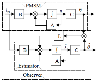
Figure 1 shows the proposed sensorless control scheme by using Luenberger observer.
Figure 1. Structure of the Luenberger observer
2.2 Back-EMF observer
A state representation in the (αβ) coordinates of the PMSM is modeled as [18]:
$\frac{d}{d t}\left[\begin{array}{c}{i_{s a}} \\ {i_{s \beta}}\end{array}\right]=\frac{1}{L_{d}}\left[\begin{array}{cc}{-R_{s}} & {-w\left(L_{d}-L_{q}\right)} \\ {w\left(L_{d}-L_{q}\right)} & {-R_{s}}\end{array}\right]\left[\begin{array}{c}{i_{s \alpha}} \\ {i_{s \beta}}\end{array}\right]$
$+\frac{1}{L_{d}}\left[\begin{array}{cc}{-1} & {0} \\ {0} & {-1}\end{array}\right]\left[\begin{array}{c}{e_{s \alpha}} \\ {e_{s \beta}}\end{array}\right]+\frac{1}{L_{d}}\left[\begin{array}{c}{v_{s \alpha}} \\ {v_{s \beta}}\end{array}\right]$ (9)
where $e_{s \alpha}, e_{s \beta}$ are the back Electro Motive Forces (EMF) in the (αβ) reference frame. They are defined as:
$\left[\begin{array}{c}{e_{s a}} \\ {e_{s \beta}}\end{array}\right]=\left[\left(L_{d}-L_{q}\right)\left(w i_{s d}-\frac{d i_{s q}}{d t}\right)+\phi w\right]\left[\begin{array}{c}{-\sin \theta} \\ {\cos \theta}\end{array}\right]$ (10)
Eq. (9) can be used to estimate $e_{s \alpha}, e_{s \beta}$ [19].
$\frac{d}{d t}\left[\begin{array}{c}{\hat{i}_{s \alpha}} \\ {\hat{e}_{s \alpha}}\end{array}\right]=\frac{1}{L_{d}}\left[\begin{array}{cc}{-R_{s}} & {-1} \\ {0} & {0}\end{array}\right]\left[\begin{array}{c}{\hat{i}_{s \alpha}} \\ {\hat{e}_{s \alpha}}\end{array}\right]+\left[\begin{array}{c}{k_{\alpha 1}} \\ {k_{\alpha 2}}\end{array}\right] \tilde{i}_{s \alpha}$ $+\frac{1}{L_{d}}\left[\begin{array}{l}{1} \\ {0}\end{array}\right]\left(v_{s \alpha}-\hat{w}\left(L_{d}-L_{q}\right) i_{s \beta}\right)$ $\frac{d}{d t}\left[\begin{array}{c}{\hat{i}_{s \beta}} \\ {\hat{e}_{s \beta}}\end{array}\right]=\frac{1}{L_{d}}\left[\begin{array}{cc}{-R_{s}} & {-1} \\ {0} & {0}\end{array}\right]\left[\begin{array}{c}{\hat{i}_{s \beta}} \\ {\hat{e}_{s \beta}}\end{array}\right]+\left[\begin{array}{c}{k_{\beta 1}} \\ {k_{\beta 2}}\end{array}\right] \tilde{i}_{s \beta}$ $+\frac{1}{L_{d}}\left[\begin{array}{l}{1} \\ {0}\end{array}\right]\left(v_{s \beta}+\hat{w}\left(L_{d}-L_{q}\right) i_{s \alpha}\right)$ (11)
where
$\left\{\begin{array}{l}{\tilde{i}_{s \alpha}=\hat{i}_{s \alpha}-i_{s \alpha}} \\ {\tilde{i}_{s \beta}=\hat{i}_{s \beta}-i_{s \beta}}\end{array}\right.$ (12)
A discretization of the linear and stationary continuous model is employed here [15]. The dynamics of the errors are:
$\frac{d}{d t}\left[\begin{array}{c}{\tilde{i}_{s \alpha}} \\ {\tilde{e}_{s \alpha}}\end{array}\right]=\left[\begin{array}{cc}{k_{\alpha 1}-\frac{R_{s}}{L}} & {-\frac{1}{L}}\end{array}\right]\left[\begin{array}{c}{\tilde{i}_{s \alpha}} \\ {\tilde{e}_{s \alpha}}\end{array}\right]$
$\frac{d}{d t}\left[\begin{array}{c}{\tilde{i}_{s \beta}} \\ {\tilde{c}_{s \beta}}\end{array}\right]=\left[\begin{array}{cc}{k_{\beta 1}-\frac{R_{s}}{L}} & {-\frac{1}{L}} \\ {k_{\beta 2}} & {0}\end{array}\right]\left[\begin{array}{c}{\tilde{i}_{s \beta}} \\ {\tilde{e}_{s \beta}}\end{array}\right]$ (13)
where $\widetilde{e}_{s a}=\hat{e}_{s a}-e_{s a}, \widetilde{e}_{s \beta}=\hat{e}_{s \beta}-e_{s \beta}$ and $k_{\alpha 1}, k_{\alpha 2}, k_{\beta 1} k_{\beta 2}$ are the observer gains determined by pole-placement.
Using the adaptive observer of (11), the estimated EEMF components (αβ) can be written as follows:
$\begin{aligned} \dot{e}_{s \alpha} &=-\omega e_{s \beta} \\ \dot{e}_{s \beta} &=\omega e_{s \alpha} \end{aligned}$ (14)
From (14) the adaptive observer can be written as:
$\begin{aligned} \dot{\hat{e}}_{s \alpha} &=-\hat{\omega} \hat{\hat{e}}_{s \beta}-G\left(\hat{\hat{e}}_{s \alpha}-\hat{e}_{s \alpha}\right) \\ \hat{\hat{e}}_{s \beta} &=-\hat{\omega} \hat{\hat{e}}_{s \alpha}-G\left(\hat{\hat{e}}_{s \beta}-\hat{e}_{s \beta}\right) \end{aligned}$ (15)
where G is a positive observer gain tuned with pole-placement technique. The error dynamics are given as:
$\begin{aligned} \dot{\tilde{\hat{e}}}_{_{s \alpha}} &=-\tilde{\omega} \hat{e}_{s \beta}-G \tilde{\hat{e}}_{s \alpha} \\ \dot{\tilde{\hat{e}}}_{s \beta} &=\tilde{\omega} \hat{e}_{s \alpha}-G \tilde{\hat{e}}_{s \beta} \end{aligned}$ (16)
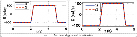
To evaluate the performances of the described methods, a set of simulations have been performed on a Matlab/Simulink. The current control algorithm is carried out every 100 μs, and the speed control loop is carried out every 1ms. In this structure, the PMSM is controlled by a PWM voltage source inverter using vector control strategy. The inverter switching frequency is 20 kHz, and the DC bus voltage is set at 200 V. The used PMSM parameters are listed in Table 1. The operating point is at high speed (the speed reference varies from -100 to +100 rad/s).
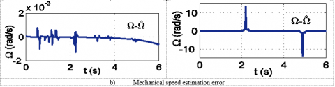
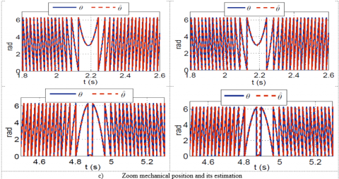
The results are displayed in Figures 2 and 3 respectively for the Luenberger and adaptive Back-EMF observers. Solid lines represent the actual mechanical speed, and dashed lines represent the estimation (Figures 2a and 3a). A Figure 2(b) and 3(b) shows the evolution of the errors on the speed respectively for both observers. The errors for the electrical position estimation are inferior to ± 0.3 rad (±0.1mechanical radian) both for observers. The results displayed in this test shows that Luenberger observer gives better results for position and speed estimations.
Table 1. PMSM characteristics
|
Symbol |
Symbol |
Parameter |
|
Ψm Ωn Tn Ld Lq Rs J F p Vn In |
Magnetic flux Nominal speed Nominal Load torque d-axis inductance q-axis inductance Stator resistance Moment of inertia Viscous friction Pole pairs Nominal voltage Nominal current |
0.153 Wb 314 rad/s 3.2 Nm 3.5 mH 4.5 mH 1.65 Ω 6.4 10-3 kg/m² 509 10 -3 Nm/rad 3 200 V 6 A |
Figure 2. Luenberger simulation results during a speed reversal test Figure 3. Back-EME simulation results during aspeed reversal test
In this section, mechanical sensor fault tolerant control mechanism including fault detection technique is presented. Fault tolerance is a fundamental requirement for dependable electric drives used in safety-critical applications or industrial processes where the very high costs of unplanned stops are unacceptable. There are two main FTC approaches: passive and active. In a passive FTC, one has to ensure that the control system works under all possible system operating scenarios that have been considered at the design stage, including potential component faults and/or failures. However, the system performance could be unacceptable in the presence of un-anticipated failures. Because a passive FTC has to maintain the system stability with various component failures, from the performance viewpoint, the designed controller has to be conservative. From typical relationships between the optimality and the robustness, it is very difficult for a passive FTCS to be optimal.
In this work, we propose the active FTC concept applied to a PMSM drive affected by a position/speed-sensor fault. The major steps involved in the FTC design are as follows:
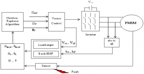
Figure 4 describes the proposed FTC architecture for PMSM drive at high speed, where the rotor position is obtained from a closed loop speed controller. In this section, we propose a voting algorithm based on based on Newton-Raphson method (NR) for the continuity of service by switching between two controllers than incorporate this position estimator into the closed loop controller. This algorithm is based on the comparison between an estimated signal obtained with NR approximation and the three inputs and on the voting algorithm.
Figure 4. The proposed sensor fault-tolerant control architecture
In general, the NR method for solving an equation:
$f(x)=0$ (17)
is based upon convergence, under suitable conditions [1, 2] of the sequence:
$y_{k+1}=y_{k}-\frac{y_{k}^{\prime}}{y_{k}^{\prime}} ;(k=0,1,2, \ldots)$ (18)
to a solution of (1), where k0 is an approximation solution, A details discussion of the method, together with many applications.
Extensions to systems of equations
$\left\{\begin{array}{l}{f_{1}\left(x_{1}, \ldots, x_{n}\right)=0} \\ {f_{m}\left(x_{1}, \ldots, x_{n}\right)=0}\end{array} \quad \text { or } f(X)=0\right.$ (19)
the Newton-Raphson method is a very efficient method in the search for the zero of a real function and its convergence is generally much faster.
Where $y_{k}^{\prime}$ and $y_{k}^{\prime \prime}$ are the first and second derivate of yk respectively. We find the approximate solution (X0) where the first derivative of this function will be zero. The presence of the first and second derivatives shows that this method is more suitable for continuous signals. A detailed discussion of the method, together with many applications, can be found in [20-21].
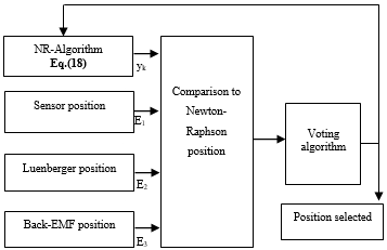
The proposed structure of the FTC for PMSM is shown in Figure 4. This structure is based on the use of a diagnostic module called fault detection and isolation (FDI) and a voting algorithm. In literature, many probabilistic voting algorithm techniques, such as, the likelihood, Euler, Newton-Raphson, are used, where each approach has its advantages and drawbacks. In this paper, the so-called Newton-Raphson based voting algorithm is suggested, since it’s allows to reconstruct the observed state without intensive calculus. The voting algorithm is designed to feedback to the controller the most accurate position information between the three inputs that are the sensor, the EMF or the Luenberger observer, as shown in Figure 5.
Figure 5. Voting algorithm based on Newton-Raphson approach
This algorithm is based on the comparison of the sensor position output, its estimation, either by Luenberger, and the Back-EMF method, with a fictitious input, obtained by the Newton-Raphson approximation, according to a sampling period, and a chosen threshold.
The following steps describe the algorithm used for the selection logic of the positions sensor or observers are drawn up, in case of position information loss which is as follows:
• If E1 < threshold, no defect is noticed, and consequently, the current sensing is adopted.
• If E1> threshold, a sensor fault is remarked. The estimation is then obtained via one of the two observers, presenting the weakest residue E2 or E3.
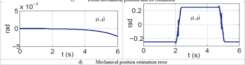
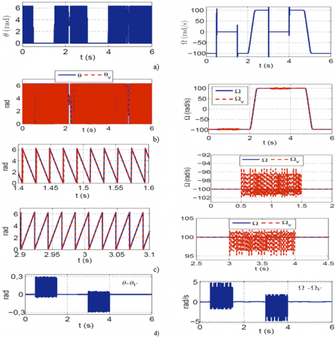
In general, the PMSM drive can be affected by failures in the battery (short-circuited cell), failures in the power converters (short-circuit or open-circuit of the power switches) [22], failures of the sensors (mechanical or electrical), or failures in the electrical machine [23-24]. To evaluate all this structure, we suppose that in the time range [0.5s - 1.5s] and [3s - 4s] associated to healthy operation we have a mechanical sensor failure (complete outage) at high speed as shown in figure 6. The simulation results obtained show clearly the effectiveness of the FTC scheme that occurs during the application of the fault by removing all defects thanks to the FTC strategy. In sensor faulty conditions, it is found that the observers have better performance for high speed. We see that the rotor mechanical voting speed (ΩV) or the rotor electrical voting position (θV) follow up the reference quickly and perfectly for the NR which confirms the robustness.
Figure 6. Simulation results in case of mechanical sensor failure during a speed reversal test with using the proposed FTC scheme
a) Faulted rotors position and speed
b) Actual and voting rotors position and speed
c) Position and speed-sensor zooms around faults at (-100 rad/s) and (+100 rad/s)
d) Position and speed voting errors
In this paper, we have investigated the possibility to implement a mechanical sensor fault-tolerant control for a PMSM drive system at high speed. The fault tolerant control is built with two virtual sensors, the Luenberger and adaptive back-EMF observers combined to a voting algorithm by using Newton-Raphson method. The simulation results show the robustness of the proposed control scheme, and confirm that the NR is more efficient. The controller has been evaluated under failure to the mechanical sensor (complete outage).
[1] Kisck, D.O., Chang, J.H., Kang, D.H., Kim, J.W., Anghel, D. (2010). Parameter identification of permanent-magnet synchrounous motors for sensorless control. Rev. Roum. Sci. Techn. – Électrotechn. et Énerg., 55(2): 132–142.
[2] Johnson, J.P., Ehsani, M., Guzelgunler, Y. (1999). Review of sensorless methods for brushless DC. In Conference Record IEEE Industry Applications Conference, pp. 143–150. http://doi.org/10.1109/IAS.1999.799944
[3] Holtz, J. (2006). Sensorless control of induction machines with or without signal injection. IEEE Transactions on Industry Electronics, 53(1): 7-30. http://dx.doi.org/10.1109/TIE.2005.862324
[4] Aydogmus, O., Sünter, S. (2012). Implementation of EKF based sensorless drive system using vector controlled PMSM fed by a matrix converter. Inter. Journal of Electrical Power & Energy Systems, 43(1): 736-743. http://dx.doi.org/10.1016/j.ijepes.2012.06.062
[5] Chen, Z., Tomita, M., Doki, S., Okuma, S. (2003). An extended electromotive force model for sensorless control of interior permanent magnet synchronous motors. IEEE Trans. Ind. Electron., 50(2): 288-295. http://dx.doi.org/10.1109/TIE.2003.809391
[6] Eom, W., Kang, I., Lee, J. (2008). Enhancement of the speed response of PMSM sensorless control using an improved adaptive sliding mode observer. IEEE International Conf. On Industrial Electronics IECON, Orlando, USA. http://dx.doi.org/10.1109/IECON.2008.4757950
[7] Diao, S., Diallo, D., Makni, Z., Marchand, C., Bisson, J.F. (2015). A differential algebraic estimator for sensorless permanent-magnet synchronous machine drive. IEEE Transactions on Energy Conversion, 30(1): 82-89. http://dx.doi.org/10.1109/TEC.2014.2331080
[8] Medjmadj, S., Diallo, D., Mostefai, M., Delpha, C., Arias, A. (2015). PMSM drive position estimation: contribution to the high-frequency injection voltage selection issue. IEEE Transactions on Energy Conversion, 30(1): 349-358. http://dx.doi.org/10.1109/TEC.2014.2354075
[9] Hagras, H. (2007). Type-2 FLCs: A new generation of fuzzy controllers. IEEE Computational Intelligence Magazine, 2(1): 30-43. https://doi.org/10.1109/mci.2007.357192
[10] Ye, S.C. (2018). A novel fuzzy flux sliding-mode observer for the sensorless speed and position tracking of PMSMs. Optick-Int. Journal for Light and Electron Optics, 171: 319-325. https://doi.org/10.1016/j.ijleo.2018.06.074
[11] Poulain, F., Praly, L., Ortega, R. (2008). An observer for PMSM with application to sensorless control. 47th IEEE Conference on Decision and Control, Cancun, Mexico.
[12] Campos-Delgado, D.U., Palacios, E., Espinoza-Trejo, D.R. (2008). Fault tolerant control in variable speed drives: A survey. IET Electric Power Applications, 2(2): 121-134. https://doi.org/10.1049/iet-epa:20070203
[13] Zhou, Y., Lin, X., Cheng, M. (2016). A fault-tolerant direct torque control for six-phase permanent magnet synchronous motor with arbitrary two opened phases based on modified variables. IEEE Trans. on Energy Conversion, 31(2): 549-556. http://dx.doi.org/10.1109/TEC.2015.2504376
[14] Bakhti, I., Chaouch, S., Makouf, A., Douadi, T. (2016). Robust sensorless sliding mode control with Luenberger observer design applied permanent magnet synchrounous motor. 5th International Conference on Systems and Control (ICSC), Marrakesh, Morocco, pp. 204–210. http://dx.doi.org/10.1109/ICoSC.2016.7507051
[15] Grellet, G., Clerc, G. (1996). Actionneurs éLectriques: Principes, Modèles, Commande. Collection Electrotechnique, Edition 2, Eyrolles, 491 pages.
[16] Jouili, M., Jarrayb, K., Koubaa, Y., Boussakc, M. (2012). Luenberger state observer for speed sensorless ISFOC induction motor drives. Electric Power Systems Research, 89: 139-147. https://doi.org/10.1016/j.epsr.2012.02.014
[17] Henwood, N., Malaize, J., Praly, L. (2012). A robust nonlinear Luenberger observer for the sensorless control of SM-PMSM: Rotor position and magnets flux estimation. 38th Annual Conference on IEEE Industrial Electronics Society, Montreal, QC, Canada, pp. 1625-1630. https://doi.org/10.1109/IECON.2012.6388732
[18] Akrad, A., Diallo, D., Hilairet, M. (2011). Design of a fault-tolerant controller based on observers for a PMSM drive. IEEE Trans. Ind. Electron., 58(4): 1416-1427. https://doi.org/10.1109/TIE.2010.2050756
[19] Ichikawa, S., Tomita, M., Doki, S., Okuma, S. (2001). Sensorless control of an interior permanent-magnet synchronous motor on the rotating coordinate using an extended electromotive force. In Proc. IEEE IECON, 3: 1667-1672. https://doi.org/10.1109/IECON.2001.975538
[20] Idema, R, Lahaye, D.J.P., Vuik, C. (2011). Repport 11-14. On the convergence of inexact Newton methods. Reports of the Department of Applied Mathematical Analysis. Delft University of Technology.
[21] Dembo, R.S., Eisenstat, S.C., Steihaug, T. (1982). Inexact Newton methods. SIAM J. Numer. Anal., 19(2): 400-408.
[22] Sun, D., He, Y. (2005). A modified direct torque control for PMSM under inverter fault. In Proc. Int. Conf. Elect. Mach. Syst., Nanjing, China, 3: 2473. https://doi.org/10.1109/ICEMS.2005.203019
[23] Espinoza-Taejo, D.R., Campos-Delgad, D.U. (2008). Active fault tolerant scheme for variable speed drives under actuator and sensor faults. 17h IEEE. Int. Conf. Control Applications, San Antonio, Texas, USA, pp. 474-479.
[24] Campos-Delgado, D.U., Martinez-Martinez, S., Zhou, K. (2005). Integrated fault tolerant scheme for a DC speed drive. IEEE/ASME Trans. Mechatronics, 10(4): 419-427. https://doi.org/10.1109/TMECH.2005.852494