Junhui Zheng* | Deyong Wang | Zexun Geng
OPEN ACCESS
Coal mine monitoring video image data is characterized by overall dark and blurry, low contrast, poor illumination, and a large amount of noise. The quality of the data directly affects the accuracy of the recognition algorithm, multi-scale decomposition method with noise suppression and structure protection is the core of the detail enhancement algorithm. The existing detail enhancement method based on L0 norm minimization only utilizes local structural information, and it is difficult to effectively filter the noise existing in the video data. Aiming at the existing problems, a coal mine monitoring data detail enhancement algorithm based on L0 norm and low rank analysis was proposed and achieved good results.
coal mine monitoring video, L0 norm, low rank analysis, enhancement algorithm
Coal mine video data is limited by the environment, so the images are blurred, the contrast is low, the illumination changes greatly, the noise is large, the features are weak, and the dimension is high, all of which bring difficulty to the recognition [1]. As the data source of coal mine miner behavior identification, the quality of coal mine monitoring data directly affects the accuracy of the identification algorithm [2]. Therefore, the pretreatment of coal mine monitoring data becomes an indispensable step of the behavior identification algorithm. In the coal mine monitoring data preprocessing method, the detail enhancement algorithm is a hot spot in the current research which can effectively improve the accuracy of monitoring data feature extraction [3-4]. Among them, the core problem of the detail enhancement algorithm is to design a structure-preserving data multi-scale representation method [5]. In recent decades, various algorithms with structure preserving ability have been successively proposed and achieved remarkable results [6]. The research goal in this direction is to enhance the inherent structural information of the data, to suppress the gradient inversion phenomenon and to compress the noise [7].
Although current researches have achieved some results in the detail enhancement method, the multi-scale representation method of structure preserving still faces many pending problems, such as: how to effectively extract the structural information within the data, how to compromise the representation ability of local structure and global structure, how to effectively deal with significant structural information when conducting multi-scale decomposition, and how to compress the occurrence of gradient inversion phenomenon and suppress and eliminate the noises [8].
In order to solve above problems, this paper organically combines the multi-scale decomposition based on non-local L0 norm model with the significant information extraction based on low rank analysis and proposes a coal mine monitoring data detail enhancement algorithm based on L0 norm and low rank analysis.
The core of the coal mine monitoring data detail enhancement algorithm is the multi-scale representation of data based on structure awareness, the decoupling of noise and structural information, and the detail enhancement of different scales on this basis [9]. In this paper, the coal mine monitoring data structure awareness multi-scale analysis is constructed by coupling the adaptive non-local L0 model, and the low-rank analysis model is used to decouple the noise and structural information, and then the Sigmoid function is introduced to implement the detail enhancement of different scales.
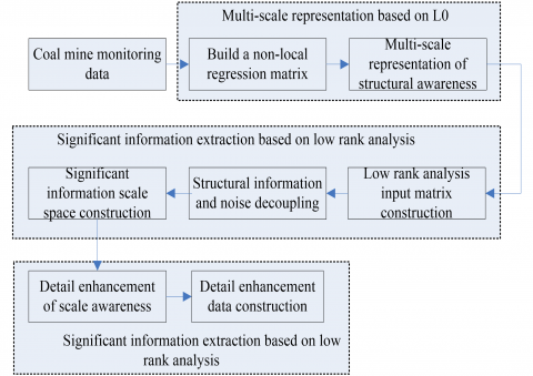
This paper presents a method for enhancing details of coal mine monitoring data based on L0 norm and low rank analysis. As shown in Figure 1, the proposed method consists of three major functional modules, respectively are: multi-scale representation based on L0 norm, the extraction of significant information based on low rank analysis and scale-related detail enhancement, mainly including 7 steps:
(1) Build a non-local regression matrix.
(2) Multi-scale representation of structural awareness.
(3) Low rank analysis input matrix construction.
(4) Structural information and noise decoupling.
(5) Significant information scale space construction.
(6) Detail enhancement of scale awareness.
(7) Detail enhancement data construction.
Figure 1. A flowchart of detail enhancement method for coal mine monitoring data based on L0 norm and low rank analysis
3.1 L0 norm minimization model
Proposed a global optimization algorithm based on the L0 paradigm and achieved the global optimization solution of the image by constraining the number of gradient modulus values [10]. Replaced the fidelity term L2 with L1 based on the L0 optimization algorithm.
The definition of the model based on L0 norm minimization is as follows:
$\underset{B(x,y)}{argmin}\underset{(x,y)}{\sum}(B(x,y)-L(x,y))^2+λ_1C(B(x,y))$ (1)
where, the first item $(B(x,y)-L(x,y))^2$ is the fidelity item, which ensures the consistency of structural information between the output smooth image $B(x,y)$ and the input image $L(x,y)$, $λ_1$ is the scale parameter which realizes the compromise between the fidelity item and the constraint item, $C(B(x,y))$ represents the L0 norm constraint item of the smooth image $B(x,y)$, its definition is as follows:
$C(B(x,y))$=# $\{ (x,y)||\bigtriangledown B(x,y)|\not=0 \}$ (2)
where, $\bigtriangledown$ represents a difference operator, # represents the non-zero number. The matrix representation of the formula is as follows:
$\underset{B}{argmin}||B-L||^2_2+λ_1||\bigtriangledown B||_0$ (3)
where, "$|| ||$" is the L2 norm. Since the L0 norm-based minimization model adopts constraints on the gradient terms, the model has a good structural awareness, but ignores the non-local structural information within the image. In addition, using this model to implement detail enhancement introduces a large number of gradient inversions at the boundary. In order to solve the above two major problems, this paper proposes to introduce non-local constraints to the L0 norm-based minimization model.
3.2 Non-local L0 norm minimization model
Introducing the non-local regression model to the L0 norm-based minimization model, the optimized model is defined as follows:
$\underset{B}{argmin}||B-L||^2_2+λ_1||\bigtriangledown B||_0+λ_2||WΦB||^2_2$ (4)
where, $||WΦB||^2_2$ is a non-local constraint item, W is non-local regression matrix, $Φ$ is the structural extraction matrix of image B, in this paper, the matrix $Φ$ is constructed by the gradient operators, $λ_2$ is a compromise parameter.
(1) Image block representation
in order to construct a non-local regression matrix W, a frame of image in the video needs to be partitioned. Normalize the image block $p_i$ with dimension $s×s$ :
$p_i=\frac{p_i-μ_i}{σ_i}$ (5)
where, $μ_i$ and $σ_i$ represent the mean and standard deviation of the image block $p_i$, respectively.
It is necessary to further structurally encode the image block $p_i$, in which the similarity measure between the pixel i and the pixel j of the image block center is defined as follows:
$f_{ij}=exp(-\frac{(i-j)^2}{2σ^2_2}), j \in p_i$ (6)
where i and j represent the spatial coordinates of the pixels, pixel j is in the image block, $c_i$ represents the gray level value of pixel i, $σ_1$ and $σ_2$ are the standard deviation of the spatial and luminance parameters of the bilateral filter. Through formula (6), we can get the similarity between all pixels in the image block and the center pixel i, and use this to construct the structure kernel representation $F_i \in \mathbb{R}^{s×s}$ of the image block i, s is the width of the extracted image block, the definition is as follows:
$F_i=\begin{bmatrix} f_{i1} & f_{i2} & \ldots & f_{i(s-1)} & f_{is}\\ \vdots & \vdots & \ddots & \vdots & \vdots\\ f_{i(s^2-s+1} & f_{i(s^2-s+2} & \ldots & f_{i(s^2-1} & f_{is^2}\\ \end{bmatrix}$ (7)
Similarity measure: based on the structural kernel representation information of the image block constructed above, the block matching method uses the similarity measure to achieve the search of image blocks with similar structures, and its core is the design of the similarity measure method between blocks, which is defined as follows
$ω_{ik}=exp(-\frac{|||F_i-F_k|^2_2}{2σ_3^2})$ (8)
where, $F_i$ and $F_k$ represent the structural representation kernel of the image block i and the image block k, respectively, $σ_3$ is the standard deviation of similarity measure, which is used to control the sensitivity of the structural similarity measure. Based on above similarity measure formula, within the search range, the block matching algorithm obtains similarity weight satisfying $ω_{ik}≥0.98$ or the image blocks are located in the top 30 of similarity, then construct the non-local constraint matrix with the matched image blocks.
Construction of the non-local regression matrix W: based on the matching image blocks obtained by the block matching algorithm, a non-local regression matrix of a certain frame image in the coal mine monitoring video is constructed, and the similarity weight of the image block i and the image block k is $ω_{ik}$ , the constructed non-local regression coefficient matrix W is defined as follows:
$W(i,k)=\begin{cases} -ω_{ik} & \text{if patch k is similar to patch i}\\ 1 & \text{if } i=k\\ 0 & \text{otherwise } \end{cases}$ (9)
3.3 Optimization solution of non-local l0 norm minimization model
After the non-local constraint matrix W is determined, formula (4) contains only one variable output image B, but since formula (4) contains the L0 constraint term $||\bigtriangledown B||_0$, so the optimization function is non-convex, by introducing two intermediate variables $T_x$ and $T_y$ to replace the gradients $\frac{∂B}{∂X}$ and $\frac{∂B}{∂y}$ of the output image B in x and y direction, the formula (4) is rewritten as follows:
$\underset{B,T_x,T_y}{argmin}||B-L||^2_2+β(||∂_xB-T_x||^2_2+||∂_yB-T_y||^2_2)+λ_1|||T_x|+|T_y|||_0+λ_2||WΦB||^2_2=\underset{B,T_x,T_y}{argmin}||B-L||^2_2+β(||∂_xB-T_x||^2_2+||∂_yB-T_y||^2_2)+λ_1|||T_x|+|T_y|||_0+λ_2||WΦB||^2_2$ (10)
where, $c=WΦ$, parameter $β$ controls the consistency between the intermediate variables $T_x$, $T_y$ and the gradients $\frac{∂B}{∂X}$ and $\frac{∂B}{∂y}$ when parameter $β$ is large enough, the formula (10) is equivalent to formula (4).
By expressing the gradient operators $∂_X$ and $∂_y$ in x and y directions into a matrix form, the formula (10) can be rewritten as:
$\underset{B,T_x,T_y}{argmin}||B-L||^2_2+β(||Φ_xB-T_x||^2_2+||Φ_yB-T_y||^2_2)+λ_1|||T_x|+|T_y|||_0+λ_2||CB||^2_2$ (11)
Formula (11) can be solved by using the alternating iterative method to obtain variables B, $T_x$ and $T_y$, during each iterative solution, one or two variables are fixed to solve the remaining variables. The optimization function solution steps are divided into two sub-problems: smooth image B sub-problem and intermediate variables $T_x$ and $T_y$ sub-problem. The detailed optimization solution is as follows:
The sub-problem of smooth image B: fix intermediate variables $T_x$ and $T_y$, ignoring the related items without variable B in formula (11), the optimization function can be simplified as:
$\underset{B}{argmin}||B-L||^2_2+β(||Φ_xB-T_x||^2_2+||Φ_yB-T_y||^2_2)+λ_2||CB||^2_2$ (12)
Calculate the derivative of B using formula (12), set the derivative equal to 0, then we can get the expression for B as:
$\frac{∂||B-L||^2_2+β(||Φ_xB-T_x||^2_2+||Φ_yB-T_y||^2_2+λ_2||CB||^2_2}{∂B}=0$
$\Rightarrow (1+βΦ_x^TΦ_x+βΦ_y^TΦ_y+λ_2C^TC)B=βΦ_x^TT_x+βΦ_y^TT_y+L$ (13)
where, "1" represents a unit matrix. The coefficient matrix of the formula $(1+βΦ_x^TΦ_x+βΦ_y^TΦ_y+λ_2C^TC)$ is symmetric, sparse, and positive definite. Therefore, a preconditioned conjugate gradient method can be used to achieve a rapid reconstruction of a smooth image. In the algorithm implementation, the MATLAB pcg function is used to solve the formula (13).
The sub-problem of intermediate variables $T_x$ and $T_y$: Fix variable B in this iteration, formula (11) can be simplified as:
$\underset{T_x,T_y}{argmin}β(||Φ_xB-T_x||^2_2+||Φ_yB-T_y||^2_2)+λ_1|||T_x|+|T_y|||_0$ (14)
Since $|||T_x|+|T_y|||_0$ would return the non-zero number of $|T_x|+|T_y|$ , therefore, the optimization function can be implemented by a pixel-by-pixel optimization solution, and formula (14) can be rewritten as:
$\sum_i\underset{T^i_x,T^i_y}{min}β((∂_xB_i-T_x^i)^2+(∂_yB_i-T_y^i)^2)+λ_1(|T_x^i|+|T_y^i|)^0$ (15)
When $|T_x^i |+|T_y^i |\not=0$ , $(|T_x^i|+|T_y^i|)^0$ is 1, otherwise it is 0. For pixel i, the optimization function is as follows:
$\underset{T^i_x,T^i_y}{min}β((∂_xB_i-T_x^i)^2+(∂_yB_i-T_y^i)^2)+\frac{λ_1}{β}(|T_x^i|+|T_y^i|)^0$ (16)
The optimal solution of formula (16) is:
\( (T^i_x,T^i_y)=\begin{cases}(0,0) & ((∂_xB_i)^2+((∂_yB_i)^2≤\frac{λ_1}{β} \\ (∂_xB_i,∂_yB_i) & \text{otherwise} \end{cases} \) (17)
Through the iterative solution of the above two sub-problems, the optimization function eventually converges to the optimal solution and achieves smooth output of the structurally protected image.
The main advantages of introducing the low-rank analysis model include: (1) It simplifies the selection of scaling parameters $λ_1$ and $λ_2$; (2) The low-rank part of low-rank analysis represents the significant information in similar scale space, enabling decoupling of structural information and noise, thus improving the noise robustness of the algorithm.
Low-rank analysis model: from the matrix decomposition point of view, the matrix C can be decomposed into three parts: the low-rank part R, the sparse part S, and the noise part G. Therefore, the low-rank analysis model is defined as follows:
$C=R+S+G$, s.t. $rank(R)≤r,card(S)≤c$ (18)
Parameters r and c respectively represent rank constraint and cardinality constraint. For a given dense matrix $C \in \mathbb{R}^{m×n}$ and a bilateral random projection with rank r, the low-rank part R of the matrix C with rank r is expressed as:
$R=Y_1(A^T_2Y_1)^{-1}Y^T_2$ (19)
$Y_1=CA_1$, $Y_2=C^TA_2$, $A_1 \in \mathbb{R}^{n×r}$ and A_2 \in \mathbb{R}^{m×r}$. When the singular value of the matrix C decays slowly, the solution performance of formula (0-19) will drop rapidly. By introducing a power method, matrix C can be replaced by $\tilde{C}=(CC^T)^qC$ to accelerate low-rank approximation and improve precision, and q is a power iteration parameter. Therefore, the bilateral random projections BRP of the matrix C are $Y_1=\tilde{C}A_1$ , $Y_2=\tilde{C}A_2$. The low-rank approximation matrix $\tilde{R}$ of the matrix C is defined as:
$\tilde{R}=Y_1(A^T_2Y_1)^{-1}Y^T_2$ (20)
By performing QR decomposition on matrix $Y_1$ and matrix $Y_2$ , a low rank matrix R of matrix C can be obtained, defined as follows:
$R=(\tilde{R})^{\frac{1}{2q+1}}=Q_1[R_1(A^T_2Y_1)^{-1}R^T_2]Q^T_2$ (21)
Based on the obtained low rank part, the sparse part S of the matrix B is defined as:
$S=Υ_Ω(C-R)$ (22)
The function $Υ_Ω$ extracts c largest terms of a non-zero subset Ω within the matrix $C-R$, the noise part of the matrix C is G=C-R-S.
Scale-related significant information extraction: in order to be able to extract significant structural information within a similar-scale smooth image group, the obtained smooth images under the dense-scale parameters $λ_1$ and $λ_2$ need to be grouped, and then a low-rank analysis model is used to perform low-rank analysis on each image group, and extract the low-rank part as the significant structural information of the image group.
L represents an input image, B(t) represents a smooth image with a scale of $t=(λ_1^t,λ_2^t)$. Assume that each frame image of the coal mine monitoring data is represented as $u×ν$ smooth images, and the smooth images of this layer are divided into v groups, and each group contains u images. For each group of images, it is assumed that the related scale parameter sequence is an ascending sequence $[t_1^v,t_2^v,...,t_u^v]$, in which the ascending step length is fixed and the numerical value is small. Superscript k represents the group index, and the subscript represents the intra-group image index, so the intra-group images have similar scale values. For each image group, input image L is added to each image group, then by (v+1) images we can construct low rank analysis model’s input matrix $B^v=[L,B(t^v_1),...,B(t^v_u)]$. In order to extract the low-rank structural information of scale awareness, a large number of scale parameters are needed to obtain enough smooth images. The smooth images have similar scale parameters and high correlation, when the ascending step length is fixed, the scale awareness significant structural information extraction model only needs to determine the maximum value of the scale parameter $t=(λ_1^t,λ_2^t)$. At the same time, the scale parameter sequence will be evenly distributed into v groups and each group contain u images. Therefore, the problem of determining the maximum value of the scale parameter is converted into a problem of determining parameters u and v. Through the transformation of parameter problems, the selection problem of parameters $t=(λ_1^t,λ_2^t)$ is simplified to some extent.
A significant structural information extraction model based on layer low-rank analysis model is given above, for a given low-rank analysis input matrix $B^v$, a low-rank analysis model is used to extract the low-rank part $R^v$ of the image matrix, and then extract the first column’s data $R^{v,1}$ of the matrix $R^v$ as the significant information of this image group. For the noisy input image, the layer-based low-rank analysis model can extract the inherent significant structural information in the images and remove the noise at the same time. Therefore, the layer-based low-rank analysis model can inherently achieve the decoupling of noise and significant structural information. By performing low-rank analysis on each group of images, v significant structural information $\{R^{1,1},R^{2,1},...,R^{v,1}\}$ can be obtained. Since each group of images is related to a different scale sequence, a scale space can be constructed for the image by extracting v significant structural information.
Based on the constructed significant information multi-scale space, the high- and low-frequency information of one frame of data in the coal mine monitoring video has been separated into $\{D^1,D^2,…,R^ν\}$, in which $\{D^1,D^2,…,D^{ν-1)}\}$ is high-frequency detail information, and the frequency decreases with the increase of the superscript value. $R^v$ is low-frequency base layer information, including the main energy of a frame of data. Image detail enhancement is achieved by maintaining low frequency information and amplifying high frequency information. In order to prevent excessive value increase when enhancing the high details, the Sigmoid function is used to implement the detail enhancement. The Sigmoid function is defined as follows:
$\varphi(k,D^i)=\frac{1}{1+exp(-kD^i)}$ (23)
Di represents the i-th high-frequency detail information. Parameter k controls the steepness or flatness of the Sigmoid function curve. The transformed i -th high frequency detail information is translated and scaled. The translation function is defined as follows:
$shift=\varphi(k,D^i)-0.5$ (24)
The scaling function is defined as follows:
$D^i(k)=shift×\frac{0.5}{\varphi(k,0.5)-0.5}$ (25)
Formula (25) gives the basic processing method of detail information enhancement. In order to avoid the occurrence of gradient inversion at the boundary in the process of detail enhancement, different enhancement parameters $k$ need to be used for detail information with different frequencies. The proposed detail enhancement method is defined as follows:
$E=R^v+\sum^{v-1}_i=1D^i(k^i)$ (26)
where, E is the output image after detail enhancement, the enhancement parameter $k_i$ is set to be a geometric progression. According to the result of the evaluation index, the statistical analysis determines that $k_i$ is 25, and the common ratio is 0.85.
This section compares and analyzes the proposed algorithm and two representative algorithms. The comparison algorithms include L0-based method (L0) and bilateral filter-based method (BLF). The experimental comparison section (1) analyzes the choice of parameters, and (2) gives experimental results under Gaussian noise pollution with different decibel.
6.1 Parameter selection
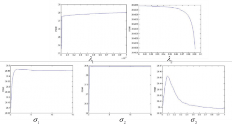
The algorithm proposed in this paper contains six parameters $(λ_1,λ_2,β,σ_1,σ_2,σ_3)$, for the detail-enhanced monitoring data, peak signal-to-noise ratio (PSNR) and mean structural similarity (MSSIM) are used to evaluate each test value of the parameter. For each test value, statistical values under all test images were averaged to construct an evaluation curve.
Parameter $λ_1$: As can be seen from Figure 2, if the value of $λ_1$ is too small, the instability of the algorithm will increase, resulting in too low PSNR statistics. As the value of $λ_1$ increases, the PSNR will gradually improve. When $λ_1=1.1e^{-4}$, better statistics of the evaluation indicators can be obtained.
Parameter $λ_2$: As can be seen from Figure 2, when $λ_2 \in [1.7e^{-3},1.2e^{-2}]$ , a better statistical value of the evaluation index can be obtained. Therefore, in the comparison experiment, parameter $λ_2$ is set to $4.3e^{-3}$ .
Figure 2. Parameter statistical curve
Parameter β : parameter β is set as β=$λ_1$ , and the parameter β is doubled each time as the number of iterations of the optimization function increases.
Parameters $σ_1$, $σ_2$ and $σ_3$: parameters $σ_1$, $σ_2$ control the structural sensitivity of the bilateral filtering kernel function of the image block, which directly affect the candidate non-local image block selection. As can be seen from Figure 3-2, when $σ_1=9$ and $σ_2=8.4$ , the evaluation indicators reach a steady state. When $σ_3=0.1$ , evaluation index reaches an optimal value. Therefore, in the comparison test, parameter $σ_3$ was set to 0.1.
6.2 Noise image experimental results and analysis
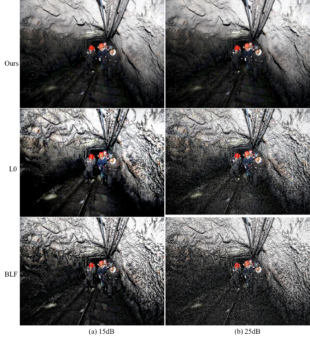
Figure 3 shows the comparison of the detail enhancement effects under 15dB and 25dB Gaussian noise disturbance conditions. Table 1 lists the corresponding PSNR and MSSIM evaluation index statistics. It can be seen from Table 1, that with the increase of noise intensity, the two evaluation indicators proposed in this paper have a slower rate of decline than the comparison method. At the same time, the proposed method has the optimal statistical value of the evaluation indicators, which proves that the noise and structural information decoupling model based on low rank analysis has good noise suppression effect. In addition, as can be seen from Figure 3, the algorithm of this paper has less noise in the detail enhancement of the noise image, at the same time the suppressed noise is being amplified, it effectively enhances the inherent details of the image. While the two algorithms BLF and L0 were enhancing the detail information, the noise data was also amplified, resulting the enhanced image containing a lot of noise, which seriously affects the visual effects and feature extraction.
Figure 3. Comparison of detail enhancement effects of 15dB and 25dB gaussian noise pollution images
Table 1. 15dB to 25dB Gaussian noise pollution detail enhanced image PSNR and MSSIM statistic
|
algorithms |
Ours |
L0 |
BLF |
|||
|
evaluation indicators |
PSNR |
MSSIM |
PSNR |
MSSIM |
PSNR |
MSSIM |
|
15dB |
27.89 |
0.70 |
16.02 |
0.26 |
15.03 |
0.24 |
|
25dB |
27.48 |
0.68 |
14.99 |
0.34 |
14.43 |
0.47 |
This paper proposes a method based on L0 norm and low rank analysis to enhance the details of coal mine monitoring data, by introducing non-local similarity constraint into the L0 norm optimization model, it makes the proposed L0 minimization model have local and non-local features, thus improving the model's structure awareness ability and multi-scale representation accuracy. Then, the scale-awareness structural information extraction algorithm based on low rank analysis is used to achieve the decoupling of noise and structural information of the proposed algorithm in a self-learning way, which greatly suppresses the noise from being amplified. A large number of experiments have proved that this algorithm has good anti-noise performance and detail enhancement ability.
This work is supported by the science and technology plan project of Henan province in 2017. (NO. 172102210118).
[1] Hua G, Jiang DH. (2014). A new method of image denoising for underground coal mine based on the visual characteristics. Journal of Applied Mathematics 4: 7-7. http://dx.doi.org/10.1155/2014/362716
[2] Wang L, Gu T, Tao X. (2012). A hierarchical approach to real-time activity recognition in body sensor networks. Pervasive and Mobile Computing 8(1): 115-130. https://doi.org/10.1016/j.pmcj.2010.12.001
[3] Carlsson S, Sullivan J. (2001). Action recognition by shape matching to key frames. Computer Engineering and Applications 47(2): 1-8.
[4] Matikainen P, Hebert M, Sukthankar R. (2010). Representing pairwise spatial and temporal relations for action recognition. European Conference on Computer Vision. Springer-Verlag, pp. 508-521. https://doi.org/10.1007/978-3-642-15549-9_37
[5] Matikainen P, Hebert M, Sukthankar R. (2009). Trajectons: Action recognition through the motion analysis of tracked features. IEEE, International Conference on Computer Vision Workshops, pp. 514-521. https://doi.org/10.1109/ICCVW.2009.5457659
[6] Turaga P, Chellappa R, Subrahmanian VS. (2008). Machine recognition of human activities: A survey. IEEE Transactions on Circuits and Systems for Video Technology 18(11): 1473-1488. https://doi.org/10.1109/tcsvt.2008.2005594
[7] Ryoo MS, Aggarwal JK. (2009). Spatio-temporal relationship match: Video structure comparison for recognition of complex human activities. Proceedings, pp. 1593-1600. https://doi.org/10.1109/ICCV.2009.5459361
[8] Jiang Z, Lin Z, Davis LS. (2010). A tree-based approach to integrated action localization, recognition and segmentation. European Conference on Computer Vision. Springer, Berlin, Heidelberg, pp. 114-127. https://doi.org/10.1007/978-3-642-35749-7_9
[9] Hu Y, Cao L, Lv F. (2009). Action detection in complex scenes with spatial and temporal ambiguities. IEEE, International Conference on Computer Vision, pp. 128-135. https://doi.org/10.1109/ICCV.2009.5459153
[10] Stauffer C, Grimson WEL. (2000). Learning patterns of activity using real-time tracking. IEEE Transactions on Pattern Analysis & Machine Intelligence 22(8): 747-757. https://doi.org/10.1109/34.868677
[11] Gorelick L, Blank M, Shechtman E. (2007). Actions as space-time shapes. IEEE Transactions on Pattern Analysis and Machine Intelligence 29(12): 2247-2253. https://doi.org/10.1109/ICCV.2005.28