Qian Guo | Chun Yang | Shaoqing Tian*
© 2020 IIETA. This article is published by IIETA and is licensed under the CC BY 4.0 license (http://creativecommons.org/licenses/by/4.0/).
OPEN ACCESS
The boom of e-commerce platforms (ECPs) has created a massive amount of data on user behaviors. To realize precision marketing, the ECPs must mine out the effective information from the massive data, and predict the purchase intention of their users. Therefore, this paper attempts to design an effective prediction model of purchase intention among ECP users. Firstly, feature engineering, coupled with big data analysis, was performed to identify the features that directly bear on the purchase intention of ECP users. Drawing on these features, two prediction models were established based on linear regression (LR) and extreme gradient boosting (XGBoost), respectively. The XGBoost model was found to be more effective through experiment on ECP users using cellphones. Finally, the prediction effects of the XGBoost-based prediction model were verified through an experiment on Epinions Trust Network Dataset. The research results provide new insights into user behaviors on ECPs.
big data analysis, purchase intention, feature engineering, e-commerce platform (ECP), extreme gradient boosting (XGBoost)
The rise of e-commerce has reshaped our consumption mode. Online shopping is siphoning a growing number of consumers from physical stores. The various behaviors of e-commerce platform (ECP) users, namely, order placement and payment, have generated a massive amount of data, which can be processed through data mining and machine learning. However, the e-commerce data are highly redundant, as users often browse through many unnecessary items on ECPs. To improve consumer stickiness, it is imperative to help ECP users find the items they need quickly.
At present, ECPs generally adopt three marketing strategies: issuing store or platform coupons during promotional activities, recommending a user for low-price items similar to those he/she added to the shopping cart, and referring a user to the items relevant to his/her search history. The three strategies are all ground on search or recommendation algorithms. Nevertheless, there is not yet an algorithm that effectively predicts the purchase intention of ECP users.
To make up for the gap, this paper develops a prediction model of purchase intention among users on an ECP. Specifically, the key features affecting the purchase intention of the users were extracted through feature engineering and big data analysis, and used to establish two prediction models based on linear regression (LR) and extreme gradient boosting (XGBoost), respectively. Next, the prediction effects of the two models on ECP users using cellphones were compared, and the XGBoost-based model was found to be the better one. Finally, the prediction effects of the XGBoost-based prediction model were verified through an experiment on Epinions Trust Network Dataset.
2.1 Data analysis
Data analysis has been widely used to predict the purchase intention of ECP users. Azad et al. [1] studied the main factors affecting the consumer loyalty and repeat purchase rate of Yahoo users. Zhu et al. [2] predicted the purchase intention of consumers by analyzing their behavior data, and examined the features of consumers who intend to make repeat purchase. Lucero [3] explored the relationship between influencing factors of group purchase and individual purchase on Amazon, revealing that ECP users prefer to purchase items with more comments and less restrictions on use.
The data analysis of ECP users is still in the exploratory stage. Most of the relevant studies focus on the application and optimization of algorithms. There is little report on the behavioral features of ECP users.
2.2 Recommendation algorithms
Recommendation algorithms [4] are another common method to predict the purchase intention of ECP users. Based on various social tags, Yuan et al. [5] designed a collaborative filtering (CF) recommendation algorithm for Sina Weibo users. Nanopoulos et al. [6] classified songs by social tags, and proved that the classification based on social tags is more accurate than that based on texts and other data sources. To make accurate recommendations, Salter and Antonopoulos [7] combined tag ranking and content-based filtering to calculate the tag relevance of film-related elements.
Punj [8] discussed the behavioral features of online book purchases, and proposed a collaborative recommendation algorithm to find users with similar behavior to the benchmark user. Focusing on online course recommendation, Lu et al. [9] searched for item sets related to content through item-based collaborative filtering, filtered the item sets by sequential pattern mining, and combined the two methods to recommend potentially useful courses to online learners. Ahmad et al. [10] recognized the correspondence between user actions and responses like page forwarding, and collected the data on shopping behavior through weblog analysis. Sun and Bin [11] extracted nine features from the poster, reader and content of Sina Weibo, and established a user behavior prediction model based on logical regression.
With the aid of radial basis function (RBF) neural network (NN), Lin et al. [12] designed a precision marketing strategy for telecom companies through the following steps: firstly, the key elements of clusters were selected through factor analysis; next, the cluster centers were identified by nearest neighbor clustering, and adjusted by k-means clustering (KMC); after that, the center of the RBF-NN was determined; finally, a consumer segmentation model was developed to describe the behavioral features of different users and make precise recommendations to each user. Martin and Herrero [13] improved the decision tree algorithm, and verified the effectiveness of the improved algorithm in predicting purchase behaviors.
To sum up, recommendation algorithms can indeed improve the prediction accuracy of purchase intention among ECP users, but face prominent defects like data sparsity, cold start and lack of scalability.
In the age of big data, data features are more important than prediction algorithms to the forecast of purchase intention. Hence, it is necessary to extract and screen out the typical features from the original data through feature engineering, and apply them to enhance the accuracy of prediction algorithms.
3.1 Problem description
Our problem aims to predict the purchase intention of users on an ECP in the next 5 days. Predicting whether a user will purchase a type of items was considered as a binary classification problem. If a user makes the purchase, he/she was tagged positive; if the user does not make the purchase, he/she was tagged negative.
In theory, the positive samples and negative samples should add up to all the users of the ECP, and the sample space should cover all the historical data of these users. In real-world scenarios, however, the purchase behavior in the next 5 days is not affected by the behavioral data of each and every user.
Therefore, this paper selects the active users in the 5 days before the forecast date as the samples, and extracted the features of the sample space from the user behavioral data in the 15 days before the forecast date. The interval between the same behavior in the training set and the test set was set to 5 days. Hence, the training and test sets were collected from 25 days.
Table 1. User information
|
Field name |
Meaning |
Data type |
|
User_id |
User ID |
String |
|
User_age |
Age group |
Enum; 6 age groups |
|
User_sex |
Gender |
Boolean |
|
Reg_date |
Registration date |
String |
|
User_level |
Level |
Enum |
|
Field name |
Explanation |
Data type |
|
User_id |
User ID |
String |
|
Item_id |
Item number |
Int |
|
Request_date |
Behavior date |
Date |
|
Request_time |
Behavior time |
Time |
|
Cate |
Category ID |
Int |
|
Brand |
Brand ID |
Int |
|
User_id |
Item_id |
Request_date |
Request_time |
Behavior |
Cate |
Brand |
|
cu_723b081 |
41 |
2019.7.3 |
13:31:26 |
click |
671 |
33 |
|
cu_723b081 |
41 |
2019.7.3 |
13:39:02 |
click |
671 |
33 |
|
cu_723b081 |
121 |
2019.7.6 |
20:17:33 |
click |
671 |
39 |
|
cu_723b081 |
121 |
2019.7.6 |
20:17:56 |
browse |
671 |
39 |
|
cu_723b081 |
315 |
2019.7.7 |
18:08:19 |
cart_add |
4287 |
66 |
|
cu_7a3e765 |
751 |
2019.7.4 |
11:22:18 |
click |
782 |
502 |
|
cu_7a3e765 |
751 |
2019.7.4 |
11:26:25 |
click |
782 |
502 |
|
cu_7a3e765 |
751 |
2019.7.4 |
12:39:38 |
click |
782 |
502 |
|
cu_7a3e765 |
352 |
2019.7.5 |
22:17:19 |
click |
93 |
609 |
|
cu_7a3e765 |
352 |
2019.7.5 |
22:37:56 |
order |
93 |
609 |
|
cu_7a3e765 |
57 |
2019.7.6 |
19:22:21 |
click |
802 |
772 |
|
cu_7a3e765 |
57 |
2019.7.6 |
19:28:22 |
click |
802 |
772 |
|
cu_81af3b1 |
323 |
2019.7.3 |
16:22:25 |
click |
872 |
111 |
|
cu_81af3b1 |
323 |
2019.7.3 |
16:27:22 |
browse |
872 |
111 |
|
cu_81af3b1 |
323 |
2019.7.3 |
16:28:25 |
order |
872 |
111 |
|
cu_81af3b1 |
421 |
2019.7.3 |
16:37:21 |
click |
332 |
1126 |
|
cu_81af3b1 |
421 |
2019.7.3 |
16:38:04 |
browse |
332 |
1126 |
|
cu_81af3b1 |
421 |
2019.7.3 |
16:39:22 |
cart_add |
332 |
1126 |
|
cu_81af3b1 |
421 |
2019.7.3 |
16:42:51 |
cart_del |
332 |
1126 |
|
cu_81af3b1 |
577 |
2019.7.4 |
10:01:04 |
click |
188 |
732 |
|
cu_81af3b1 |
577 |
2019.7.4 |
10:31:21 |
browse |
188 |
732 |
|
cu_81af3b1 |
577 |
2019.7.4 |
10:32:09 |
order |
188 |
732 |
As shown in Table 2, an ECP user has 6 different behaviors for an item, including browse, add to cart (cart_add), delete from cart (cart_del), order, follow, and click. Every behavior of the user for an item generates a behavior record. Table 3 displays the behavior data of three users. The behaviors of each user were sorted by behavior time.
In Table 3, the first line means user cu_723b081 clicked on item #41 in category 671# at 13:31:26 on June 3, 2019. The user operated over three items in two categories over 5 days. On this basis, the behavioral features of the user can be obtained through big data analysis, and used to predict whether the user will make a purchase in the next 5 days.
Considering the sheer number (10,725) and fast growth (3,500/day) of categories on the ECP, a resource strain will definitely appear if all the data in every category is analyzed. Therefore, the user behavioral data in one category, i.e. the users who have operated on cellphones, were selected for analysis.
In principle, all the historical data should be adopted for further analysis. However, the user behaviors in the next 5 days have little to do with those occurring half a year or one year ago. Hence, only a part of historical data was subjected to feature engineering.
3.2 Big data-based feature extraction
To extract the key features, statistical analysis was performed based on one or more information points. Judging by the data graph, the authors evaluated if a feature is meaningful or meaningless, and mined out new features.
Through big data analysis, the extracted features were divided into statistical features, category features, interval features, browsing features and calculation features.
(1) Statistical features
The statistical features include basic information, statistics on the six behaviors in each interval, the number of items operated in each interval, and the number of brands operated in each interval.
(2) Category features
The category features include the number of days that a category is operated, the number of days that a category is operated more frequently than others, the number of days that a category is operated earlier than others, and the maximum number of days that a category is operated continuously.
(3) Interval features
The interval features include the interval from the first browse to the day before the forecast date, the interval from the registration date to the forecast date, and the interval from the first order to the last order.
(4) Browsing features
The browsing features include the fractional addition of browsing depth in each interval, and the direct addition of browsing depth in each interval.
(5) Calculation features
The calculation features include ratio features, addition features, multiplication features and reduction features. Specifically, a ratio feature is quotient of the corresponding statistical feature and interval; an addition feature is the sum of normalized times of the six behaviors; a multiplication feature is the product between the number of active days and that of active behaviors; a reduction feature is the difference between the corresponding statistical features before and after an interval. The reduction feature can be described as:
$F(u, v)=\sum f(u, v)=\sum\left[v \times \log \left(1+\frac{1}{u+1}\right)\right]$ (1)
where, $\log (1+1 / u+1)$ is reduction function; v is the number of user behaviors on the current day; u is the interval between the current day and the day before the forecast date.
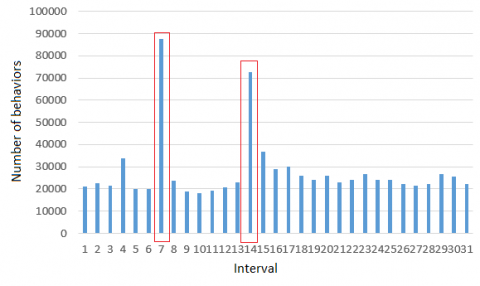
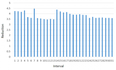
If a user browses an item 10 times on the day before the forecast date, and 10 times on the fifth day before the forecast date, then the F value of the former date must be greater than that on the latter date. In other words, the behavior closer to the forecast date was assigned a relatively high weight.
Figure 1 compares the statistical features of user behaviors before and after implementing the reduction function.
(a) Before reduction
(b) After reduction
Figure 1. Statistical features of user behaviors before and after implementing the reduction function
As shown in Figure 1, the number of behaviors had the same weight on each day, before the reduction function was implemented. After the reduction, the F value decreased with the increase of the interval, which reflects the negative correlation between the interval length and the importance of the number of behaviors.
The ten most and least important user behaviors were extracted through big data analysis, and listed in Tables 4 and 5, respectively.
Table 4. The ten most important user behaviors
|
Symbol |
Meaning |
|
f1 |
Number of clicks in 3 days |
|
f2 |
Number of items browsed in 3 days |
|
f3 |
Number of brands browsed in 3 days |
|
f4 |
Number of active days out of 3 days |
|
f5 |
Number of active hours out of 3 days |
|
f6 |
Interval from the first browse to the forecast date |
|
f7 |
Ratio of the number of browses in 3 days to the number of clikcss in 3 days |
|
f8 |
Additional user behaviors in 15 days |
|
f9 |
Product between the number of active days out of 3 days multiplied by number of user behaviors |
|
f10 |
Reduction in the number of clicks in 15 days |
|
Symbol |
Meaning |
|
f1 |
Number of browses in 15 days |
|
f2 |
Number of items browsed in 15 days |
|
f3 |
Number of brands browsed in 15 days |
|
f4 |
Number of active days out of 15 days |
|
f5 |
Number of active hours out of 15 days |
|
f6 |
Ratio of the number of clicks in 15 days to the number of browses in 15 days |
|
f7 |
Ratio of the number of browses in 3 days to the number of browses in 15 days |
|
f8 |
Mean daily number of behaviors in 15 days |
|
f9 |
Product between the number of clicks in 3 days and 3 |
|
f10 |
Product between the number of follows in 15 days and 15 |
4.1 LR-based prediction model
The LR [14] is a binary classification model that maps the results of linear functions to sigmoid functions. The LR prediction function can be expressed as:
$f_{\theta}(x)=1 / 1+e^{-\theta T_{x}}$ (2)
where, $f_{\theta}(x) \in(-1,1)$ is the predicted purchase probability; $\theta$ is the regression parameter.
If $f_{\theta}(x)$ is greater than or equal to 0.5, the target user is expected to make a purchase; otherwise, the target user is not expected to make any purchase.
The probability of sample generation can be expressed as:
$p(\mathrm{y} | \mathrm{x} ; \theta)=\left(f_{\theta}(x)\right)^{y}\left(1-f_{\theta}(x)\right)^{1-y}$ (3)
The LR parameters can be estimated by maximum likelihood method. The probability of simultaneous occurrence of m samples can be obtained by:
$L(\theta)=p(\vec{y} | \mathrm{x} ; \theta)=\prod_{i=1}^{m}\left(f_{\theta}\left(x^{i}\right)\right)^{y^{i}}\left(1-f_{\theta}\left(x^{i}\right)\right)^{1-y^{i}}$ (4)
where, m is the number of samples.
The maximum likelihood method aims to find $\theta$ when $L(\theta)$ is maximized by gradient ascent. The iterative update of $\theta$ can be described as:
$\theta_{j}:=\theta_{j}+\beta\left(y_{i}-f_{\theta}\left(x^{i}\right)\right) x_{j}^{i}$ (5)
where, $\beta$ is the step length.
To verify the LR-based prediction model, the research data were split into a training set, a prediction set and a verification set. The training set covers the data from the n days before the forecat date (n>15).
Table 6 shows the actual number of users who make purchases (p_order) and the actual number of users who make no purchases (p_not_order) in each fractional segment of the prediction score (0-1). Obviously, the prediction score is positively correlated with the probability for a sample to be positive, and the growth rate of the proportion of users who make purchases.
Table 6. User numbers in each fractional segment
|
Fractional segment |
p_order |
p_not_order |
Total number of users |
Ratio of p_order |
|
0.0-0.1 |
7984 |
1812098 |
1820082 |
0.44% |
|
0.1-0.2 |
6329 |
279427 |
285756 |
2.21% |
|
0.2-0.3 |
4276 |
92581 |
96857 |
4.41% |
|
0.3-0.4 |
2870 |
40384 |
43254 |
6.64% |
|
0.4-0.5 |
2367 |
21328 |
23695 |
9.99% |
|
0.5-0.6 |
1937 |
13297 |
15234 |
12.72% |
|
0.6-0.7 |
1672 |
8284 |
9956 |
16.79% |
|
0.7-0.8 |
1282 |
5071 |
6353 |
20.18% |
|
0.8-0.9 |
1064 |
2887 |
3951 |
26.93% |
|
0.9-1.0 |
1132 |
1621 |
2753 |
41.12% |
Table 7. Predictions and evaluation results of LR-based model for cellphone users
|
Training cycle |
Test cycle |
Ratio of positive samples to negative samples |
Accuracy |
Recall |
F1 |
|
9.10-9.14 |
9.15-9.19 |
1:78 |
0.2776 |
0.2331 |
0.2535 |
|
9.10-9.14 |
9.16-9.20 |
1:72 |
0.2481 |
0.2783 |
0.26005 |
|
9.10-9.14 |
9.17-9.21 |
1:56 |
0.2572 |
0.2551 |
0.2547 |
|
9.10-9.14 |
9.18-9.22 |
1:53 |
0.2432 |
0.2562 |
0.2498 |
|
9.10-9.14 |
9.19-9.23 |
1:73 |
0.2647 |
0.2296 |
0.2452 |
|
9.10-9.14 |
9.20-9.24 |
1:56 |
0.2683 |
0.2422 |
0.2561 |
|
9.10-9.14 |
9.21-9.25 |
1:76 |
0.2625 |
0.2402 |
0.2510 |
|
Training cycle |
Test cycle |
Ratio of positive samples to negative samples |
Accuracy |
Recall |
F1 |
|
9.10-9.14 |
9.15-9.19 |
1:28 |
0.2776 |
0.2331 |
0.2535 |
|
9.10-9.14 |
9.16-9.20 |
1:36 |
0.2481 |
0.2783 |
0.26005 |
|
9.10-9.14 |
9.17-9.21 |
1:29 |
0.2572 |
0.2551 |
0.2547 |
|
9.10-9.14 |
9.18-9.22 |
1:27 |
0.2432 |
0.2562 |
0.2498 |
|
9.10-9.14 |
9.19-9.23 |
1:27 |
0.2647 |
0.2296 |
0.2452 |
|
9.10-9.14 |
9.20-9.24 |
1:39 |
0.2683 |
0.2422 |
0.2561 |
|
9.10-9.14 |
9.21-9.25 |
1:41 |
0.2625 |
0.2402 |
0.2510 |
The XGBoost [16] is a decision tree classifier, which approximates the true value with a group of K regression trees. The classifier is known for its excellent generalization ability. Here, the XGBoost-based prediction model is constructed as:
$\hat{y}_{i}=\sum_{i=1}^{K} f_{j}\left(x_{i}\right)$ (6)
where, $K$ is the total number of trees; $f_{j}$ is the $j$ -th tree; $\hat{y}_{i}$ is prediction result of sample $\hat{y}_{i}$.
The loss function can be expressed as:
$\operatorname{Obj}(\theta)=\sum_{i=1}^{n} l\left(y_{i}, \hat{y}_{i}\right)+\sum_{k=1}^{K} \omega\left(f_{k}\right)$ (7)
where, $l\left(y_{i}, \hat{y}_{i}\right)$ is the training error of sample $x_{i} ; \omega\left(f_{k}\right)$ is the regularization term of the $k$ -th tree.
Each tree corresponds to a weak classifier $f_{k}\left(\theta_{i}\right)$. The loss function of a weak classifier can be defined as:
$\hat{\theta}_{m}=\arg \min _{\theta_{m}} \sum_{j=1}^{n} \operatorname{obj}\left(y_{i}, F_{m-1}\left(x_{i}\right)+T\left(x_{i} ; \theta_{m}\right)\right)$ (8)
where, $F_{m-1}\left(x_{i}\right)$ is the current decision tree.
Table 9 displays the predictions and evaluation results of the XGBoost-based model for the cellphone users.
Table 9. Predictions and evaluation results of XGBoost-based model for cellphone users
|
Training cycle |
Test cycle |
Ratio of positive samples to negative samples |
Accuracy |
Recall |
F1 |
|
9.10-9.14 |
9.15-9.19 |
1:77 |
0.3307 |
0.2296 |
0.2701 |
|
9.10-9.14 |
9.16-9.20 |
1:74 |
0.3036 |
0.2561 |
0.2769 |
|
9.10-9.14 |
9.17-9.21 |
1:57 |
0.3128 |
0.2427 |
0.2726 |
|
9.10-9.14 |
9.18-9.22 |
1:52 |
0.3148 |
0.2368 |
0.2677 |
|
9.10-9.14 |
9.19-9.23 |
1:74 |
0.3258 |
0.2349 |
0.2728 |
|
9.10-9.14 |
9.20-9.24 |
1:55 |
0.3325 |
0.2331 |
0.2759 |
|
9.10-9.14 |
9.21-9.25 |
1:75 |
0.2981 |
0.2438 |
0.2670 |
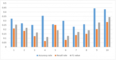
The proposed XGBoost-based prediction model was verified through a prediction experiment on Epinions Trust Network Dataset [17]. Epinions is a website where users can register for free and write reviews on items in various categories (e.g. software, music, television show, hardware, and office appliances). If a review is found useful, the writer will be paid. Table 10 shows the predictions and evaluation results of our model for items in all categories. The prediction cycle was set to one week.
It can be seen that the prediction effect of our model for items in all categories was slightly worse than that for items in a single category. However, the difference is so small as to be negligible. This means our model enjoys fairly good generalization ability on items of all categories.
Figure 2 displays the prediction effects of our model for items in the top 10 categories. The high accuracy, recall and F1 demonstrate the good prediction ability of our model.
Table 10. Predictions and evaluation results of XGBoost-based model for items in all categories
|
Training cycle |
Test cycle |
Accuracy |
Recall |
F1 |
|
9.10-9.14 |
9.15-9.19 |
0.2712 |
0.2231 |
0.2456 |
|
9.10-9.14 |
9.16-9.20 |
0.2463 |
0.2467 |
0.2462 |
|
9.10-9.14 |
9.17-9.21 |
0.2887 |
0.2136 |
0.2453 |
|
9.10-9.14 |
9.18-9.22 |
0.2139 |
0.2702 |
0.2458 |
|
9.10-9.14 |
9.19-9.23 |
0.3519 |
0.2139 |
0.2766 |
|
9.10-9.14 |
9.20-9.24 |
0.2415 |
0.2309 |
0.2366 |
|
9.10-9.14 |
9.21-9.25 |
0.2218 |
0.2861 |
0.2529 |
This paper mainly puts forward a prediction model for purchase intention of ECP users. Firstly, the key features that affect user purchase intention were extracted through feature engineering and big data analysis. Next, the prediction effects of the LR and XGBoost were compared, and the latter was selected as the basis to establish our model. The effectiveness of the XGBoost-based prediction model was verified through an experiment on a real dataset. Our model can accurately predict the probability for ECP users to purchase a category of items in the next 5 days. The research results shed new light on how to improve the consumer stickiness of ECPs.
[1] Azad, N., Safaei, M., Farahani, M.S. (2014). A study on the effects of different factors influencing on customer loyalty, profitability and word of mouth advertisement for gaining competitive advantage in tourism industry. Management Science Letters, 4(6): 1099-1102. https://doi.org/10.5267/J.MSL.2014.5.023
[2] Zhu, Z.G., Wang, J.W., Wang, X.N., Wan, X.J. (2016). Exploring factors of user’s peer-influence behavior in social media on purchase intention: Evidence from QQ. Computers in Human Behavior, 63: 980-987. https://doi.org/10.1016/j.chb.2016.05.037
[3] Lucero, C. (2008). A relationship model between key problems of international purchasing and the post-purchase behavior of industrial firms. The Journal of Business & Industrial Marketing, 23(5): 332-341. https://doi.org/10.1108/08858620810881601
[4] Fargier, H., Gimenez, P.F., Mengin, J. (2018). Recommendation by Bayesian inference. Application to product configuration. Revue d'Intelligence Artificielle, 32(1): 39-74. https://doi.org/10.3166/RIA.32.39-74
[5] Yuan, Z.M., Huang, C., Sun, X.Y., Li, X.X., Xu, D.R. (2015). A microblog recommendation algorithm based on social tagging and a temporal interest evolution model. Frontiers of Information Technology & Electronic Engineering, 16(7): 532-540.
[6] Nanopoulos, A., Rafailidis, D., Symeonidis, P., Manolopoulos, Y. (2010). MusicBox: Personalized music recommendation based on cubic analysis of social tags. IEEE Transactions on Audio Speech & Language Processing, 18(2): 407-412. https://doi.org/10.1109/TASL.2009.2033973
[7] Salter, J., Antonopoulos, N. (2006). CinemaScreen recommender agent: Combining collaborative and content-based filtering. IEEE Intelligent Systems, 21(1): 35-41. https://doi.org/10.1109/MIS.2006.4
[8] Punj, G. (2011). Effect of consumer beliefs on online purchase behavior: The influence of demographic characteristics and consumption values. Journal of Interactive Marketing, 25(3): 134-144. https://doi.org/10.1016/j.intmar.2011.04.004
[9] Lu, J., Hayes, L.A., Yu, C.S. (2009). Improving MIS education in an online learning environment through course-embedded measurement. International Journal of Innovation and Learning, 6(6): 641-658. http://www.inderscience.com/link.php?id=26649
[10] Ahmad, K., Ayyash, M.M., Al-Qudah, O.M.A. (2018). The effect of culture values on consumer intention to use Arabic e-commerce websites in Jordan: An empirical investigation. International Journal of Business Information Systems, 29(2): 155-182. https://doi.org/10.1504/IJBIS.2018.094691
[11] Sun, G., Bin, S. (2018). A new opinion leaders detecting algorithm in multi-relationship online social networks. Multimedia Tools and Applications, 77(4): 4295-4307. https://doi.org/10.1007/s11042-017-4766-y
[12] Lin, W.M., Zhan, T.S., Yang, C.D. (2003). Distribution system reliability worth analysis with the customer cost model based on RBF neural network. IEEE Transactions on Power Delivery, 18(3): 1015-1021. https://doi.org/10.1109/TPWRD.2003.813865
[13] Martin, H.S., Herrero, A. (2012). Influence of the user's psychological factors on the online purchase intention in rural tourism: Integrating innovativeness to the UTAUT framework. Tourism Management, 33(2): 341-350. https://doi.org/10.1016/j.tourman.2011.04.003
[14] Duarte, K., Monnez, J.M., Albuisson, E. (2018). Sequential linear regression with online standardized data. Plos One, 13(1): e0191186. https://doi.org/10.1371/journal.pone.0191186
[15] Guo, Y.J., Ji, D.H. (2014). Summary extraction of news comments based on weighed textual matrix factorization and information entropy model. Journal of Computer Applications, 34(10): 2859-2864. https://doi.org/10.11772/j.issn.1001-9081.2014.10.2859
[16] Cheng, L.C., Wu, C.C., Chen, C.Y. (2019). Behavior analysis of customer churn for a customer relationship system: An empirical case study. Journal of Global Information Management, 27(1): 111-127. https://doi.org/10.4018/JGIM.2019010106
[17] Awal, G.K., Bharadwaj, K.K. (2019). Leveraging collective intelligence for behavioral prediction in signed social networks through evolutionary approach. Information Systems Frontiers, 21: 417-439. https://doi.org/10.1007/s10796-017-9760-4