Modeling the Relationship Between SPT-N Value and Compression Index (Cc) Using Copula Theory for Thi-Qar Clay Soil

Saja Janam![]() | Ressol R. Shakir*
| Ressol R. Shakir*![]()
© 2025 The authors. This article is published by IIETA and is licensed under the CC BY 4.0 license (http://creativecommons.org/licenses/by/4.0/).
OPEN ACCESS
Accurate estimation of the coefficient of compressibility (Cc) is essential for predicting foundation settlement, yet odometer tests on undisturbed samples are often limited in most site investigations. In contrast, standard penetration test (SPT) data are more widely available. Existing SPT–Cc correlations are extremely limited and often inconsistent across soil types, and previous studies relied mainly on linear regression, which cannot capture nonlinear or asymmetric dependence. This study addresses these gaps by developing a probabilistic framework to model the dependency structure between SPT–N₆₀ and Cc for clay soils in Thi-Qar, southern Iraq, using copula theory. Several copula candidates were evaluated using AIC and BIC criteria, and their performance was compared with the classical Nataf model. In addition, the Bootstrap method was adopted as a robust resampling tool to quantify uncertainty in dependence modeling under limited data conditions. The measured data exhibited a moderate negative dependence (ρ = −0.56, τ = −0.43), confirming that denser soils (higher N₆₀) tend to have lower compressibility. Among the tested models, the Gaussian copula provided the best statistical representation of the joint behavior of N₆₀ and Cc. Results also showed that Pearson’s correlation (ρ) is not invariant under monotonic transformations, whereas the Nataf model behaves similarly to the Gaussian copula when dependence is approximately linear. The proposed framework enhances reliability-based characterization of local soils and reduces reliance on extensive laboratory testing by enabling accurate simulation of soil parameters.
bootstrap method, compressibility index, copula theory, correlation, Nataf, SPT
Understanding geotechnical properties such as the coefficient of compressibility (Cc) is essential to foundation design. The calculation of the consolidation settlement depends on the quality of information available from the site and laboratory tests. The standard penetration test (SPT) is one of the most widely used field tests in Iraq and around the world to determine soil resistance. This is because it is simpler and less expensive compared to laboratory tests like the uniaxial compression test. The SPT test was developed in the United States in 1927 [1]. Because of its antiquity and widespread use, studies have presented numerous experimental equations based on its results to evaluate soil properties, such as the correlation of standard penetration number (SPT-N) with relative density (Dr) of sand, undrained cohesion (cu) with SPT-N for clay soil [2], the consistency index (CI), and SPT-N [3]. In many studies, correlations between SPT-N values and sand friction angle have been proposed; a study [4] provided a critical review of these correlations, and a new correlation was proposed based on data collected from the literature. Correlation between SPT-N and the modulus of elasticity (E) has been performed for granular soils [5]. In addition, several studies have examined the correlations between shear wave velocity and SPT-N [6], reviewing the most important of these relationships.
Similarly, the Cc is a crucial metric for assessing the settlement of foundations in clay soils subjected to stresses. Precise and expensive tests in the lab are usually needed to calculate it. Many researchers have taken numerous approaches worldwide to create empirical correlations for compressibility with easily obtainable index properties like void ratio, liquid limit (LL), plasticity index (PI), and natural moisture content [7]. A helpful study for Nasiriyah soil also correlates the compressibility index with Aterberg limits (LL, plastic limit (PL), and PI) [8].
When resources are limited for many projects, it is important to have equations that can estimate soil properties without complex laboratory tests. Empirical relationships about the compressibility index of soil or SPT parameters are thus essential. The compressibility factor has rarely been estimated directly from field test data such as the SPT test. However, some attempts have been made to estimate Cc from SPT data [9]. The researcher used linear regression analysis to determine the relationship between the SPT and the clay soil Cc. The correlation between the soil compression index and SPT-N value of stiff clay soil was linear, as the compression index decreases with increasing SPT-N value, and an unreliable correlation for soft clay. A contrary conclusion was observed for samples included that were collected from different coastal areas, where higher SPT values were associated with higher Cc values [10].
In the domain of probabilistic modeling of geotechnical variables, there exists a necessity to denote the interdependence between parameters, particularly when these variables are not entirely autonomous. Some traditional methods have been applied to accomplish this purpose, such as the Rosenblatt transform [11] and the Nataf transform [12]. However, both approaches face significant restrictions that constrain their proficiency and adaptability. The Rosenblatt transform, alternatively, demands exact foreknowledge of the joint probability density function (PDF), a task that is often extremely complex or impractical, particularly when addressing incomplete data [11]. The Nataf method assumes only a linear relationship between variables and can only be applied to distributions belonging to the normal distribution family, like the Gaussian distribution [13]. This renders it ineffective when the relationship between variables is nonlinear or asymmetrical, as is regularly the case in natural soil properties.
In contrast, the copula theory is a more advanced and flexible option, as it allows for the detachment of marginal distributions from the dependency structure between variables, permitting the precise representation of intricate statistical relationships. The copula does not necessitate a linear relationship and allows the joint cumulative distribution function (CDF) to be constructed independently of marginal distributions [14]. For this reason, the copula has become a widely used instrument in the fields of risk examination, reliability analysis, and geotechnical engineering, particularly when addressing incomplete data. Numerous studies have used copula theory to generate the joint probability distribution of interrelated geotechnical parameters with limited probability distribution information. Uzielli and Mayne [15] used Copula theory to analyze and represent the dependence of load-displacement model parameters to generate samples that account for parametric uncertainties in model inputs, which were then used in a Monte Carlo Simulation (MCS) to assess the impact of these uncertainties on settlement estimation. Wu and Xin [16] used a bivariate copula to simulate the cement fly ash gravelly (CFG), in pile load-settlement behavior regression curve parameter dependence. When probability information is missing, the copula function creates a joint distribution of rockfill material nonlinear strength coefficients [17]. The vine copula was employed in a previous study [18] to model the dependence structure between consolidation parameters such as initial void ratio, compressive index, and saturated density of soft clayey soil, which contributed to providing a more realistic and reliable analysis of consolidation settlement. The copula theory was used in a previous study [19] to model the dependency between uncertain geotechnical design parameters in reliability-based shallow foundation design.
Although the SPT is a common in situ test employed worldwide, and although the Cc is a primary parameter needed for settlement prediction, the literature reveals several critical limitations that motivate the present study. First, SPT–Cc correlations are very scarce and tend to vary with soil type, with some studies noting a decrease in Cc with increasing SPT-N values, and vice versa in other geological settings. Second, past efforts mainly employed simple linear regression, which is an inappropriate tool for modeling linear or asymmetric dependence, which is often the dominant feature of natural soil behaviour, limiting the generalizability of such correlations. Third, to the best of the authors’ knowledge, no prior research has applied copula theory to model the SPT–Cc relationship, whether in Iraq or internationally for regionally representative clay soils, leaving a methodological gap in probabilistic geotechnical modeling. Fourth, in Thi-Qar Governorate, the need for reliable Cc estimation is especially pressing due to the scarcity of undisturbed sampling and the high cost or limited availability of laboratory consolidation tests. Therefore, a probabilistic framework capable of leveraging inexpensive field data such as SPT-N₆₀ to characterize soil compressibility is of practical importance for both routine geotechnical design and reliability-based settlement assessment.
This research aims to develop a copula-based statistical model to describe the relationship between SPT-N60 values and the Cc for clay soils in Thi-Qar Governorate, by integrating real field data with copula dependence structures. The research consists of three parts: the first is collecting the necessary data, then the Copula approach is used to get the dependency, and then simulating the SPT and Cc. The research discussed the marginal distributions of Cc and SPT and the effect of value on the Gaussian copula. Important comparisons with other models are also stated in this research. This research contributes to developing a framework to construct the dependency of Cc and SPT, then includes it in a simulation of the probabilistic state of the two parameters. It is very helpful in examining the reliability analysis and design of shallow foundations and pile foundations.
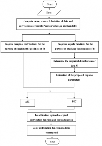
The research methodology is structured into two main components. The first section focuses on the study area, covering the project location and the site geology. The second part deals with the most famous reliability measures, the copula theory, and its most famous types. It also deals with constructing and simulating the joint distribution of SPT-N60 values and the Cc using the copula. Figure 1 shows a flow chart of data simulation using copula functions used in this study.
2.1 Collection of data
The data used in this study were obtained from geotechnical investigation reports of seven different projects located within Thi-Qar Governorate, in southern Iraq, approximately 360 km south of Baghdad, the capital. The studied samples are lean clay collected from seven different projects: two in Nasiriyah, four in Al-Shatra, and one in Al-Nasr, as shown in Figure 2.
At each site, disturbed samples and undisturbed samples were collected using an SPT split spoon and a standard Shelby tube sampler, respectively. One-dimensional consolidation experiments were performed on 17 soil samples, as shown in Table 1. To minimize variability caused by depth differences, all undisturbed samples were taken from a consistent depth range of 4 to 5 meters. The corresponding disturbed samples were collected within ±0.5 meters of the undisturbed sample locations. Therefore, the soil characteristics may be assumed to be the same. The sample size of n = 17 was deemed adequate, given it falls within the range established by previous literature. Wu [20] adopted the sample size of n = 15 in modeling soil shear parameters by copula theory.
Figure 1. Flow chart of data simulation using copula functions

(a)

(b)
Figure 2. Location of the studied region
Table 1. Properties of the soil used in the present study
|
No. |
N60 |
Cc |
|
1 |
8 |
0.2 |
|
2 |
7 |
0.229 |
|
3 |
12 |
0.26 |
|
4 |
13 |
0.18 |
|
5 |
12 |
0.23 |
|
6 |
11 |
0.23 |
|
7 |
4 |
0.34 |
|
8 |
13 |
0.14 |
|
9 |
19 |
0.19 |
|
10 |
5 |
0.229 |
|
11 |
17 |
0.18 |
|
12 |
11 |
0.196 |
|
13 |
13 |
0.19 |
|
14 |
7 |
0.303 |
|
15 |
18 |
0.17 |
|
16 |
7 |
0.19 |
|
17 |
8 |
0.165 |
2.2 Measures of correlation
The dependence between soil parameters describes the relationship between them mathematically or statistically, and means that if one variable changes, the type of change in the other variable will be identified. It shows how each one affects the other and how the other is influenced by this parameter. There are different types of dependence, such as linear, nonlinear, functional, and statistical dependence. Dependence is a critically examined and significant term in probabilistic and statistical analysis, particularly in reliability studies. Stochastic dependency significantly influences not only the development of a joint PDF, but also the assessment of failure probability [13]. Including the dependency between the parameters of soil leads to an accurate analysis and design. Ignoring the dependency may make the design unsafe or conservative, and both shall be avoided.
The joint behavior of the Cc and SPT increases the understanding that will enhance the settlement estimation of the foundation. This will reduce the redundancy in testing to quantify this parameter.
2.2.1 Pearson coefficient (ρ)
Pearson’s ρ correlation coefficient measures the linear dependence between two random variables [21]. It is the most widely used measure of dependency due to its simplicity and close association with the multivariate Gaussian PDF and is expressed as follows:
$\rho=\frac{\operatorname{Cov}\left(X_1, X_2\right)}{\sqrt{\operatorname{var}\left(X_1\right)} \sqrt{\operatorname{var}\left(X_2\right)}}$ (1)
where, ρ $\in$ [-1;+1]. When the value is -1 or +1, this indicates a perfectly linear correlation between the two random variables and no linear relationship when the value equals 0; this does not mean that these two variables are independent, but rather that there is another type of relationship between them [22]. Pearson's correlation coefficient can be expressed in accordance with the notion of covariance:
$\rho=\int_{-\infty}^{+\infty} \int_{-\infty}^{+\infty}\left[\frac{x_1-\mu_1}{\sigma_1}\right]\left[\frac{x_2-\mu_2}{\sigma_2}\right] f\left(x_1, x_2\right) d x_1 d x_2$ (2)
where, μ1 and μ2 represent the means of each of the variables X1 and X2, respectively, σ1 and σ2 are the standard deviations of X1 and X2, and $f\left(x_1, x_2\right)$ is the bivariate distribution function (PDF) of X1 and X2, which is given by:
$f\left(x_1, x_2\right)=D\left(F_1\left(x_1\right), F_2\left(x_2\right) ; \theta\right) f_1\left(x_1\right) f_2\left(x_2\right)$ (3)
By inserting Eq. (3) into Eq. (2), we obtain the relationship between rho Pearson (ρ) and the copula parameter (θ):
$\begin{gathered}\rho=\int_{-\infty}^{+\infty} \int_{-\infty}^{+\infty}\left[\frac{x_1-\mu_1}{\sigma_1}\right]\left[\frac{x_2-\mu_2}{\sigma_2}\right] D\left(F_1\left(x_1\right)^{\prime} F_2\left(x_2\right) ; \theta\right) \\ f_1\left(x_1\right) f_2\left(x_2\right) d x_1 d x_2\end{gathered}$ (4)
It is evident from Eq. (4) that Pearson's correlation coefficient is influenced by both marginal distributions and joint distributions of random variables. However, this contrasts with the copula theorem, which is characterized by separating the dependence structure from the marginal distributions. In addition, the Pearson correlation coefficient is only unchanging in strictly linear monotonic transformations. Suppose non-linear transformations are applied, or the random variables do not follow a joint Gaussian distribution. In that case, it will not be an effective measure of reliability and may lead to incorrect results [23].
2.2.2 Kendall’s $\tau$ coefficient
Kendall’s $\tau$ measures the degree of concordance between random variables. Mathematically, Kendall’s $\tau$ is described as the probability of concordance minus the probability of discordance [24].
$\begin{gathered}\tau=P\left[\left(X_1-\widetilde{X_1}\right)\left(X_2-\widetilde{X_2}\right)>0\right] -P\left[\left(X_1-\widetilde{X_2}\right)\left(X_2-\widetilde{X_2}\right)<0\right]\end{gathered}$ (5)
The first part on the right side represents the concordance probability, and the second part represents the discordance probability. Kendall’s $\tau$ is symmetric and takes values within [-1,1]. In contrast to the linear correlation, Kendall's $\tau$ is unaffected by strictly increasing transformations. Furthermore, it is less sensitive to outliers, so these features have made it the most suitable for representing dependence in copulas [25]. Kendall’s $\tau$ can be articulated in relation to a copula function when the copula (C) is entirely continuous [24, 26].
$\tau=4 \int_0^1 \int_0^1 \mathrm{C}\left(u_1, u_2 ; \theta\right) \mathrm{dC}\left(u_1, u_2 ; \theta\right)-1$ (6)
where, $u_i$ is the CDF of $U_i$ and $U_i=F_i\left(X_i\right)$ represents a standard uniform random variable limited within the interval $[0,1]$. It is evident from Eq. (6) that Kendall's $\tau$ is unaffected by the marginal distributions but only by the adopted copula. When the coefficient of correlation ($\tau$) between $X_1$ and $X_2$ is determined, the value of $\theta$ can be found by repeatedly solving the previous integral equation. The empirical form of Kendall's $\tau$ is expressed as follows:
$\tau=\frac{\sum_{i<j} \operatorname{sign}\left[\left(x_{1 i}-x_{1 j}\right)\left(x_{2 i}-x_{2 j}\right)\right]}{0.5 N(N-1)}$ (7)
where, N represents the number of samples, and the sign(.) is calculated from:
$\operatorname{sign}=\left\{\begin{array}{c}-1\left(x_{1 i}-x_{1 j}\right)\left(x_{2 i}-x_{2 j}\right)<0 \text { (discordant) } \\ 1\left(x_{1 i}-x_{1 j}\right)\left(x_{2 i}-x_{2 j}\right) \geq 0 \text { (concordant) } \\ \mathrm{ij}=1,2 \ldots, \mathrm{~N}\end{array}\right.$ (8)
In this expression, the numerator indicates the difference between the count of concordant and discordant pairs.
2.3 Joint distribution of SPT-N60 and Cc parameters based on copulas
2.3.1 Copulas
Copulas are functions that join several marginal CDFs, intending to construct multivariate CDFs where the dimensional marginal distributions are uniformly distributed throughout the interval [0,1] [24]. The concept of copula theory was originally proposed by Sklar [27]; Sklar’s theorem serves as the cornerstone of copula theory, indicating that a continuous multivariate distribution can be expressed by combining its marginal distributions with a copula describing their dependence structure. Sklar's theory states that the joint distribution can be written as a function based on its marginal distributions, and the copula function is written as in Eq. (9):
$F\left(x_1, x_2\right)=\mathrm{C}\left(F_1\left(x_1\right), F_2\left(x_2\right), \cdots, F_n\left(x_n\right)\right)$ (9)
where, C is a copula function, F1(x1), F2(x2) are marginal distributions.
Since this paper focuses on the relationship between only two variables, SPT and Cc, the bivariate copula function will be introduced. Based on Sklar's theorem, the bivariate CDF, F)x1, x2(, of random variables (X1, X2) is given by:
$F\left(x_1, x_2\right)=C\left(F_1\left(x_1\right), F_2\left(x_2\right)\right)=C\left(u_1, u_2 ; \theta\right)$ (10)
By deriving Eq. (10(, the PDF of the copula function, which can be determined as:
$\begin{aligned} f\left(x_1, x_2\right)= & D\left(F_1\left(x_1\right), F_2\left(x_2\right) ; \theta\right) f_1\left(x_1\right) f_2\left(x_2\right)= D\left(u_1, u_2 ; \theta\right) f_1\left(x_1\right) f_2\left(x_2\right)\end{aligned}$ (11)
where, D(u1,u2;θ) denotes the density function of a bivariate copula, defined by:
$D\left(u_1, u_2 ; \theta\right)=\frac{\partial^2 C\left(u_1, u_2 ; \theta\right)}{\partial u_1 \partial u_2}$ (12)
In this expression, θ is a vector of copula parameters that quantify the dependence between the random variables, and u1 = F1 (X1), u2 = F2 (X2) are uniformly distributed on the interval [0,1].
There are various copulas in the scientific literature; each type has its own properties and dependence structure, including tail dependence, symmetry, and a range of correlation coefficients. These copulas are also classified under families, considering how they are constructed and their similar properties, such as elliptic copulas, Archimedean copulas, and Plackett copulas. In addition, other families of copulas have been used in several fields, such as the Farlie-Gumbel-Morgenstern, Marshall-Olkin, or Ali-Mikhail-Haq copulas; however, these families have limited use in geotechnical applications due to the limited range of accreditation levels they can handle [13]. In this paper, the Gaussian, Plackett, and Archimedean Copulas will be briefly discussed. For a more in-depth explanation, refer to these studies [19, 22].
Gaussian copula
A Gaussian copula is classified as an elliptic copula. It is symmetrical, so it cannot capture asymmetric dependency. In addition, the Gaussian copula has no tail function. Generally, in the case of a bivariate Gaussian distribution, the copula function C(u1, u2; θ) and copula density function c(u1, u2; θ) are given [24]:
$C\left(u_1, u_2 ; \theta\right)=\Phi_\theta\left(\Phi^{-1}\left(u_1\right), \Phi^{-1}\left(u_2\right)\right), \theta \in[-1,1]$ (13)
$c\left(u_1, u_2 ; \theta\right)=\frac{1}{\sqrt{1-\theta^2}} \exp \left[-\frac{\xi_1{ }^2 \theta^2-2 \theta \xi_1 \xi_2+\xi_2{ }^2 \theta^2}{2\left(1-\theta^2\right)}\right]$ (14)
where, $\Phi_\theta$ denotes the bivariate standard normal distribution function, and $\Phi^{-1}$ the inverse of the standard normal distribution function, $\xi_1=\Phi^{-1}\left(u_1\right)$ and $\xi_2=\Phi^{-1}\left(u_2\right)$ are standard normal variables. It is worth noting that the standard univariate normal distribution has a dependence structure uniquely determined by the Gaussian connection [28]. Regarding the copula parameter $\theta$, two common ways exist to estimate this parameter. The first method depends on the Pearson linear correlation coefficient ($\rho$), by solving Eq. (4). The second method is to calculate the copula parameter $\theta$ by the Kendall correlation coefficient, and the relationship between the rho Gaussian ($\theta$) and $\tau$ can be given by:
$\theta=\sin \left(\frac{\pi \tau}{2}\right)$ (15)
The Gaussian copula method, using $\tau$ is more accurate than the method when using the Pearson correlation coefficient. This is because Kendall's $\tau$ does not change under incremental transformations, while Pearson's correlation coefficient does not remain unchanged when nonlinear transformations are applied [29].
Plackett copula
Plackett's copula belongs to the Plackett copula family, and it is an example of copula functions that are built using algebraic methods [24]. The Plackett copula is radially symmetric and has no tail dependence. Moreover, it is a comprehensive copula, which makes it useful for modeling dependence. However, extending the Plackett bivariate copula to include more than two variables is complicated, which is one of its weaknesses. In addition, the relationship between the copula parameter $\theta$ and rank coefficients (such as Kendall's $\tau$) cannot be expressed in a simple mathematical formula, which requires resorting to numerical methods, making the analysis more labor-intensive. The CDF and PDF of the Plackett copula with $\theta \in(0, \infty) \backslash\{1\}$ are, respectively:
$C\left(u_1, u_2 ; \theta\right)=\frac{\mathrm{S}-\sqrt{\mathrm{S}^2-4 u_1 u_2 \theta(\theta-1)}}{2(\theta-1)}$ (16)
where, $\mathrm{S}=1+(\theta-1)\left(u_1+u_2\right)$.
$c\left(u_1, u_2 ; \theta\right)=\frac{\theta\left[1+(\theta-1)\left(\mathrm{u}_1+\mathrm{u}_2-2 \mathrm{u}_1 \mathrm{u}_2\right)\right]}{\left\{\left[1+(\theta-1)\left(\mathrm{u}_1+\mathrm{u}_2\right)\right]^2-4 \mathrm{u}_1 \mathrm{u}_2 \theta(\theta-1)\right\}^{(3 / 2)}}$ (17)
The parameter θ of the Plackett copula is obtained by solving Eq. (6), which defines the relationship between $\tau$ and θ as a double integral.
Archimedean copulas
Archimedean copulas are widely used in geotechnical dependence modeling due to their flexibility, simple construction, efficient sampling, and their ability to represent a broad range of dependence structures. Unlike the Gaussian (normal) copula, Archimedean copulas are built using an explicit generator function that defines the dependence pattern. A general bivariate Archimedean copula can be expressed in closed form as:
$\mathrm{C}\left(u_1, u_2 ; \theta\right)=\varphi_\theta^{-1}\left[\varphi_\theta\left(u_1\right)+\varphi_\theta\left(u_2\right)\right]$ (18)
Nelsen [24] specified conditions that the generator function $\varphi_\theta$ must satisfy the Archimedean copula. These conditions include that the generator function $\varphi_\theta$ must be a continuous function, strictly decreasing, and convex from [0,1] to [0, ∞) so that φθ(0) = ∞, φθ(1) = 0. The scientific literature features numerous generator functions, enabling the construction of various Archimedean copulas.
In geotechnical engineering, four copulas are commonly used for dependence modeling, including the Frank, Gumbel, Clayton, and No.16 copulas. The definitions of the generator function $\varphi_\theta$, copula function C, copula density function c, and range of θ for this family of copulas are given in Table 2.
Frank copula [24] can model both positive and negative dependence, making it a versatile choice for applications, as highlighted by Joe [30]. Frank's copula is symmetrical, and therefore, it may not accurately represent asymmetric relationships. Moreover, it does not exhibit tail dependence [24], which allows it to model dependence at the edges to a certain degree. However, dependence at the extreme edges may not be fully represented, as discussed by Ashkar and Aucoin [31]. Clayton's copula and Gumbel's copula model positive dependency and are asymmetric copulas, with Clayton's copula showing greater dependency in the lower tail, i.e., at low values. In comparison, Gumbel's copula shows greater dependency in the upper tail than in the lower tail. On the contrary, the No.16 copula is characterized by its ability to model negative and weak positive dependencies [13]. Copula 16 is asymmetric, showing a dependency in the lower tail at a low negative correlation coefficient, but as the negative correlation increases, the effect of this dependency becomes less, and the No.16 copula approaches radial symmetry [24].
Table 2. Summary of bivariate Archimedean copulas functions and their dependence parameters [14]
|
Type of Copula |
CDF |
|
Generator $\varphi_{\theta(t)}$ |
Range of θ |
|
Frank |
$-\frac{1}{\theta} \ln \left[1+\frac{\left(e^{-\theta u_1}-1\right)\left(e^{-\theta u_2}-1\right)}{e^{-\theta}-1}\right]$ |
$\frac{-\theta\left(\mathrm{e}^{-\theta}-1\right) e^{\mathrm{e}^{-\theta}\left(u_1+u_2\right)}}{\left[\left(e^{-\theta}-1\right)+\left(e^{-\theta u_1}-1\right)\left(e^{-\theta u_2}-1\right)\right]^2}$ |
$-\ln \frac{e^{-\theta t}-1}{e^{-\theta}-1}$ |
$(-\infty, \infty) \backslash\{0\}$ |
|
Clayton |
$\left[u_1^{-\theta}+u_2^{-\theta}-1\right]^{-1 / 2}$ |
$\frac{(1+\theta)\left(u_1 u_2\right)^{-(\theta+1)}}{\left(u_1-\theta+u_2-\theta-1\right)^{\frac{1+2 \theta}{\theta}}}$ |
$\frac{1}{\theta}\left(\mathrm{t}^{-\theta}-\mathrm{t}\right)$ |
$(0, \infty)$ |
|
Gumbel |
$\exp \left[-\left(\left(-\ln u_1\right)^\theta+\left(-\ln u_2\right)^\theta\right)^{1 / \theta}\right]$ |
$\frac{\exp \left(-S^{\frac{1}{\theta}}\right)\left(\ln u_1 \ln u_2\right)^{\theta-1\left(S^{\frac{1}{\theta}}+\theta+1\right)}}{u_1 u_2 S^{2-\frac{1}{\theta}}}$ $S=\left(-\ln u_1\right)^\theta+\left(-\ln u_2\right)^\theta$ |
$(-\ln t)^\theta$ |
$[1, \infty)$ |
|
No.16 |
$\frac{1}{2}\left(s+\sqrt{s^2+4 \theta}\right)$; $S=u_1+u_2-1-\theta\left(\frac{1}{u_1}+\frac{1}{u_2}-1\right)$ |
$\begin{array}{r}\frac{1}{2}\left(1+\frac{\theta}{u_1^2}\right)\left(1+\frac{\theta}{u_2^2}\right) S^{-(1 / 2)}\left\{-S^{-1}\left[u_1+u_2-1\right.\right. \\ \left.\left.-\theta\left(\frac{1}{u_1}+\frac{1}{u_2}-1\right)\right]^2+1\right\} ;\end{array}$ $S=\left[u_1+u_2-1-\theta\left(\frac{1}{u_1}+\frac{1}{u_2}-1\right)\right]^2$ |
$\left(\frac{\theta}{t}+1\right)(1-t)$ |
$[0, \infty)$ |
For Archimedean copulas, the parameter θ is determined based on Kendall’s $\tau$ between the variables X₁ and X₂ by solving Eq. (6), which, in the case of Archimedean copulas such as Frank and No.16 copulas, reduces from a double to a single integral [24].
$\tau=1+4 \int_0^1 \frac{\varphi_\theta(t)}{\varphi_\theta^{\prime}}(d t)$ (19)
Here, φθ(t) refers to the generator function associated with an Archimedean copula, while φ′θ(t) indicates its first derivative with respect to the variable (t).
2.3.2 Selection of the best-fit marginal distributions and copulas
Certainly, selecting appropriate probability distributions and copulas is fundamental for uncertainty modeling and reliability analysis in geotechnical engineering projects. A wide variety of univariate PDFs have been presented in literature, including continuous and discrete distributions [32], commonly used such as normal, uniform, and logarithmic distributions [13]. Early studies, such as Lumb [33], showed that the normal distribution suitably represents soil strength properties, a view supported by subsequent research [34, 35]. However, more recent work argues that soil properties are inherently non-negative, making the lognormal distribution more suitable in some cases due to the truncation at zero [36, 37]. Generally, the appropriate distribution is chosen through goodness-of-fit tests. Here, the Akaike Information Criterion (AIC) and Bayesian Information Criterion (BIC) [38] are utilized to determine the optimal distribution from among four candidate continuous distributions: Truncated Normal, Truncated Gumbel, Lognormal, and Weibull, as shown in Table 2. These ensure that simulated values remain strictly positive, in accordance with recommendations [14].
Generally, identifying suitable marginal distributions with AIC and BIC entails evaluating several candidates using standard fitting methods (e.g., maximum likelihood or method of moments), with the distribution that attains the lowest AIC and BIC considered the best fit. The AIC is given by:
$A I C=-\sum_{i=1}^N \ln f(x i ; p, q)+2 k_1$ (20)
The BIC is defined as:
$B I C=-2 \sum_{i=1}^N \ln f(x i ; p, q)+k_1 \ln N$ (21)
where, $\ln f(x i ; p, q)$ denotes the log-likelihood function, p and q are the distribution parameters, and k1 indicates how many parameters define the distribution. The merits of these two criteria were considered in a previous study [39].
Similarly, selecting an appropriate copula function—used to model the dependency structure between random variables—is equally critical in probabilistic analysis. The characteristics of copulas differ, particularly with respect to symmetry, the extent of tail dependence, and the types of correlation structures they can model. Although AIC and BIC are commonly applied to identify the best-fitting copula [13], these criteria alone do not ensure correct model selection, especially if all candidate copulas poorly represent the data. Therefore, candidate copulas must be chosen carefully based on their statistical properties.
The AIC and BIC criteria are described as follows, respectively:
$A I C=-2 \sum_{i=1}^N \ln D\left(u_{1 i}, u_{2 i} ; \theta\right)+2 k_2$ (22)
$B I C=-2 \sum_{i=1}^N \ln D\left(u_{1 i}, u_{2 i} ; \theta\right)+k_2 \ln N$ (23)
where, ${{D}}\left(u_{2 i}, u_{2 i} ; \theta\right)$ represents the copula density function, and $\mathrm{k}_2$ denotes the number of copula parameters, and $\left(u_{1 i}, u_{2 i}\right)$ represent realizations of standard uniform random variables (the empirical distribution), which define as:
$\left\{\begin{aligned} u_{1 i} & =\frac{\operatorname{rank}\left(x_{1 i}\right)}{N+1} \\ i & =1,2 \ldots . N \\ u_{2 i} & =\frac{\operatorname{rank}\left(x_{2 i}\right)}{N+1}\end{aligned}\right.$ (24)
where, rank(x1i) represents the rank of x1i among the values x1 when arranged in ascending order. This transformation allows the separation of marginal distributions from the dependence structure, enabling the copula to be modeled independently of the original data distributions.
3.1 Marginal distribution of the N60 and Cc
Initially, it is essential to identify the appropriate marginal distributions. Table 3 includes the candidate marginal distributions. The lowest values of BIC and AIC indicate the best probability distribution that simulates the data [40]. As shown in Table 4, based on the lowest AIC and BIC values, the marginal distributions are estimated to be a Weibull distribution for N60 and a TruncGumbel distribution for Cc. The value of AIC for all the probability distributions is approximately similar to each other. It ranges from 100.9926 to about 103.2645. The narrow range of AIC and BIC may refer to the fact that all the probability distributions fit the data well. However, the lowest value, even with slightly different forms, serves as a basis for comparison between them. The BIC for the second parameter (Cc) was very low values, which refer to a very good fit of the data.
Table 3. Probability density functions and domains of distribution parameters for candidate marginal distributions [14]
|
Marginal Distribution |
Density Function f(x; p, q) |
Remarks |
Range of p |
Range of q |
|
TruncNormal |
$\frac{1}{q \sqrt{2 \pi}} \exp \left[-\frac{1}{2}\left(\frac{x-p}{q}\right)^2\right] /\left[1-\Phi\left(-\frac{p}{q}\right)\right]$ |
$\mu=p, \sigma^2=q^2$ |
$(-\infty, \infty)$ |
$(0, \infty)$ |
|
LogNormal |
$\frac{1}{q x \sqrt{2 \pi}} \exp \left[-\frac{1}{2}\left(\frac{\ln x-p}{q}\right)^2\right]$ |
$\mu=\exp \left(p+0.5 q^2\right)$, $\sigma^2=\left[\exp \left(q^2-1\right)\right] \exp \left(2 q+q^2\right)$ |
$(-\infty, \infty)$ |
$(0, \infty)$ |
|
TruncGumbel |
$\frac{q \exp \{-q(x-p)-\exp [-q(x-p)]\}}{\{1-\exp [-\exp (p q)]\}}$ |
$\mu=p+0.5772 / q$, $\sigma^2=\pi^2 /\left(6 q^2\right)$ |
$(-\infty, \infty)$ |
$(0, \infty)$ |
|
Weibull |
$\frac{q}{p}\left(\frac{x}{p}\right)^{q-1} \exp \left[-\left(\frac{x}{p}\right)^q\right]$ |
$\mu=p \Gamma(1+1 / q)$, $\sigma^2=p^2\left[\Gamma(1+2 / q)-\Gamma^2(1+1 / q)\right]$
|
$(0, \infty)$
|
$(0, \infty)$
|
Table 4. Values of AIC and BIC for different marginal distributions of data
|
Parameter |
TruncNormal |
LogNormal |
TruncGumbel |
Weibull |
||||
|
AIC |
BIC |
AIC |
BIC |
AIC |
BIC |
AIC |
BIC |
|
|
N60 |
101.5981 |
103.2645 |
102.0425 |
103.7089 |
101.7746 |
103.4410 |
100.9926 |
102.6591 |
|
Cc |
−50.0954 |
−48.4289 |
−53.0087 |
−51.3423 |
−53.9799 |
−52.3134 |
−47.7764 |
−46.1100 |

Figure 3. Histograms and PDFs of the best-fitting marginal distributions of the measured dataset
The PDFs of the four candidate marginal distributions are plotted together with the histograms of the measured data in Figure 3. It may visually evaluate the fitting of the probability distribution to the data. This strengthens the capability of the probability distribution to simulate the data.
3.2 General correlation between SPT and Cc
Before modeling the correlation between SPT-N60 and Cc, the measured data are transformed from the original space to a uniform space to facilitate understanding of the relationship and to provide an idea of the appropriate copula. Figure 4 contains the scatter plot in the uniform space obtained after applying Eq. (24), where the effect of the bounded distribution is isolated. The scatter plot in Figure 4 shows a negative correlation between SPT-N60 and Cc. The negative correlation is also verified by Pearson's rho and Kendall's $\tau$ coefficients, which are calculated using Eqs. (1) and (7).
The results showed a negative correlation between SPT-N60 and Cc Pearson’s rho coefficients, and Kendall’s $\tau$ are obtained as −0.5591 and −0.4280, respectively. These findings are consistent with the results reported by Alam et al. [9]. This study showed that an increase in SPT-N values is accompanied by a decrease in Cc values.
The reason for this difference is that Pearson's rho measures linear dependence influenced by the actual values of the data; thus, it is more sensitive to contrarian behavior and outlier values. By contrast, Kendall's $\tau$ captures dependence based on ranks, providing an indication of the general monotonic trend, as opposed to strict linearity.

Figure 4. Scatter plots of the measured dataset
Due to the observed negative correlation, the Gaussian, Plackett, Frank, and No.16 copulas are suitable for describing the dependence between SPT60 and Cc. Thereafter, the copula parameters θ associated with the four prospective copulas, utilizing Eqs. (4) or (15) for the Gaussian copula and Eq. (19) for the Archimedean Copulas are listed in Table 5. After obtaining the copula parameters, the AIC and BIC values are computed for each copula by using Eqs. (22) and (23). Table 5 summarizes the calculated results, where the Gaussian copula is the most suitable because it has the smallest AIC and BIC values.
Table 5. Correlation coefficients of data, copula parameters, AIC, and BIC values of fitted copulas
|
ρ |
$\tau$ |
Gaussian [θ, AIC, BIC] |
Plackett [θ, AIC, BIC] |
Frank [θ, AIC, BIC] |
No.16 [θ, AIC, BIC] |
|
−0.5591 |
−0.4280 |
−0.6228, −6.2054, −5.3722 |
0.1306, −4.6227, −3.7895 |
−4.5607, −5.5567, −4.7235 |
0.0215, −3.3708, −2.5376 |
Given that the available dataset for the variable pair N60–Cc consists of only 17 samples, relying solely on the original sample to estimate probabilistic model parameters or to select the appropriate copula may be unreliable. Small samples are highly sensitive to data fluctuations, as highlighted by Tang et al. [41]. Their study demonstrated that sample size is the most influential factor in identifying the correct copula or marginal distribution, more so than the COV or the distributional shape. Small datasets tend to produce large variability in AIC values, increasing the likelihood of selecting an incorrect model, particularly when the sample size is less than 30. The study also showed that a stronger true dependence reduces the amount of data required for reliable model identification.
To address uncertainty due to a small sample size, Tang et al. [41] recommended using the bootstrap resampling method. The bootstrap method is based on the idea of random sampling with replacement from the original dataset. For the N new samples we created from sample n. This may cause some of the values to appear in more than one row, but also some not to appear on any row. Then we compute the respective statistics for each of the resampled datasets, e.g., mean, standard deviation, copula dependence parameter, and AIC values. By repeating this process many times, every metric gets a sampling distribution that quantifies the uncertainty associated with it and allows for more robust evaluation of probabilistic models. Bootstrap sampling and coupling fit evaluation procedures are a methodology that can be generalized to various probabilistic relationships between geotechnical variables when data is limited [13].
Based on the recommendations of Sepulveda-Garcia and Alvarez [13], a total of N = 10,000 bootstrap samples were adopted to evaluate the uncertainty in the dependence parameter of each copula. For every resampled dataset, the dependence parameter is computed using the method of moments based on Kendall’s $\tau$ for each copula type. After completing all iterations, a set of 10,000 estimated values of the dependence parameter is obtained, forming a sampling distribution that characterizes the uncertainty associated with each copula.
Table 6 shows bootstrap results from 10,000 resampled datasets, indicating unambiguous best-fit results for the Gaussian copula relative to other models. It had the lowest mean AIC value (−6.07) and was selected as the best-fitting model in about 75% of all iterations. This further implies its objectivity and reliability to map the dependency between N60 and Cc, regardless of the limited amount of data points used in the proposed model (17 samples). On the other hand, the Frank and No.16 copulas provided fair performance (selection rates of 11.5% and 12%, respectively), indicating that they are capturing some of the dependence structure, but with less stability than the Gaussian copula. Among them, the Plackett copula demonstrated the poorest performance since it was only selected in 1.57% of cases, having the highest values of AIC, which mirrors its reduced capacity to fit the data.
Table 6. Bootstrap AIC statistics and selection frequencies for candidate copulas
|
Copula Model |
Mean AIC |
Std. AIC |
Number of Best Selections |
Selection Probability (%) |
|
Gaussian |
−6.0704 |
7.5667 |
7493 |
74.93 |
|
Plackett |
−3.8529 |
3.8959 |
157 |
1.57 |
|
Frank |
−5.1533 |
4.8474 |
1150 |
11.5 |
|
No.16 |
−2.3162 |
4.6179 |
1200 |
12 |

Figure 5. Bootstrap PDFs of AIC scores for fitted copulas
Figure 5 shows the AIC distributions for four candidate copulas based on the bootstrap analysis. The Gaussian copula has the lowest AIC values, for most of its distribution tilted to the negative zone, thus confirming its clear temporal superiority as a goodness-of-fit over other models. In comparison, the Frank and No.16 copulas have distributions that are more Gaussian-like; however, they lean toward higher AIC values, indicating reasonable but less stable performance. In contrast, the AIC values for the Plackett copula are consistently lower and more tightly concentrated, indicating a more limited capacity of the Plackett copula to accommodate the dependence between N60 and Cc.
3.3 Generation of data based on a copula
Figure 6 compares the scatter plots of 1000 simulated samples from 17 measured samples using a Gaussian copula with the appropriate marginal distributions. It is worth noting that these simulations were performed using the algorithms presented by Li et al. [23].

Figure 6. Scatter diagrams showing both measured and simulated data using a fitted copula with regression analysis
The scatterplot shows a clear negative, monotonic relationship between N60 and Cc. Linear regression on the measured data yields R2 ≈ 0.31, whereas the copula-based simulated samples reproduce a very similar slope and intercept Cc = −0.007 N60 + 0.288 with a slightly higher explanatory power R2 ≈ 0.36. Since R2 only evaluates how well a straight line fits the data, it can under- or over-state dependence when the true relationship is only partially linear—An effect also reflected by the gap between Pearson’s ρ and Kendall’s $\tau$. Most of the data points are clustered in the mid-range of N60 (8–15) and Cc (0.20–0.30); this clustering increases the scatter around the regression line and explains the relatively low coefficient of determination (R2). Nevertheless, the Gaussian copula was able to successfully reproduce this mid-range concentration, confirming its suitability for capturing the dependence structure between the measured data.
3.4 Comparison of copula shapes with the optimal Gaussian copula
The probability density curves of the proposed copulas were plotted and compared to the optimal copula (Gaussian) with the same margins (Weibull distribution for Cc and Truncgumbel for N60) with $\tau$ = −0.4280, as shown in Figure 7. The results indicate that the Plackett and the Frank fit the Gaussian very closely in the middle of the data, while copula No.16 shows a clear departure from the other copulas, with noticeable variation at the upper and lower ends of the relationship, reflecting its nonlinear nature and asymmetric end dependence when the negative correlation is not strong. This suggests that cupula 16 highlights nonlinear dependence effects that the Gaussian cupula cannot accurately represent.

Figure 7. Iso-density contours for copula models (Gaussian, Plackett, Frank, No.16)
3.5 Effect of t value on the Gaussin copula
Figure 8 demonstrates the variation in the dependence structure of the Gaussian copula for different values of Kendall’s $\tau$, ranging from strong positive to strong negative correlation. Each surface represents the bivariate PDF of the copula in the uniform domain (u1, u2) given the observed data.
The upper row shows when $\tau$ is positive ($\tau$ = 0.90, 0.428, and 0.016) and the corresponding Gaussian ρ = 0.988, 0.623 and 0.025, respectively. When $\tau$ increases, the joint PDF is more peaked along the main diagonal (u₁ ≈ u₂), with the implication of strong positive dependency: Large (or small) values of the one variable tend to occur at the same time that large (or small) values of the other variable occur. As $\tau$ tends to zero, the surface becomes flatter, which suggests a near independence between the two uniform variables; conversely, in the bottom row, where the correlation is negative.
3.6 Nataf versus Gaussian and No.16 copulas
For the purpose of comparison between the Nataf distribution and both the Gaussian copula and Copula No.16, 1,000 samples were simulated based on the dependence structure inferred from the measured data and the best-fitting marginal distributions, as shown in Figure 9. Modeling results indicate that the Nataf transformation exhibits behavior very similar to that of the Gaussian copula when the dependence between the variables is linear or quasi-linear.
When comparing the Nataf transform with copula No.16, which exhibits asymmetry when the negative correlation is weak, the difference becomes clear, while Nataf maintains a symmetric elliptic dependence, copula No.16 exhibits an asymmetric tail behavior, and highlights the nonlinearity between the two variables. Therefore, the Nataf transform is equivalent to the Gaussian copula when the relationship is approximately linear, but it loses accuracy when modeling nonlinear or tail-dependent variables.
The comparison shows that the Nataf transformation cannot describe other nonlinear or tail-dependent behavior between soil parameters since it inherently imposes a symmetric, Gaussian-type dependence structure. On the other hand, copula models like those based on Gaussian and No.16 have a parametric shape of dependence, but this can be learned from data. For the current N60-Cc dataset, it is nearly monotonic and symmetric, so Nataf and the Gaussian copula behave similarly. However, in datasets where soils exhibit stronger nonlinearities or asymmetric tail dependence, the Nataf model may misrepresent the joint variability, whereas copula-based approaches provide a more reliable characterization of the underlying dependence.

Figure 8. 3D surface plot of bivariate density for the Gaussian copula with different values of $\tau$

Figure 9. Simulation of measured data from Nataf distribution, Gaussian, and No.16 copulas
Table 7. Comparison of simulation outcomes related to different dependence models
|
Dependence Model |
$\tau$ (measured) N60-Cc |
ρ (measured) N60-Cc |
$\tau$ (simulated) U1-U2 |
ρ (simulated) U1-U2 |
$\tau$ (simulated) X1-X2 |
ρ (simulated) X1-X2 |
|
Nataf |
−0.4280 |
−0.5590 |
−0.3935 |
−0.5628 |
−0.3935 |
−0.5545 |
|
Gaussian |
−0.4315 |
−0.6078 |
−0.4315 |
−0.6047 |
||
|
No.16 |
−0.4413 |
−0.6250 |
−0.4413 |
−0.6266 |
Both the Pearson correlation coefficient (ρ) and the Kendall correlation coefficient ($\tau$) were calculated for the simulated correlated samples in the uniform (U) space to assess the dependency structure in the copula space. These coefficients were then recalculated in the physical space of variables (X) defined by marginal distributions. The results are summarized in Table 7, which also includes the correlation coefficients measured from the data (N60, Cc).
It is noted that the Kendall coefficient ($\tau$) values between X1 and X2 remained almost constant compared to those calculated between UI and U2 for all the reliability models studied. This is attributed to the stability of the Kendall coefficient against the monotonic transformations used to move from the uniform distribution space U to the physical space X. In contrast, the ρ shows significant variation between the two spaces due to the nonlinear nature of the inverse cumulative distribution transformations used to generate the values of X. In comparison, the Nataf model produced correlation values close to the Gaussian correlation, demonstrating similar linear dependence.
In general, these results validate that $\tau$ is invariant under monotonic transformation, but ρ is influenced by the shape of the marginal distributions. The Nataf model also exhibits similar behavior to the Gaussian copula in representing linear dependence, but differs from copula (16) when describing nonlinear relationships, pointing to the significance of model choice in this case concerning some types of geotechnical data in the non-Gaussian case.
This study demonstrated that copula theory provides a reliable framework for modeling the dependence between SPT–N60 and the compression index Cc in the clay soils of Thi-Qar, where laboratory consolidation data are often unavailable. The Gaussian copula was identified as the most appropriate dependence model, offering a stable representation of the observed negative association and enabling realistic generation of synthetic (N60, Cc) pairs for probabilistic settlement assessment.
The practical significance of the model lies in its ability to provide credible compressibility estimates directly from field test data, thereby supporting reliability-based design and reducing the reliance on extensive laboratory testing. Nevertheless, the approach is sensitive to the limited sample size. Future research should therefore focus on expanding the database, evaluating additional copula families for more complex soil behaviors, and integrating the dependence model into full reliability analyses for settlement prediction.
The authors gratefully acknowledge the support provided by University of Thi-Qar for facilitating data collection required for this study.
[1] Bowles, J.E., Guo, Y. (1996). Foundation Analysis and Design. New York: McGraw-Hill.
[2] Terzaghi, K., Peck, R. (1967). Soil Mechanics in Engineering Practice. New York: John Wiley.
[3] Peck, R.B., Hanson, W.E., Thornburn, T.H. (1974). Foundation Engineering. Wiley.
[4] Duque, J., Acosta, C., Canales, F.A., Cárdenas, J. (2025). On the lookout for a general relationship between the friction angle of sandy soils and SPT. Indian Geotechnical Journal, 1-8. https://doi.org/10.1007/s40098-025-01201-x
[5] Wagh, J.D., Bambole, A.N. (2024). Improved correlation of soil modulus with SPT N values. Open Engineering, 14(1): 20240046. https://doi.org/10.1515/eng-2024-0046
[6] Abbas, H.A., Al-Jeznawi, D., Al-Janabi, M.A.Q., Bernardo, L.F.A., Jacinto, M.A.S.C. (2024). Exploring shear wave velocity—NSPT correlations for geotechnical site characterization: A review. CivilEng, 5(1): 119-135. https://doi.org/10.3390/civileng5010006
[7] Huang, F., Fu, B., Qin, H., Du, Y., Zhu, L., Zhuo, L. (2024). Correlations between physical properties and compression index of fine-grained soils based on a large dataset. IOP Conference Series: Earth and Environmental Science, 1330(1): 012007. https://doi.org/10.1088/1755-1315/1330/1/012007
[8] Mandhour, E.A. (2020). Prediction of compression index of the soil of Al-Nasiriya City using simple linear regression model. Geotechnical and Geological Engineering, 38(5): 4969-4980. https://doi.org/10.1007/s10706-020-01339-w
[9] Alam, M.J., Shaha, N.R., Shohug, M.K. (2015). Relationship between standard penetration resistance and strength-compressibility parameters of clay. Journal of Civil Engineering (IEB), 43(2): 115-131.
[10] Urmi, Z.A., Ansary, M.A. (2019). Interpretation of compressibility characteristics for coastal soil of Bangladesh. In Proceedings on International Conference on Disaster Risk Management, Dhaka, Bangladesh, pp. 129-134.
[11] Cui, X.Y., Hu, X.B., Zeng, Y. (2017). A Copula-based perturbation stochastic method for fiber-reinforced composite structures with correlations. Computer Methods in Applied Mechanics and Engineering, 322: 351-372. https://doi.org/10.1016/j.cma.2017.05.001
[12] Lebrun, R., Dutfoy, A. (2009). An innovating analysis of the Nataf transformation from the copula viewpoint. Probabilistic Engineering Mechanics, 24(3): 312-320. https://doi.org/10.1016/j.probengmech.2008.08.001
[13] Sepulveda-Garcia, J.J., Alvarez, D.A. (2022). On the use of copulas in geotechnical engineering: A tutorial and state-of-the-art-review. Archives of Computational Methods in Engineering, 29(7): 4683-4733. https://doi.org/10.1007/s11831-022-09760-5
[14] Phoon, K.K., Ching, J. (Eds.). (2015). Risk and Reliability in Geotechnical Engineering. CRC Press.
[15] Uzielli, M., Mayne, P.W. (2012). Load-displacement uncertainty of vertically loaded shallow footings on sands and effects on probabilistic settlement estimation. Georisk: Assessment and Management of Risk for Engineered Systems and Geohazards, 6(1): 50-69. https://doi.org/10.1080/17499518.2011.626333
[16] Wu, X.Z., Xin, J.X. (2019). Probabilistic analysis of site-specific load-displacement behaviour of cement-fly ash-gravel piles. Soils and Foundations, 59(5): 1613-1630. https://doi.org/10.1016/j.sandf.2019.07.003
[17] Song, L.F., Xu, B., Kong, X.J., Zou, D.G., Yu, X., Pang, R. (2021). Reliability analysis of 3D rockfill dam slope stability based on the copula function. International Journal of Geomechanics, 21(3): 04021001. https://doi.org/10.1061/(ASCE)GM.1943-5622.0001932
[18] Senapati, S., Dey, A.K., Dutta, S. (2025). Reliability analysis for consolidation settlement of a shallow footing based on copula model. International Journal of Civil Engineering, 23: 815-830. https://doi.org/10.1007/s40999-025-01075-3
[19] Liu, X.F., Tang, X.S., Li, D.Q. (2019). Impact of copula selection on reliability-based design of shallow foundations. In the 7th International Symposium on Geotechnical Safety and Risk (ISGSR 2019), Taipei, Taiwan, China. https://doi.org/10.3850/978-981-11-2725-0-IS14-9-cd
[20] Wu, X.Z. (2015). Modelling dependence structures of soil shear strength data with bivariate copulas and applications to geotechnical reliability analysis. Soils and Foundations, 55(5): 1243-1258. https://doi.org/10.1016/j.sandf.2015.09.023
[21] Mari, D.D., Kotz, S. (2001). Correlation and Dependence. World Scientific. https://doi.org/10.1142/p226
[22] Ang, A.H.S., Tang, W.H. (2007). Probability Concepts in Engineering Planning and Design: Emphasis on Application to Civil and Environmental Engineering. Wiley.
[23] Li, D.Q., Tang, X.S., Phoon, K.K., Chen, Y.F., Zhou, C.B. (2013). Bivariate simulation using copula and its application to probabilistic pile settlement analysis. International Journal for Numerical and Analytical Methods in Geomechanics, 37(6): 597-617. https://doi.org/10.1002/nag.1112
[24] Nelsen, R.B. (2006). An Introduction to Copulas. New York, NY: Springer.
[25] McNeil, A.J., Frey, R., Embrechts, P. (2015). Quantitative Risk Management: Concepts, Techniques and Tools-Revised Edition. Princeton University Press.
[26] Schweizer, B., Wolff, E.F. (1981). On nonparametric measures of dependence for random variables. The Annals of Statistics, 9(4): 879-885. https://doi.org/10.1214/aos/1176345528
[27] Sklar, M. (1959). Fonctions de répartition à n dimensions et leurs marges [in French]. Annales de l'ISUP, 8(3): 229-231. https://hal.science/hal-04094463v1.
[28] Lebrun, R., Dutfoy, A. (2009). A generalization of the Nataf transformation to distributions with elliptical copula. Probabilistic Engineering Mechanics, 24(2): 172-178. https://doi.org/10.1016/j.probengmech.2008.05.001
[29] Li, D., Tang, X., Zhou, C., Phoon, K.K. (2012). Uncertainty analysis of correlated non-normal geotechnical parameters using Gaussian copula. Science China Technological Sciences, 55(11): 3081-3089. https://doi.org/10.1007/s11431-012-4937-z
[30] Joe, H. (1997). Multivariate Models and Multivariate Dependence Concepts. CRC Press. https://doi.org/10.1201/9780367803896
[31] Ashkar, F., Aucoin, F. (2011). A broader look at bivariate distributions applicable in hydrology. Journal of Hydrology, 405(3-4): 451-461. https://doi.org/10.1016/j.jhydrol.2011.05.043
[32] Kottegoda, N.T., Rosso, R. (2008). Applied Statistics for Civil and Environmental Engineers. Blackwell Publishing.
[33] Lumb, P. (1970). Safety factors and the probability distribution of soil strength. Canadian Geotechnical Journal, 7(3): 225-242. https://doi.org/10.1139/t70-032
[34] Liang, R.Y., Nusier, B.O., Malkawi, A.H. (1999). A reliability based approach for evaluating the slope stability of embankment dams. Engineering Geology, 54(3-4): 271-285. https://doi.org/10.1016/S0013-7952(99)00017-4
[35] Baecher, G.B., Christian, J.T. (2005). Reliability and Statistics in Geotechnical Engineering. John Wiley & Sons.
[36] Brejda, J.J., Moorman, T.B., Smith, J.L., Karlen, D.L., Allan, D.L., Dao, T.H. (2000). Distribution and variability of surface soil properties at a regional scale. Soil Science Society of America Journal, 64(3): 974-982. https://doi.org/10.2136/sssaj2000.643974x
[37] Fenton, G.A., Griffiths, D.V. (2003). Bearing-capacity prediction of spatially random c-φ soils. Canadian Geotechnical Journal, 40(1): 54-65. https://doi.org/10.1139/t02-086
[38] Schwarz, G. (1978). Estimating the dimension of a model. The Annals of Statistics, 6(2): 461-464. https://doi.org/10.1214/aos/1176344136
[39] Burnham, K.P., Anderson, D.R. (2004). Multimodel inference: Understanding AIC and BIC in model selection. Sociological Methods & Research, 33(2): 261-304. https://doi.org/10.1177/0049124104268644
[40] Shakir, R.R. (2019). Selecting the probability distribution of cone tip resistance using moment ratio diagram for soil in Nasiriyah. Geotechnical and Geological Engineering, 37(3): 1703-1728. https://doi.org/10.1007/s10706-018-0716-3
[41] Tang, X.S., Li, D.Q., Cao, Z.J., Phoon, K.K. (2017). Impact of sample size on geotechnical probabilistic model identification. Computers and Geotechnics, 87: 229-240. https://doi.org/10.1016/j.compgeo.2017.02.019