Ajaykumar Kakde*![]() | Manisha Dale
| Manisha Dale![]()
© 2025 The authors. This article is published by IIETA and is licensed under the CC BY 4.0 license (http://creativecommons.org/licenses/by/4.0/).
OPEN ACCESS
This study proposes a hybrid deep learning (DL) framework that integrates sentiment-derived features from financial news with technical stock indicators to enhance stock price forecasting accuracy. Sentiment metrics, specifically polarity and subjectivity scores, were extracted from the Economic Times 2024 dataset using VADER and TextBlob, and combined with technical parameters within a modified Stacked Long Short-Term Memory (SLSTM) model capable of capturing sequential market dependencies. The proposed framework was tested on four major NIFTY 50 companies representing the IT, banking, pharmaceutical, and metal sectors. Experimental evaluation showed notable gains in prediction accuracy, with Mean Absolute Error (MAE) values ranging from 1.67 to 20.31, Root Mean Squared Error (RMSE) from 2.08 to 26.49, and R² consistently exceeding 0.96. Comparative results showed that models incorporating polarity and subjectivity variables outperformed those utilizing only compound sentiment, highlighting the importance of detailed linguistic cues. Overall, the study found that using multi-source features considerably improves prediction stability and accuracy. The proposed architecture provides a scalable, domain-flexible solution for sentiment-driven financial forecasting, facilitating the development of intelligent stock market (SM) decision-support systems.
SM, SP, SLSTM, TDS, TA, SA, financial news analysis, DL
The stock market (SM), noted for its intricacy and volatility, has historically captivated researchers and investors alike who are in pursuit of effective methodologies to forecast price fluctuations and render informed choices. Precise prediction of SM trends is imperative for optimizing returns and alleviating risks.
Conventional methodologies have predominantly depended on technical analysis, which scrutinizes historical price data, trends and trading volumes to project future market behaviour. Nevertheless, these approaches frequently neglect the significant impact of financial news, social media posts and public sentiments, which may lead to quick changes in the market.
Over recent years, sentiment analysis (SA) [1, 2] has surfaced as a formidable instrument for distilling signals pertinent to the market obtained from text-based sources such as market-related news reports, online social platforms and expert analysis. By quantifying investor sentiment, this methodology offers critical context that augments technical indicators.
Compared to using either technique alone, combining SA and TA has demonstrated a great deal of potential in improving predictive accuracy. The SM is a crucial element of the global economy, working as a platform for capital management and an indicator of economic health. Accurate SM prediction is very important for traders, investors, financial experts and analysts as financial markets grow more complex.
Though widely used, traditional stock market analysis techniques like TA and fundamental analysis (FA) frequently miss the subtle patterns and fluctuations found in financial data. Traditional methods used only historical data of SM for future predictions.
In the modern era, deep learning (DL) has emerged as a transformative approach in the field of SM prediction, offering fresh chances to improve predictive accuracy and dependability.
Stock price (SP) forecasting has been attempted through various approaches, mainly categorized into following three core methodologies as shown below in Figure 1.
Figure 1. Methods for SM analysis
FA assesses the true intrinsic value of a stock by conducting an analysis of the financial health of company from financial statements and profit performance, growth potential, industry position and broader economic conditions.
To find market trends, patterns and price movements that might point to future price changes, TA looks at historical price data, trading volume and market indicators. These trends are frequently analysed using tools like Moving Averages, Bollinger Bands and Momentum Indicators.
SA, a new field in natural language processing (NLP), examines textual data from news headlines, financial blogs and online forums to determine the general sentiment or opinion of investors. It captures the psychology of the market, which frequently affects price direction without reference to fundamental value. Both FA and TA have drawbacks, such as their incapacity to identify noise in data and to adjust to the quickly changing market conditions.
Stock market forecasting has been transformed by the advent of DL algorithms. Large-scale datasets can contain intricate, non-linear patterns that can be captured by DL models, particularly those that use neural networks. They are particularly beneficial for forecasting time series problems, which forecasts future values based on historical data, because of this capability.
With the evolution of artificial intelligence [2], machine learning (ML) and DL techniques have become popular in SM prediction because of their capacity to record complex temporal dependencies and represent nonlinear interactions. In time-series forecasting, algorithms like Support Vector Machines (SVM), Random Forests (RF), and more recently, DL models like Long Short-Term Memory (LSTM) and Convolutional Neural Networks (CNN) have produced promising results.
Because of the erratic and unpredictable behaviour of financial markets, predicting SP trends is inherently difficult. However, these predictions are now more accurate than ever before because of advancements in big data analytics, artificial intelligence and processing power. Achieving high forecasting accuracy is crucial because it directly aids in the development of profitable investment portfolios. While DL techniques have shown promising results in identifying trends in large datasets, no model has consistently generated accurate forecasts of future stock prices.
The following are the primary contributions of this research:
Comprehensive experiments were conducted involving multiple runs and hyperparameter optimization. A benchmark configuration was established—specifying ideal neuron numbers per layer, epochs and batch size—to guide future advancements in predictive model design.
2.1 SVM and DL models
Ren et al. [1] combined an SVM and SA to forecast the direction of the SSE 50 Index's trend and a forecasting accuracy of 89.93% was achieved. Shen et al. [2] proposed a DL model in which feature engineering and multiple techniques were combined for short-term stock price predictions and traditional methods were outperformed. Arif et al. [3] evaluated the integration of TA with ML algorithms and Neural Networks were found to yield the best results. Muhammad et al. [4] proposed a DL technique for stock trend prediction and accuracy of 94.9% was attained with interpretability enhanced through XAI techniques such as SHAP and LIME. Akhtar et al. [5] concluded that the RF algorithm achieved the greatest accuracy across the studied ML methods. Vrtagic and Mourched [6] combined information about gold futures, Bitcoin and the NASDAQ-100 for gold price prediction which achieves high accuracy (R2 = 0.98) using ML model.
2.2 LSTM and BiLSTM based models
Mehta et al. [7] demonstrated that social media sentiment, when incorporated using LSTM, improved prediction accuracy to approximately 92.45%. Khonde et al. [8] developed a web application through which financial news sentiment was analyzed, resulting in 86% accuracy in headline categorization and 83% accuracy in stock performance forecasting. Mu et al. [9] suggested the MS-SSA-LSTM model, in which investor’s sentiment and historical trading data were integrated, and an average R² improvement of 10.74% over standard LSTM was achieved by optimizing hyperparameters using the Sparrow Search Algorithm. Albahli et al. [10] introduced a DL framework combining Deep Contextualized Word Representation (DCWR) and Hierarchical Attention Networks (HANet) and a prediction accuracy of 92.5% was attained. Gite et al. [11] presented a model in which LSTM was combined with SA of financial news data, resulting in a prediction accuracy of 74.76% while Explainable AI (XAI) techniques were utilized. Thormann et al. [12] utilized LSTM networks with Twitter SA to enhance predictions for Apple stock prices. Elminaam et al. [13] presented a Bidirectional LSTM model with a global pooling mechanism, where RMSE values of 0.413, 0.704 and 0.478 were achieved thus demonstrating efficiency for real-time applications. Ko et al. [14] utilized LSTM neural networks combined with SA from financial news sources and forum discussions to forecast SP and an average RMSE improvement of 12.05% was achieved. It was concluded that SA significantly enhances SP prediction accuracy. Sidek et al. [15] examined the influence of news sentiment on Bursa Malaysia's SM using LSTM and prediction accuracy was significantly improved with RMSE values recorded below one. Rochman et al. [16] suggested that for classification purpose LSTM gives better accuracy than Naïve Bayes, SVM and Backpropagation methods.
Chandola et al. [17] presented a hybrid model integrating Word2Vec and LSTM and an accuracy of 65.4% in predicting stock direction was achieved, emphasizing the role of SA.
Safari and Badamchizadeh [18] introduced DeepInvesting, a multimodal DL model using a Sequence-Oriented, Long-Term Dependent BiLSTM architecture for stock price prediction, where exceptional forecasting performance on Amazon Corp. (AMZN) data with minimal MAPE and high R² values was demonstrated.
2.3 CNN and hybrid approaches
Kasture and Shirsath [19] proposed a hybrid RNN-LSTM model where SA was integrated, resulting in a MAE of 0.036 and a RMSE of 0.046. Song and Choi [20] introduced hybrid models, including CNN-LSTM and GRU-CNN, which outperformed standard techniques in 48.1% and 81.5% of cases for one-time-step and multi-time-step forecasting respectively.
Agrawal et al. [21] developed an Evolutionary Deep Learning Model (EDLM) and prediction accuracies of 63.59% for HDFC, 56.25% for Yes Bank and 57.95% for SBI were recorded.
Correia et al. [22] explored various deep learning architectures, with CNNs achieving 73% training accuracy and 69% test accuracy. Raza et al. [23] employed LSTM and GRU models integrating historical stock prices and macroeconomic indicators and improved prediction accuracy was demonstrated.
Nabipour et al. [24] explored various ML techniques including decision trees and LSTM and LSTM was found to outperform conventional models. Yang et al. [25] proposed a hybrid CNN-LSTM model and superior prediction accuracy through a three-dimensional input tensor was achieved. Bhandari et al. [26] implemented LSTM networks for predicting S&P 500 indices, with significantly fewer prediction errors than conventional techniques being reported.
Lawi et al. [27] investigated LSTM and GRU models and significant prediction accuracy improvements with eight proposed architectures were achieved. Jing et al. [28] developed a fusion model in which CNN was used for classifying sentiment and SP prediction using LSTM and performance improvements across six industries were validated. Zhang et al. [29] developed a CNN-BiLSTM-Attention model DL algorithms which were employed to improve stock index projections' accuracy.
2.4 Sentiment and technical data fusion studies
Ardisurya and Rizkinia [30] implemented a Diffusion Variational Autoencoder (D-VAE) model, where a MSE of 2753.204 and an R² of 0.94489 were achieved, highlighting the significant role of SA in enhancing SP prediction.
Liu et al. [31] proposed SA-TrellisNet, which integrated sentiment analysis from economic news articles with stock market data using a Trellis Network and competitive results across seven major indices were achieved. Ge [32] developed a hybrid model, in which Multivariate Empirical Mode Decomposition and Aquila Optimizer were combined with LSTM to predict S&P 500 and CSI 300 prices.
Pham et al. [33] introduced a new investor sentiment index designed to isolate irrational behavioral biases and improved SM performance prediction was shown. Chaudhari and Mahajan [34] presented a deep reinforcement learning approach combining SA with technical indicators and high prediction accuracy was achieved.
Gumus and Sakar [35] found that models that included sentiment data surpassed those that depended solely on historical prices. Most of research used RNN, CNN, LSTM, BiLSTM and CNN-LSTM model for prediction by combining sentiment score and technical data.
In contrast to previous studies that focused exclusively on compound sentiment analysis, this research implements a fusion of polarity and subjectivity features within an enhanced stacked LSTM architecture, leading to greater model interpretability and improved generalization performance across diverse market sectors.
The structure of the paper is as follows: An introduction is given in Section I. Section II presents a summary of related literature. The approach and models are explained in Section III. The updated stacked LSTM model that produces sentiment-driven predictions is described in Section IV. The experimental results and related commentary are presented in Section V. Finally, A brief summary of the study is given in Section VI, along with potential avenues for future investigation.
The framework used for extracting and analyzing sentiment data from news articles in the Economic Times for selected companies of NIFTY 50, from January 1, 2024, to December 31, 2024. The companies under consideration include Infosys, Sun Pharma, Tata Steel and HDFC Bank.
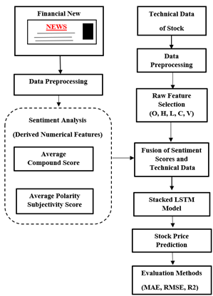
Figure 2 illustrates a hybrid framework for SP prediction using a fusion of SA and TDS given to an SLSTM model.
Figure 2. Flow diagram illustrating stock price prediction process
Financial news was pre-processed and analyzed for SA to derive numerical features such as the average compound score and average polarity-subjectivity score. Simultaneously, technical stock data was pre-processed and key features such as open, high, low, close, and volume (O, H, L, C, V) were selected. These sentiment and technical features were fused and fed into an SLSTM model for training and prediction. The proposed model’s forecasting performance was assessed using MAE, RMSE and R² for robust evaluation.
3.1 Data acquisition
The study incorporates two independent data sets. The primary dataset consists of raw stock data from the National Stock Exchange (NSE) for selected stocks. The stock data included parameters such as date, time, opening price, closing price, highest price, lowest price and trading volume, recorded at specific intervals.
The second dataset comprised news articles obtained from the Economic Times.
3.1.1 Financial data
Data collected from NSE India for the time period of 1st January 2024 to 31st December 2024 [36]. Table 1 shows sample data set for TDS.
Table 1. Sample dataset for TDS
|
Date |
Series |
Open |
High |
Low |
P. Close |
Close |
Volume |
|
31-Dec-24 |
EQ |
136.87 |
138.68 |
136.56 |
136.88 |
138.05 |
20080291 |
|
30-Dec-24 |
EQ |
138.91 |
139.25 |
136.09 |
138.91 |
136.88 |
32555723 |
|
27-Dec-24 |
EQ |
140.7 |
141.75 |
138.61 |
140.36 |
138.91 |
19562177 |
|
26-Dec-24 |
EQ |
140.95 |
141.15 |
139.51 |
140.38 |
140.36 |
23939932 |
|
24-Dec-24 |
EQ |
141.2 |
141.5 |
139.25 |
141.71 |
140.38 |
25882917 |
3.1.2 Sentiment data
Sentiment data for Infosys, Sun Pharma, Tata Steel and HDFC Bank were collected from the Economic Times news during the same time frame [37].
The Economic Times provides more reliable and domain-specific finance news data compared to Google News, specifically in relation to financial analysis.
3.2 Data preprocessing and feature extraction
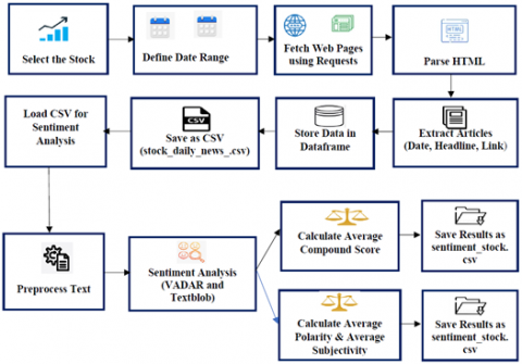
The proposed framework presents an automated workflow for conducting SA on finance related news of specific stocks using web scraping and NLP techniques as shown below in Figure 3.
Figure 3. Block diagram for web scraping and SA score
The process started by selecting a target stock and defining a specific date range to retrieve the relevant news data.
The sentiment analysis process was carried out in Python 3.10, utilizing the Natural Language Toolkit (NLTK v3.9) and TextBlob v0.17.1 libraries. The VADER Sentiment Intensity Analyzer operated with its standard lexicon thresholds (positive ≥ 0.05, negative ≤ –0.05 and neutral = 0). Polarity and subjectivity measures were obtained through TextBlob’s built-in functions, employing default tokenization settings without additional filters. All experimental procedures were executed in Jupyter Notebook version 6.5.4, with model implementation carried out using TensorFlow 2.14 and Keras 3.0. A fixed random seed value of 42 was applied across all tests to maintain consistency and reproducibility of results.
The HTML data was subsequently processed using libraries such as BeautifulSoup to retrieve key components, such as publication dates and news headlines.
This information was structured and stored in a Pandas DataFrame and subsequently saved as a CSV file for further analysis. Table 2 shows the sample dataset for SA.
Table 2. Sample dataset for SA
|
Date |
Headline |
|
01-01-2024 |
bharti airtel services to acquire 97.1 stake in beetel teletech |
|
01-01-2024 |
vodafone idea shares hit fresh 52-week high jump up to 37 in two sessions |
|
01-01-2024 |
sjvn gets govt approval to form jvs for 8778 mw hydro renewable projects |
|
01-01-2024 |
lic gets rs 806 crore gst demand notice |
|
01-01-2024 |
eicher motors gets rs 130 cr tax demand notices company to challenge |
|
01-01-2024 |
ultratech cement slapped with two gst demand orders totalling rs 72 lakh |
In the next phase, the saved CSV file containing stock-related news was loaded for SA. Before analysis, the text was pre-processed by removing noise such as punctuation and stop words, converting the text to lowercase and standardizing the format and then SA was carried out by different methods.
In SA the term compound was used to denote the compound score, a normalized value that reflected the aggregate sentiment of a text. This score ranged from -1 (indicating the most negative sentiment) to +1 (indicating the most positive sentiment). It was calculated based on a blend of positive, negative and neutral sentiment scores generated by tools such as VADER.
Let Cn be the compound score for the nth sentence or text. N be the total number of sentiment-scored sentences.
Average Compound Score $=\frac{1}{n} \sum_{n=1}^N C_n$ (1)
Table 3 shows the average compound score of SA. In SA, two essential metrics, the polarity score and the subjectivity score, were often used to figure out how people felt about a piece of writing.
Table 3. Average compound score
|
Date |
Average Compound Score |
|
01-01-2024 |
0.049486 |
|
02-01-2024 |
0.029134 |
|
03-01-2024 |
0.047019 |
|
04-01-2024 |
0.057271 |
|
05-01-2024 |
0.077117 |
|
06-01-2024 |
0.100317 |
|
07-01-2024 |
0.254651 |
|
08-01-2024 |
0.128624 |
|
09-01-2024 |
0.141211 |
|
10-01-2024 |
0.10751 |
|
11-01-2024 |
0.04186 |
|
12-01-2024 |
0.082584 |
|
13-01-2024 |
0.045652 |
|
14-01-2024 |
0.050501 |
The polarity score, which typically ranged from -1 to 1, indicated which sentiment was most prevalent in the text. Scores near -1 denoted extremely pessimistic sentiment where as scores near +1 denoted intense optimism and scores near 0 denoted neutrality.
Tools such as TextBlob were used to evaluate a sentence's or document's emotional tone. On the other hand, the subjectivity score, which ranges from 0 to 1, shows how much the content is influenced by personal opinions rather than objective facts. A score close to 0 indicates an objective or factual tone, whereas a score close to 1 suggests that the text expresses biases, personal opinions or feelings.
Let Pn represent the polarity score of the nᵗʰ sentence or text, Sn denote its subjectivity score and N indicate the total number of sentences for which sentiment scores have been computed.
Average Polarity Score $=\frac{1}{n} \sum_{n=1}^N P_n$ (2)
Average Subjectivity Score $=\frac{1}{n} \sum_{n=1}^N S_n$ (3)
Table 4 shows the calculated average polarity and average subjectivity score of SA.
Table 4. Average polarity and average subjectivity score
|
Date |
Average Polarity Score |
Average Subjectivity Score |
|
01-01-2024 |
0.075676543 |
0.259543 |
|
02-01-2024 |
0.048220131 |
0.232371 |
|
03-01-2024 |
0.066767988 |
0.232908 |
|
04-01-2024 |
0.037966 |
0.232346 |
|
05-01-2024 |
0.074815228 |
0.239358 |
|
06-01-2024 |
0.106262626 |
0.26182 |
|
07-01-2024 |
0.245929614 |
0.284868 |
|
08-01-2024 |
0.100485089 |
0.232868 |
|
09-01-2024 |
0.153023436 |
0.255381 |
|
10-01-2024 |
0.075741209 |
0.212553 |
|
11-01-2024 |
0.064629314 |
0.198292 |
|
12-01-2024 |
0.057744176 |
0.225406 |
|
13-01-2024 |
0.05164661 |
0.233889 |
|
14-01-2024 |
0.056708691 |
0.196836 |
In the final step, the average compound score as well as average polarity and average subjectivity score for the news articles of a specific stock for the specific time frame were calculated by combining all sentiment values.
The calculated sentiment scores were saved in separate CSV files (sentiment_stock.csv, for instance), which can subsequently be used for financial prediction or quantitative analysis tasks.
This flexible and scalable framework enabled a data-driven interpretation of market sentiment, helping with tasks like algorithmic trading, investor behavior analysis and risk evaluation by turning unstructured news content into organized and useful insights.
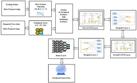
4.1 Modified stacked LSTM architecture
LSTM networks [38] address vanishing gradient problem by using memory cells and gates to retain information over longer periods, making them effective for capturing SM trends.
Figure 4 presents a modified SLSTM model for predicting next-day stock opening prices, integrating technical data with sentiment scores.
Figure 4. Modified stacked LSTM architecture
4.2 Mathematical presentation of modified stacked LSTM model
A Sequential Keras (SK) model was constructed, comprising: two LSTM layers, each with 100 units. The first LSTM layer returned sequences, while the second processed the sequence output.
Input Sequence – at each time step t, input sequence is
$X=\left\{ {{X}_{1}},{{X}_{2}},{{X}_{3}},\ldots ,\ldots ,{{X}_{Ts}} \right\}$ (4)
where, T = seq_len, n = number of features.
First LSTM Layer – Equations
$\text{Forget }\!\!~\!\!\text{ gate}:\text{ }\!\!~\!\!\text{ }{{\text{f}}_{\text{ts}}}^{1}=\text{ }\!\!\sigma\!\!\text{ }{{\text{W}}_{\text{f}}}^{1}.\left[ {{\text{h}}_{\text{ts}-1}}^{1},\text{ }\!\!~\!\!\text{ }{{\text{x}}_{\text{ts}}} \right]+{{\text{b}}_{\text{ts}}}^{1}$ (5)
$\text{Input }\!\!~\!\!\text{ Gate}:\text{ }\!\!~\!\!\text{ }{{\text{i}}_{\text{ts}}}^{1}=\text{ }\!\!\sigma\!\!\text{ }{{\text{W}}_{\text{i}}}^{1}.\left[ {{\text{h}}_{\text{ts}-1}}^{1},\text{ }\!\!~\!\!\text{ }{{\text{x}}_{\text{ts}}} \right]+{{\text{b}}_{\text{is}}}^{1}$ (6)
$\text{Cell } \text{ State}:\text{ }\!\!~\!\!\text{ }\widetilde{{\text{C}}_{\text{ts}}}^{1}=\text{tanh}{{\text{W}}_{\text{c}}}^{1}.\left[ {{\text{h}}_{\text{ts}-1}}^{1},\text{ }\!\!~\!\!\text{ }{{\text{x}}_{\text{ts}}} \right]+{{\text{b}}_{\text{cs}}}^{1}$ (7)
$\text{CS }\!\!~\!\!\text{ Update}:{{\text{C}}_{\text{ts}}}^{1}={{\text{f}}_{\text{ts}}}^{1}\text{*}{{\text{C}}_{\text{ts}-1}}^{1}+{{\text{i}}_{\text{ts}}}^{1}\text{*}{{\widetilde{{{\text{C}}_{\text{ts}}}}}^{1}}$ (8)
$\text{Output }\!\!~\!\!\text{ gate}:\text{ }\!\!~\!\!\text{ }{{\text{O}}_{\text{ts}}}^{1}=\text{ }\!\!\sigma\!\!\text{ }{{\text{W}}_{\text{o}}}^{1}.\left[ {{\text{h}}_{\text{ts}-1}}^{1},\text{ }\!\!~\!\!\text{ }{{\text{x}}_{\text{ts}}} \right]+{{\text{b}}_{\text{os}}}^{1}$ (9)
$\text{Hidden }\!\!~\!\!\text{ State}:\text{ }\!\!~\!\!\text{ }{{\text{h}}_{\text{ts}}}^{1}={{\text{o}}_{\text{ts}}}^{1}\odot \text{tanh }\!\!~\!\!\text{ }{{\text{C}}_{\text{ts}}}^{1}$ (10)
The first LSTM layer computed hidden states and output the full sequence$\{{{\text{h}}_{1}}^{\left( 1 \right)},{{\text{h}}_{2}}^{\left( 1 \right)},..{{\text{h}}_{\text{Ts}}}^{\left( 1 \right)}\}$.
Dropout layer 1 (0.2 rate) was applied after each LSTM layer to mitigate overfitting.
${\widetilde{\mathrm{h}_{\mathrm{ts}}}}^1=$ Dropout$\left(\mathrm{h}_{\mathrm{ts}}{ }^1\right.$, Rate $\left.=0.2\right)$ (11)
The second LSTM layer processed this sequence and output only the final hidden state as a single vector. Another dropout layer was applied.
$\mathrm{h}_{\mathrm{ts}}{ }^2=\operatorname{LSTM}^2\left(\left\{\mathrm{~h}_{\mathrm{ts}}{ }^1, \mathrm{~h}_{1 \mathrm{~s}}{ }^1, \ldots, \mathrm{~h}_{\mathrm{Ts}}{ }^1\right\}\right)$ (12)
Dropout layer 2 (0.2 rate) was applied after each LSTM layer to mitigate overfitting.
$\tilde{\mathrm{H}}_{\mathrm{ts}}{ }^2=$ Dropout$\left(\mathrm{h}_{\mathrm{Ts}}{ }^2\right.$, Rate $\left.=0.2\right)$ (13)
Finally, a dense layer performed a linear transformation to produce the final prediction for the regression task.
$\hat{y}=W_d \cdot\hbar^2+b_d$ (14)
Here, $\hat{y}$ is the predicted output, Wd is weight matric and bd is bias term added for linear transformation.
Here, σ denotes the sigmoid activation function, while $\odot ~$indicates the Hadamard (element-wise) operation. The variables h and C represent the hidden and cell states of the LSTM, respectively. W and b correspond to the weight matrices and bias components and t signifies the time step. All parameters are expressed in normalized form, with input features scaled between 0 and 1 to maintain numerical stability and improve training efficiency.
4.3 SLSTM model—integration of TDS with compound score
Technical features were merged with the average compound score of SA of news data. (OPEN, HIGH, LOW, CLOSE, VOLUME, average_compound_score) were selected and the OPEN price was designated as the prediction target. After merging stock and sentiment data, the final input vector was:
${{X}_{t}}=\left[ {{O}_{t,}}{{H}_{t}},{{L}_{t}},{{C}_{t}},{{V}_{t}},Cs \right]$ (15)
Here, $Cs$ denotes average compound score.
All numerical features were scaled to a 0 to 1 range using MinMaxScaler to optimize neural network training.
These values were fed to the SLSTM model. This time series data was transformed into sequences of seven past trading days using a custom create_sequence() function, where each sequence was used to forecast the next day's opening price. The data was segmented into two portions, with 80% employed for training and 20% reserved for model performance assessment.
4.4 SLSTM model—integration of TDS with polarity and subjectivity score
Technical features were fused with the average polarity and average subjectivity score from SA of news data.
(OPEN, HIGH, LOW, CLOSE, VOLUME, average_polarity, average subjectivity) were selected, and the OPEN price was designated as the prediction target.
After merging stock and sentiment data, the final input vector was:
${{X}_{t}}=\left[ {{O}_{t,}}{{H}_{t}},{{L}_{t}},{{C}_{t}},{{V}_{t}},{{P}_{t,}}{{S}_{t}} \right]$ (16)
Here, ${{P}_{t,}}{{S}_{t}}$ denotes average polarity and subjectivity score.
All numerical features were scaled to a 0-1 range using MinMaxScaler to optimize neural network training. These values were fed into the SLSTM model, this time series data was transformed into sequences of seven past trading days using a custom create_sequence() function, where each sequence was used to predict the subsequent day's opening price.
For evaluation purposes, 80% of the dataset was designated for training and 20% for testing.
4.5 Training and evaluation
The model was optimized using the Adam optimizer with MSE as the loss function. It was trained for 100 epochs (EP) with a batch size (BS) of 16.
A grid search approach was used to optimize the hyperparameters, where different combinations of neuron counts {50, 100}, batch sizes {16, 32}, and epochs {50, 100} were systematically tested. The setup with 100 neurons, 100 epochs, and a batch size of 16 produced the lowest validation RMSE (2.08 for Tata Steel) and was therefore chosen as the optimal configuration. To prevent overfitting, early stopping and dropout regularization (set at 0.2) were also applied during training.
The precision and reliability of SM forecasting models were evaluated using various statistical and performance metrics. The test dataset was evaluated using MAE, RMSE and the coefficient of determination (R²).
A hybrid model was developed for SP prediction by combining SA and TDS within a Stacked LSTM framework. Financial news was processed and analyzed for sentiment to generate quantitative features, including the average compound score and average polarity-subjectivity score. The following evaluation methods were utilized in SM prediction:
5.1 MAE
It quantifies the average magnitude of absolute differences between predicted outputs and actual observations, without considering the direction of the errors.
MAE is calculated as:
$MAE=\frac{1}{n}\underset{i=1}{\overset{n}{\mathop \sum }}\,\left| {{y}_{is}}-\widehat{{{y}_{is}}} \right|$ (17)
where, n denotes the number of observations.
${{y}_{\text{is}}}$ denotes the variable's actual value at the ith observation, and $\hat{\mathrm{y}}_{\mathrm{is}}$ denotes the expected value of a variable at the ith observation.
5.2 MSE
It represents the average of the squared differences between the observed and predicted values.
MSE is calculated as:
$M S E=\frac{1}{n} \sum_{i=0}^n\left(y_{i s}-\widehat{y_{l s}}\right)^2$ (18)
5.3 RMSE
It is an often-used metric in SM forecasting because of its ability to quantify prediction accuracy, sensitivity to errors, interpretability, comparability and suitability for optimization.
RMSE is calculated as:
$\text{RMSE}=\sqrt{\text{MSE}}$ (19)
5.4 R2
R2 is an indicator of the accuracy of predictions in relation to actual data.
R2 is calculated as:
${{R}^{2}}=1-\frac{\sum {{\left( {{y}_{is}}-{{{\hat{y}}}_{is}} \right)}^{2}}}{\sum {{\left( {{y}_{is}}-{{{\bar{y}}}_{is}} \right)}^{2}}}$ (20)
Table 5 shows the performance of SLSTM model when integrating compound score with technical data. The best setup for the SLSTM model, which combines stock technical data and compound sentiment scores, is 100 neurons, 100 EP and a batch size of 16, which produces the highest prediction accuracy for all stocks.
Table 5. Performance of stacked LSTM model integrating compound score with technical data
|
Evaluation Methods |
NIFTY Sectoral Indices |
Stock Name |
Stacked LSTM Model - Compound Score with Technical Data |
|||||||
|
Neurons - 50 |
Neurons - 100 |
|||||||||
|
Ep-50 |
Ep-100 |
Ep-50 |
Ep-100 |
|||||||
|
BS-16 |
BS-32 |
BS-16 |
BS-32 |
BS-16 |
BS-32 |
BS-16 |
BS-32 |
|||
|
MAE |
Nifty IT |
INFOSYS |
27.65 |
30.9 |
22.08 |
26.99 |
25.12 |
32.33 |
18.34 |
22.56 |
|
Nifty Metals |
TATA STEEL |
2.62 |
2.865 |
2.12 |
4.26 |
2.47 |
2.74 |
1.72 |
2.29 |
|
|
Nifty Bank |
HDFC BANK |
26.49 |
27.66 |
19.81 |
28.67 |
20.04 |
31.42 |
17.64 |
27.99 |
|
|
Nifty Pharma |
SUNPHARMA |
24.98 |
21.82 |
20.2 |
27.38 |
21.83 |
22.98 |
20.31 |
29.53 |
|
|
RMSE |
Nifty IT |
INFOSYS |
35.2 |
39.03 |
28.3 |
33.62 |
32.49 |
41.17 |
23.85 |
29.03 |
|
Nifty Metals |
TATA STEEL |
3.32 |
3.67 |
2.66 |
5.24 |
3.01 |
3.48 |
2.16 |
2.92 |
|
|
Nifty Bank |
HDFC BANK |
37.37 |
40.91 |
28.4 |
39.57 |
31.8 |
41.7 |
26.49 |
35.94 |
|
|
Nifty Pharma |
SUNPHARMA |
30.26 |
28.3 |
25.14 |
32.8 |
27.09 |
28.85 |
25.1 |
35.31 |
|
|
R2 |
Nifty IT |
INFOSYS |
0.96 |
0.95 |
0.97 |
0.96 |
0.96 |
0.94 |
0.96 |
0.97 |
|
Nifty Metals |
TATA STEEL |
0.93 |
0.92 |
0.95 |
0.84 |
0.94 |
0.93 |
0.97 |
0.92 |
|
|
Nifty Bank |
HDFC BANK |
0.92 |
0.9 |
0.95 |
0.91 |
0.94 |
0.9 |
0.96 |
0.92 |
|
|
Nifty Pharma |
SUNPHARMA |
0.97 |
0.97 |
0.98 |
0.96 |
0.97 |
0.97 |
0.97 |
0.9 |
|
With the lowest MAE values—TATA STEEL (1.72), HDFC BANK (17.64) and INFOSYS (18.34)—this configuration clearly improves forecasting accuracy. INFOSYS (23.85), TATA STEEL (2.16) and HDFC BANK (26.49) all have lower RMSE values, which suggests improved model stability and fewer prediction errors. The R-Squared (R²) values, which reach 0.97 for TATA STEEL and SUNPHARMA and 0.96 for INFOSYS, confirm a robust correlation between expected and actual stock performance.
According to the MAE comparison, prediction errors were greatly reduced by combining polarity and subjectivity features, by as much as 16.3% for Sun Pharma and 2.9% for Tata Steel.
Overall, using more neurons and epochs, training the model with a smaller batch size, and combining sentiment scores with technical indicators greatly improves the model's capacity to comprehend market trend. This results in predictions of stock prices that are more accurate and consistent.
Table 6 shows the performance of SLSTM model when integrating average polarity and subjectivity score with technical data. Using 100 neurons, a batch size of 16, and 100 epochs yields the highest accuracy and consistency in predictions for all examined stocks, according to the evaluation of the SLSTM model, which integrates technical stock indicators with objectivity–subjectivity sentiment measures.
Table 6. Performance of stacked LSTM model integrating polarity–subjectivity score with technical data
|
Evaluation Methods |
NIFTY Sectoral Indices |
Stock Name |
Stacked LSTM Model - Polarity Subjectivity Score with Technical Data |
|||||||
|
Neurons - 50 |
Neurons - 100 |
|||||||||
|
Ep-50 |
Ep-100 |
Ep-50 |
Ep-100 |
|||||||
|
BS-16 |
BS-32 |
BS-16 |
BS-32 |
BS-16 |
BS-32 |
BS-16 |
BS-32 |
|||
|
MAE |
Nifty IT |
INFOSYS |
26.9 |
29.07 |
21.99 |
26.92 |
30.39 |
29.2 |
17.04 |
24.28 |
|
Nifty Metals |
TATA STEEL |
3.48 |
3.08 |
2.24 |
2.56 |
2.34 |
2.85 |
1.67 |
2.32 |
|
|
Nifty Bank |
HDFC BANK |
30.2 |
30.63 |
21.24 |
22.57 |
35.39 |
25.19 |
17.25 |
19.87 |
|
|
Nifty Pharma |
SUNPHARMA |
21.07 |
23.57 |
21.04 |
24.66 |
20.94 |
26.96 |
17 |
22.13 |
|
|
RMSE |
Nifty IT |
INFOSYS |
34.56 |
36.97 |
28.68 |
35.66 |
1547.9 |
38.11 |
23.07 |
32.442 |
|
Nifty Metals |
TATA STEEL |
4.2 |
3.82 |
2.8 |
3.27 |
2.96 |
3.61 |
2.08 |
3 |
|
|
Nifty Bank |
HDFC BANK |
40.35 |
44.72 |
30.69 |
37.02 |
42.27 |
38.43 |
24.18 |
29.9 |
|
|
Nifty Pharma |
SUNPHARMA |
26.93 |
28.91 |
26.53 |
30.53 |
26.51 |
32.3 |
21.99 |
27.63 |
|
|
R2 |
Nifty IT |
INFOSYS |
0.96 |
0.95 |
0.97 |
0.96 |
0.95 |
0.95 |
0.98 |
0.968 |
|
Nifty Metals |
TATA STEEL |
0.89 |
0.91 |
0.95 |
0.93 |
0.95 |
0.92 |
0.97 |
0.94 |
|
|
Nifty Bank |
HDFC BANK |
0.9 |
0.88 |
0.94 |
0.92 |
0.9 |
0.91 |
0.97 |
0.95 |
|
|
Nifty Pharma |
SUNPHARMA |
0.97 |
0.97 |
0.97 |
0.97 |
0.97 |
0.96 |
0.98 |
0.97 |
|
With the lowest MAE values, this configuration clearly improves prediction accuracy, especially for TATA STEEL (1.67), INFOSYS (17.04) and HDFC BANK (17.25). Additionally, there are smaller differences between the expected and actual prices, as indicated by the lower RMSE values for TATA STEEL (2.08) and INFOSYS (23.07). Strong agreement between model predictions and actual market data is demonstrated by the R2 values, which are still high at 0.98 for INFOSYS and SUNPHARMA and above 0.95 for the majority of other stocks.
An average drop of roughly 10% is seen in the RMSE comparison, suggesting increased prediction accuracy. Overall, the outcomes demonstrate that the model works better when more neurons and epochs are used with a smaller batch size. The hybrid SLSTM model produces accurate and dependable stock price predictions by combining sentiment-based features with technical stock data to better understand market behavior.
Table 7 demonstrates that the SLSTM model outperformed the compound sentiment score when trained with polarity–subjectivity sentiment scores.
Table 7. Comparative study of compound score and polarity-subjectivity scores in a stacked LSTM model
|
Evaluation Methods |
Stock Name |
SLSTM Model _100 Neurons_100 EP_16 Batch Size |
|
|
Compound Score |
Polarity and Subjectivity Score |
||
|
BS - 16 |
BS - 16 |
||
|
MAE |
INFOSYS |
18.34 |
17.04 |
|
TATA STEEL |
1.72 |
1.67 |
|
|
HDFC BANK |
17.64 |
17.25 |
|
|
SUNPHARMA |
20.31 |
17 |
|
|
RMSE |
INFOSYS |
23.85 |
23.07 |
|
TATA STEEL |
2.16 |
2.08 |
|
|
HDFC BANK |
26.49 |
24.18 |
|
|
SUNPHARMA |
25.1 |
21.99 |
|
|
R2 |
INFOSYS |
0.96 |
0.98 |
|
TATA STEEL |
0.97 |
0.97 |
|
|
HDFC BANK |
0.96 |
0.97 |
|
|
SUNPHARMA |
0.97 |
0.98 |
|
The confidence intervals of 95% for R2 were computed using bootstrapping (n = 1000) in order to evaluate reliability. With skewness less than 0.2 and kurtosis less than 3, the error distribution plots displayed nearly normal behavior, indicating steady predictions free from systematic bias.
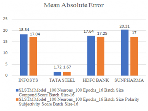
Using polarity–subjectivity sentiment scores consistently resulted in lower error rates, as shown in Figure 5. As an illustration of improved forecasting accuracy, the MAE for TATA STEEL fell from 1.72 to 1.67 and for SUNPHARMA it fell from 20.31 to 17.00.
Figure 5. Performance comparison of MAE for SLSTM model for compound and polarity subjectivity score
Lower RMSE values, which indicate smaller prediction errors, were obtained when polarity–subjectivity sentiment scores were used, as shown in Figure 6. For example, SUN PHARMA's RMSE dropped from 25.10 to 21.99, and TATA STEEL's RMSE decreased from 2.16 (with compound scores) to 2.08, indicating less prediction variability.
Figure 6. Performance comparison of RMSE for SLSTM model for compound and polarity subjectivity score
The R2 coefficients derived from polarity–subjectivity scores were more strongly correlated with actual stock prices, as seen in Figure 7. An average improvement of about 0.02 and better predictive alignment were demonstrated by INFOSYS, which obtained an R2 of 0.98 as opposed to 0.96 with compound scores.
Figure 7. Performance comparison of R2 for SLSTM model for compound and polarity subjectivity score
5.5 Key contribution of the proposed methodology
Finally, the integration of technical indicators and polarity-subjectivity sentiment metrics improves the predictive accuracy of the Stacked LSTM model, reduces forecasting errors and aligns actual stock price movements more closely than the use of compound sentiment scores alone. Table 8 shows the comparison of the suggested methodology's performance with cutting-edge techniques
Table 8. Performance comparison of proposed methodology with state-of-the-art methods
|
References |
Methodology |
Results |
Drawback |
Relevance to Present Work |
|
[20] |
Hybrid CNN-LSTM and GRU-CNN |
48.1% (1-step), 81.5% (multi-step) improvement |
Computationally intensive |
Demonstrates deep learning utility |
|
[30] |
a Diffusion Variational Autoencoder (D-VAE) |
MSE of 2753.204 and R² of 0.94489 |
Complex architecture, higher training cost |
Proves sentiment boosts prediction accuracy |
|
[19] |
Hybrid RNN-LSTM with sentiment integration |
MAE = 0.036, RMSE = 0.046 |
Requires high-quality sentiment data |
Validates sentiment integration in prediction |
|
[32] |
MEMD + Aquila Optimizer + LSTM |
RMSE = 27.12 (S&P500), 56.66 (CSI 300) |
Complexity in hybrid design |
Highlights robustness in volatile conditions. |
The results demonstrated the model’s reliable predictive performance and its ability to generalize across different stocks. Furthermore, the marginally higher R2 values obtained with polarity–subjectivity scores imply that this sentiment feature combination better captures market behavior, enhancing the SLSTM framework's prediction accuracy.
Although only four NIFTY 50 companies were examined in this study, they offer a snapshot of a range of market dynamics and represent a number of industries, including banking, pharmaceuticals, metals and information technology. The dataset used in this study was relatively small. Future studies could be improved by looking at a larger sample of NIFTY 50 stocks or extending the timeframe over several years in order to more accurately evaluate the model's generalization and stability across different sectors.
The positive outcomes from comparing compound sentiment scores with polarity-subjectivity scores indicate several future research directions. One promising strategy to enhance stock price forecasting and more accurately capture investor sentiment in financial news is to combine different sentiment scoring techniques, such as compound scores with deep contextual embeddings from models like BERT.
Extending the dataset to include full-length news articles, social media posts, financial blogs of analysts, government policies, global impact and in-depth financial reports could yield richer insights. Applying the LSTM framework to a broader set of stocks and industries would also validate its robustness and generalizability. Developing an automated prediction system with visual sentiment tracking and real-time data could be very helpful for traders. Further research into sophisticated deep learning architectures, like GRU and attention-based models, could increase the precision of sentiment-driven financial forecasting.
There are two ways to incorporate advanced contextual embeddings like BERT into the current framework: either concatenating BERT-generated sentence vectors with technical indicators at the embedding level or processing these embeddings through parallel dense layers before combining them at the feature level. With this method, the model would be able to identify deeper semantic relationships and more intricate linguistic patterns in textual data.
The first author carried out all aspects of the research, including conceptualization, data collection, signal processing, model development and manuscript writing, under the guidance of the second author. The second author offered critical feedback, technical supervision and overall direction throughout the study.
|
Ps |
Polarity Score |
|
Ss |
Objectivity Score |
|
Cs |
Compound Score |
|
${{\text{f}}_{\text{ts}}}^{1}$ |
Forget Gate of LSTM first Layer |
|
${{\text{i}}_{\text{ts}}}^{1}$ |
Input Gate of LSTM first Layer |
|
${{\widetilde{{{\text{C}}_{\text{ts}}}}}^{1}}$ |
Cell State of LSTM first Layer |
|
${{\text{C}}_{\text{ts}}}^{1}$ |
Cell State Update of LSTM first Layer |
|
${{\text{O}}_{\text{ts}}}^{1}$ |
Output Gate of LSTM first Layer |
|
${{\text{h}}_{\text{ts}}}^{1}$ |
Hidden State of LSTM first Layer |
[1] Ren, R., Wu, D.D., Liu, T.X. (2019). Forecasting stock market movement direction using sentiment analysis and support vector machine. IEEE Systems Journal, 13(1): 760-770. https://doi.org/10.1109/JSYST.2018.2794462
[2] Shen, J., Shafiq, M.O. (2020). Short-term stock market price trend prediction using a comprehensive deep learning system. Journal of Big Data, 7: 66. https://doi.org/10.1186/s40537-020-00333-6
[3] Arif, E., Suherman, S., Widodo, A.P. (2024). Integration of technical analysis and machine learning to improve stock price prediction accuracy. Mathematical Modelling of Engineering Problems, 11(11): 2929-2943. https://doi.org/10.18280/mmep.111106
[4] Muhammad, D., Ahmed, I., Naveed, K., Bendechache, M. (2024). An explainable deep learning approach for stock market trend prediction. Heliyon, 10(21): e40095. https://doi.org/10.1016/j.heliyon.2024.e40095
[5] Akhtar, M.M., Zamani, A.S., Khan, S., Shatat, A.S.A., Dilshad, S., Samdani, F. (2022). Stock market prediction based on statistical data using machine learning algorithms. Journal of King Saud University - Science, 34(1): 18-27. https://doi.org/10.1016/j.jksus.2022.101940
[6] Vrtagic, S., Mourched, B. (2025). A machine learning approach to gold price prediction using financial indicators. International Journal of Computational Methods and Experimental Measurements, 13(1): 199-210. https://doi.org/10.18280/ijcmem.130120
[7] Mehta, P., Pandya, S., Kotecha, K. (2021). Harvesting social media sentiment analysis to enhance stock market prediction using deep learning. PeerJ Computer Science, 7: e476. https://doi.org/10.7717/peerj-cs.476
[8] Khonde, S.R., Virnodkar, S.S., Nemade, S.B., Dudhedia, M.A., Kanawade, B., Gawande, S.H. (2024). Sentiment analysis and stock data prediction using financial news headlines approach. Revue d'Intelligence Artificielle, 38(3): 999-1008. https://doi.org/10.18280/ria.380325
[9] Mu, G.Y., Gao, N., Wang, Y.H., Dai, L. (2023). A stock price prediction model based on investor sentiment and optimized deep learning. IEEE Access, 11: 51353-51367. https://doi.org/10.1109/ACCESS.2023.3278790
[10] Albahli, S., Awan, A., Nazir, T., Irtaza, A., Alkhalifah, A., Albattah, W. (2022). A deep learning method DCWR with HANet for stock market prediction using news articles. Complex & Intelligent Systems, 8: 2471-2487. https://doi.org/10.1007/s40747-022-00658-0
[11] Gite, S., Khatavkar, H., Kotecha, K., Srivastava, S., Maheshwari, P., Pandey, N. (2021). Explainable stock prices prediction from financial news articles using sentiment analysis. PeerJ Computer Science, 7: e340. https://doi.org/10.7717/peerj-cs.340
[12] Thormann, M.L., Farchmin, J., Weisser, C., Kruse, R.M., Säfken, B., Silbersdorff, A. (2021). Stock price predictions with LSTM neural networks and twitter sentiment. Statistics, Optimization & Information Computing, 9(2): 268-287. https://doi.org/10.19139/soic-2310-5070-1202
[13] Elminaam, D.S.A., El-Tanany, A.M.M., El Fattah, M.A., Salam, M.A. (2024). StockBiLSTM: Utilizing an efficient deep learning approach for forecasting stock market time series data. International Journal of Advanced Computer Science and Applications, 15(4): 442-451. https://doi.org/10.14569/IJACSA.2024.0150446
[14] Ko, C.R., Chang, H.T. (2021). LSTM-based sentiment analysis for stock price forecast. PeerJ Computer Science, 7: e408. https://doi.org/10.7717/peerj-cs.408
[15] Sidek, Z., Ahmad, S.S.S., Teo, N.H.I. (2023). Associating deep learning and the news headlines sentiment for Bursa stock price prediction. Indonesian Journal of Electrical Engineering and Computer Science, 31(2): 1041-1049. https://doi.org/10.11591/ijeecs.v31.i2.pp1041-1049
[16] Rochman, E.M.S., Miswanto, Suprajitno, H., Rachmad, A., Mula’ab, Santosa, I. (2023). Utilizing LSTM and K-NN for anatomical localization of tuberculosis: A solution for incomplete data. Mathematical Modelling of Engineering Problems, 10(4): 1114-1124. https://doi.org/10.18280/mmep.100403
[17] Chandola, D., Mehta, A., Singh, S., Tikkiwal, V.A., Agrawal, H. (2023). Forecasting directional movement of stock prices using deep learning. Annals of Data Science, 10: 1361-1378. https://doi.org/10.1007/s40745-022-00432-6
[18] Safari, A., Badamchizadeh, M.A. (2024). DeepInvesting: Stock market predictions with a sequence-oriented BiLSTM stacked model – A dataset case study of AMZN. Intelligent Systems with Applications, 24: 200439. https://doi.org/10.1016/j.iswa.2024.200439
[19] Kasture, P., Shirsath, K. (2024). Enhancing stock market prediction: A hybrid RNN-LSTM framework with sentiment analysis. Indian Journal of Science and Technology, 17(18): 1880-1888. https://doi.org/10.17485/IJST/v17i18.466
[20] Song, H., Choi, H. (2023). Forecasting stock market indices using the recurrent neural network based hybrid models: CNN LSTM, GRU-CNN, and ensemble models. Applied Sciences, 13(7): 4644. https://doi.org/10.3390/app13074644
[21] Agrawal, M., Shukla, P.K., Nair, R., Nayyar, A., Masud, M. (2022). Stock prediction based on technical indicators using deep learning model. Computers, Materials & Continua, 70(1): 287-302. https://doi.org/10.32604/cmc.2022.014637
[22] Correia, F., Madureira, A.M., Bernardino, J. (2022). Deep neural networks applied to stock market sentiment analysis. Sensors, 22(12): 4409. https://doi.org/10.3390/s22124409
[23] Raza, A., Javed, M., Fayad, A., Khan, A.Y. (2023). Advanced deep learning-based predictive modelling for analyzing trends and performance metrics in stock market. Journal of Accounting and Finance in Emerging Economies, 9(3): 277-294. https://doi.org/10.26710/jafee.v9i3.2739
[24] Nabipour, M., Nayyeri, P., Jabani, H., Mosavi, A., Salwana, E., S, S. (2020). Deep learning for stock market prediction. Entropy, 22(8): 840. https://doi.org/10.3390/e22080840
[25] Yang, C., Zhai, J.J., Tao, G.H. (2020). Deep learning for price movement prediction using convolutional neural network and long short-term memory. Mathematical Problems in Engineering, 2020: 2746845. https://doi.org/10.1155/2020/2746845
[26] Bhandari, H.N., Rimal, B., Pokhrel, N.R., Rimal, R., Dahal, K.R., Khatri, R.K.C. (2022). Predicting stock market index using LSTM. Machine Learning with Applications, 9: 100320. https://doi.org/10.1016/j.mlwa.2022.100320
[27] Lawi, A., Mesra, H., Amir, S. (2022). Implementation of long short-term memory and gated recurrent units on grouped time-series data to predict stock prices accurately. Journal of Big Data, 9: 89. https://doi.org/10.1186/s40537-022-00597-0
[28] Jing, N., Wu, Z., Wang, H.F. (2021). A hybrid model integrating deep learning with investor sentiment analysis for stock price prediction. Expert Systems with Applications, 178: 115019. https://doi.org/10.1016/j.eswa.2021.115019
[29] Zhang, J.L., Ye, L.S., Lai, Y.Z. (2023). Stock price prediction using CNN-BiLSTM-attention model. Mathematics, 11(9): 1985. https://doi.org/10.3390/math11091985
[30] Ardisurya, Rizkinia, M. (2024). Implementation of diffusion variational autoencoder for stock price prediction with the integration of historical and market sentiment data. International Journal of Economics, Business and Entrepreneurship, 2(2): 229-242. https://doi.org/10.62146/ijecbe.v2i2.55
[31] Liu, W.J., Ge, Y.B., Gu, Y.C. (2024). News-driven stock market index prediction based on trellis network and sentiment attention mechanism. Expert Systems with Applications, 250: 123966. https://doi.org/10.1016/j.eswa.2024.123966
[32] Ge, Q. (2025). Enhancing stock market forecasting: A hybrid model for accurate prediction of S&P 500 and CSI 300 future prices. Expert Systems with Applications, 260: 125380. https://doi.org/10.1016/j.eswa.2024.125380
[33] Pham, Q., Pham, H., Pham, T., Tiwari, A.K. (2025). Revisiting the role of investor sentiment in the stock market. International Review of Economics & Finance, 100: 104089. https://doi.org/10.1016/j.iref.2025.104089
[34] Chaudhari, A.Y., Mahajan, S. (2025). Prediction of stock market using sentiment analysis and ensemble learning. MethodsX, 14: 103260. https://doi.org/10.1016/j.mex.2025.103260
[35] Gumus, A., Sakar, C.O. (2021). Stock market prediction in Istanbul Stock Exchange by combining stock price information and sentiment analysis. International Journal of Advanced Engineering and Pure Sciences, 33(1): 18-27. https://doi.org/10.7240/jeps.683952
[36] National Stock Exchange of India. https://www.nseindia.com.
[37] The Economic Times. https://economictimes.indiatimes.com/.
[38] Colah. (2015). Understanding LSTMs Networks. https://colah.github.io/posts/2015-08-Understanding-LSTMs/.