R. Vikram![]() | V. Maheswari*
| V. Maheswari*![]()
© 2025 The authors. This article is published by IIETA and is licensed under the CC BY 4.0 license (http://creativecommons.org/licenses/by/4.0/).
OPEN ACCESS
In this article, a graph-theoretical framework is employed to analyze the structural characteristics of key interconnection networks - butterfly, benes, and mesh-derived networks (MDNs): MDN1 and MDN2, through the application of bond-additive molecular descriptors, particularly the Adriatic indices. The aim is to quantitatively assess the efficiency and strength of these networks using tools from chemical graph theory. Each network is represented as a graph, and various forms of Adriatic indices are computed analytically, incorporating different edge-weighting schemes. These indices effectively characterize topological features such as connectivity, regularity, redundancy, and fault tolerance. The findings indicate that butterfly and benes networks exhibit high regularity with limited redundancy, whereas MDNs demonstrate enhanced fault tolerance and scalability. This consistent descriptor-based analysis facilitates comparative evaluation of network architectures across different sizes and complexities. The approach introduced in this study bridges molecular descriptor theory with interconnection network analysis, offering both theoretical and practical insights.
Adriatic indices, butterfly network, benes network, molecular graph, mesh derived network
The foundation of high-performance computing is made up of interconnection networks, which allow processors to exchange data quickly and effectively. Among these, butterfly and benes networks are traditional multistage topologies that are prized for their predictable performance and well-organized architecture. Mesh networks are straightforward and scalable; however, they may have issues with fault-tolerance and latency. To increase robustness and efficiency, improvements like mesh-derived networks (MDNs): $MD{{N}_{1}}$ and $MD{{N}_{2}}$ use new architectures and extra links. In this study, the structure and performance features of various networks are compared using Adriatic indices.
1.1 Butterfly network
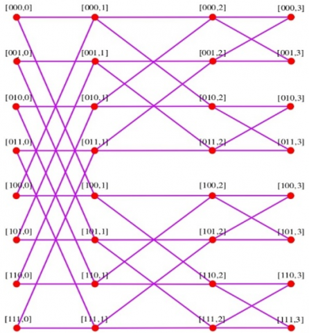
The butterfly network is a structured, multistage interconnection network widely used in parallel computing and digital signal processing, especially for executing the Fast Fourier Transform (FFT). Its recursive and hierarchical structure consists of $\text{lo}{{\text{g}}_{2}}n$ n stages for n inputs/outputs, where each node connects to two nodes in the next stage based on binary addressing see in the Figure 1. This fixed, regular pattern supports low-latency, deterministic routing, and scalability, making it ideal for systems with a large number of processors.
In applications such as supercomputing, telecommunications, and real-time signal processing, the butterfly network ensures fast and predictable data transfer. However, its main limitations are lack of fault tolerance and rigid routing paths, which can affect performance in dynamic environments. From a graph-theoretical view point, the butterfly network is modeled as a graph that is directed where nodes and edges represent switches and connections, respectively. We compute bond-additive molecular descriptors, specifically Adriatic indices, to quantify its topological structure [1-6].
Adriatic indices, degree-based graph invariants, quantify connectivity, redundancy, and network efficiency. In the butterfly network, they reveal how node degrees impact communication performance and structural strength. This study computes these indices to evaluate structural features, data transfer efficiency, and fault tolerance.
(a)
(b)
Figure 1. (a) Basic butterfly representation $F\left( 3 \right)$; (b) Diamond butterfly representation $BF\left( 3 \right)$
1.2 Benes network
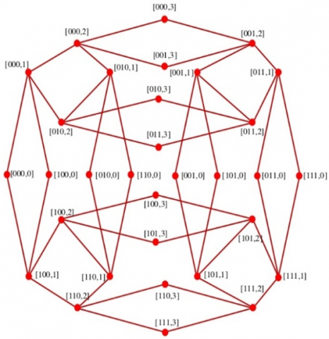
The benes network is a high-performance multistage interconnection topology widely used in parallel computing, optical switching, high-speed telecommunication, and large-scale data center networks. Structurally, it is constructed by connecting two mirror-image butterfly networks back-to-back, creating a symmetrical and rearrangeable non-blocking architecture in Figure 2. This arrangement enables permutation routing, allowing any input to connect to any output through multiple dynamically selectable paths.
(a)
(b)
Figure 2. (a) Basic benes network representation $N\left( 3 \right)$; (b) Diamond benes network representation $BN\left( 3 \right)$
For a network with n inputs/outputs, the Benes topology contains $2\text{lo}{{\text{g}}_{2}}n-1$ switching stages, each stage comprising switching nodes that route data according to binary-address-based connection rules. The central stage serves as a crossover layer, enabling efficient traffic rerouting. The network’s structural redundancy provides multiple alternative communication paths, ensuring fault tolerance, low congestion, and high throughput all essential in mission-critical applications such as real time signal processing and supercomputing.
From a graph theoretical standpoint, the benes network can be modeled as a multistage interconnection graph where vertices represent switching nodes and edges represent communication links. The degree of each node defined as the number of direct connections it holds is a fundamental parameter in analyzing the network’s structure. To evaluate and quantify the structural efficiency, connectivity, and robustness of the benes network, we apply Adriatic bond-additive molecular descriptors.
By computing Adriatic indices for the benes network, we aim to numerically evaluate its topological strength, compare it with other interconnection networks, and identify its suitability for large-scale, fault-tolerant computing systems.
1.3 Mesh derived networks
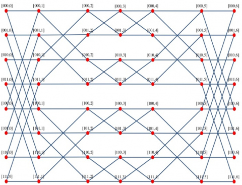
In parallel and distributed computing, mesh networks are a widely adopted topology due to their scalability, simplicity, and ability to deliver high data throughput with low latency. A conventional 2D mesh consists of nodes arranged in a grid pattern, where each node is connected to its immediate north, south, east, and west neighbors. While interior nodes have four connections, edge and corner nodes have fewer. The network diameter of a 2D mesh is $m+n-2$, representing the longest shortest path between any two nodes, and its bisection width is $\min \left( m,n \right)$, which indicates the potential for communication bottlenecks.
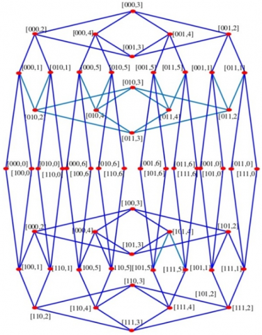
Despite their advantages, basic mesh networks face limitations such as relatively long path lengths, restricted fault tolerance, and inefficiencies in routing under high load. To address these issues, MDNs have been proposed. These networks modify the traditional mesh structure to enhance performance, scalability, and resilience. Common strategies include adding extra links, reconfiguring node connections, or integrating features from other topologies such as the Torus, Folded Mesh, or Crossed Mesh— each aiming to reduce latency, improve fault tolerance, or shorten the network diameter.
In this paper, we present two novel architectures:
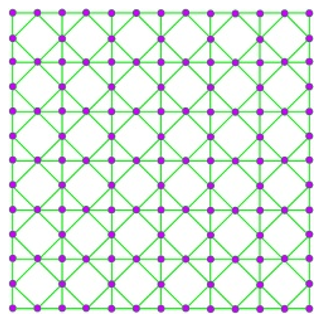
• $MD{{N}_{1}}\left( m,n \right)$ - based directly on the $m\times n$ mesh structure, modified to reduce communication distances and improve routing efficiency in Figure 3.
Figure 3. Mesh derived networks $MD{{N}_{1}}\left( 7,7 \right)$
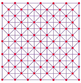
• $MD{{N}_{2}}\left( m,n \right)$ - derived by joining each vertex of a bounded dual $m+1\times n+1$ mesh to the corresponding face of the m×n mesh, creating additional connectivity and robustness in Figure 4.
Figure 4. Mesh derived networks $MD{{N}_{2}}\left( 7,7 \right)$
These enhancements aim to provide shorter communication paths, increased fault tolerance, and higher adaptability compared to the traditional mesh. We aim to analyze $MD{{N}_{1}}$ and $MD{{N}_{2}}$ using Adriatic indices, which are degree-based measures quantifying connectivity, redundancy, efficiency, and robustness. By applying these indices calculated through summing degree-based functions over all edges, we obtain a compact mathematical fingerprint of each network. This approach enables fast, simulation-free evaluation of structural complexity and performance, reveals the effect of link modifications on fault tolerance and communication efficiency, and allows benchmarking MDNs against other advanced interconnection networks for high-performance, fault-tolerant computing [7-15].
Let $G=\left( V\left( G \right),E\left( G \right) \right)$ be a graph. The cardinality of these collections symbolizes the no. of peaks and verges congruently. An edge in $E\left( G \right)$ through end-to-end vertices is signified by $e=uv$. Two vertices $u$ and $v$ supposed held to be organized if universally is a verge among them. The field of mathematical chemical science is a subfield of computational chemistry in which we use mathematical models to fight and predict the structure of molecules rather than relying on the laws of physics. A subfield of mathematical chemistry known as "chemical graph theory" applies graph theory to the mathematical demonstration of chemical occurrences [16-19]. The development of the biochemical sciences was greatly influenced by this notion.
A bond preservative descriptor Des can be inscribed as [20]:
$Des\left( G \right)=\underset{uv\in E\left( G \right)}{\mathop \sum }\,\text{}f\left( {{d}_{G}}\left( u \right),{{d}_{G}}\left( v \right) \right)$
where, $E\left( G \right)$ is the established of edges and $f$ is around charting that allocates an actual value to a well-ordered pair containing of a structure and it is an edge. It can be understood that this stands a fairly overall meaning since $f$ can be single-minded in many customs.
The topological indices described above are a collection of molecular descriptors used to quantify the structural characteristics of molecules. Each index is calculated based on the degrees (or valences) of atoms in a molecular graph, denoted as ${{d}_{u}}$ and ${{d}_{v}}$ for two adjacent atoms $u$ and $v$.
The 15 Adriatic index formulas are divided into three main types. The logarithmic-based indices help detect small, hidden changes in network connectivity and identify weak points that could slow communication. The imbalance-based indices measure differences in how nodes are connected, which helps evaluate whether the network is balanced, strong, and resistant to failures. The ratio-based indices compare connection proportions to see if the network is evenly connected or follows a hub-spoke pattern. Together, these formulas provide a simple, calculation-based way to study, compare, and improve networks like Butterfly, Benes, and MDNs.
a. Randic-type Lordeg index: This index is derived from the product of the natural logarithms of the degrees of adjacent atoms, $\ln \left( {{d}_{u}} \right)\times \ln \left( {{d}_{v}} \right)$. It captures the local structural properties of molecules and is sensitive to variations in atom degrees.
b. Sum Lordeg index: This index is calculated as the sum of the square roots of the natural logarithms of the degrees of adjacent atoms, $\sqrt{\ln \left( {{d}_{u}} \right)}+\sqrt{\ln \left( {{d}_{v}} \right)}$. It provides a measure of overall structural complexity and connectivity in a molecule.
c. Inverse sum Lordeg index: The reciprocal of the sum Lordeg index, $\frac{1}{\sqrt{\ln \left( {{d}_{u}} \right)}+\sqrt{\ln \left( {{d}_{v}} \right)}}$, observation into the inverse connection between structural complexity and connectivity.
d. Misbalance Lordeg index: This index calculates the complete variation between the natural logarithms of the degrees of adjacent atoms, $\left| \ln \left( {{d}_{u}} \right)-\ln \left( {{d}_{v}} \right) \right|$. It computes the degree of imbalance.
e. Misbalance Losdeg index: Similar to the misbalance Lordeg index, but using squared natural logarithms of degrees, $\left| l{{n}^{2}}{{d}_{u}}-l{{n}^{2}}{{d}_{v}} \right|$. It emphasizes larger differences in connectivity.
f. Misbalance Indeg index: This index computes the absolute difference between the reciprocals of degrees of adjacent atoms, $\left| \frac{1}{{{d}_{u}}}-\frac{1}{{{d}_{v}}} \right|$. It focuses on disparities in atom valences.
g. Misbalance Irdeg index: Similar to the misbalance Indeg index, but using the reciprocals of the square roots of degrees, $\left| \frac{1}{\sqrt{{{d}_{u}}}}-\frac{1}{\sqrt{{{d}_{v}}}} \right|$. It emphasizes differences in valences while considering structural complexity.
h. Misbalance Rodeg index: This index measures the absolute difference between the square roots of degrees of adjacent atoms, $\left| \sqrt{{{d}_{u}}}-\sqrt{{{d}_{v}}} \right|$. It captures differences in connectivity, giving more weight to atoms with higher degrees.
i. Misbalance deg index: The absolute difference between the degrees of adjacent atoms, $\left| {{d}_{u}}-{{d}_{v}} \right|$, quantifies variations in atom valences.
j. Misbalance Hadeg index: This index measures the absolute difference between the halves of the degrees of adjacent atoms, $\left| {{\left( \frac{1}{2} \right)}^{{{d}_{u}}}}-{{\left( \frac{1}{2} \right)}^{{{d}_{v}}}} \right|$. It emphasizes differences in connectivity while considering the magnitude of degrees.
k. Minimum-maxi Rodeg index: This index is the square root of the ratio of the smaller to the larger degree of adjacent atoms, $\sqrt{\frac{\min \left( {{d}_{u}},{{d}_{v}} \right)}{\max \left( {{d}_{u}},{{d}_{v}} \right)}}$. It highlights the relative degree discrepancy between adjacent atoms.
l. Max-Minirodeg index: The square root of the ratio of the larger to the smaller degree of adjacent atoms, $\sqrt{\frac{\max \left( {{d}_{u}},{{d}_{v}} \right)}{\min \left( {{d}_{u}},{{d}_{v}} \right)}}$, emphasizes the relative degree discrepancy in the opposite direction.
m. Max-Minideg index: The ratio of the larger to the smaller degree of adjacent atoms, $\frac{\max \left( {{d}_{u}},{{d}_{v}} \right)}{\min \left( {{d}_{u}},{{d}_{v}} \right)}$, quantifies the relative degree discrepancy without square rooting.
n. Max-Minisdeg index: The square of the max-Minideg index, ${{\left( \frac{\max \left( {{d}_{u}},{{d}_{v}} \right)}{\min \left( {{d}_{u}},{{d}_{v}} \right)} \right)}^{2}}$, amplifies the effect of degree discrepancy, emphasizing larger differences.
o. Symmetric division deg index: This index is the sum of the reciprocal of the smaller to larger degree ratio and the reciprocal of the larger to smaller degree ratio, $\frac{\min \left( {{d}_{u}},{{d}_{v}} \right)}{\max \left( {{d}_{u}},{{d}_{v}} \right)}+\frac{\max \left( {{d}_{u}},{{d}_{v}} \right)}{\min \left( {{d}_{u}},{{d}_{v}} \right)}$. It provides a balanced measure of relative degree discrepancy between adjacent atoms.
We use Adriatic index formulas for butterfly, benes, and MDNs because they convert complex topological properties - connectivity, fault tolerance, efficiency, and hierarchy-into precise numerical values. This allows direct, simulation-free comparison of communication performance, robustness, and structural optimization potential across all three network types.
Topological indices are the appreciated tools providing by the graph theory for theoretical learn of material compounds [21-33].
Let $G$ be the butterfly network of dimension $n$. The number of vertices and edges in BF(n) are ${{2}^{n}}\left( n+1 \right)$ and $n{{2}^{n+1}}$ respectively see Figure 1. The edge partition and the end vertex degree sum are presented in see Table 1.
Table 1. The edge partition of butterfly network BF(n)
|
$\left( {{d}_{u}},{{d}_{v}} \right)$ |
No. of Edges |
|
(2,4) |
${{2}^{n+2}}$ |
|
(4,4) |
${{2}^{n+1}}\left( n-2 \right)$ |
|
Theorem 1. Let G be a butterfly network BF(n), then |
|
1. $RLI\left( G \right)=0.9608\times {{2}^{n+2}}+1.9218n\times {{2}^{n+1}}-$ $\text{ }\!\!~\!\!\text{ }\!\!~\!\!\text{ }\!\!~\!\!\text{ }\!\!~\!\!\text{ }\!\!~\!\!\text{ }\!\!~\!\!\text{ }\!\!~\!\!\text{ }\!\!~\!\!\text{ }\!\!~\!\!\text{ }3.8437\times {{2}^{n+1}}$. 2. $SLI\left( G \right)=2.0099\times {{2}^{n+2}}+2.3548n\times {{2}^{n+1}}-4.7096\times {{2}^{n+1}}$. 3. $ISLI\left( G \right)=0.4975\times {{2}^{n+2}}+0.4247\times {{2}^{n+1}}\left( n-2 \right)$. 4. $MLI\left( G \right)=0.6932\times {{2}^{n+2}}$. 5. $MLSI\left( G \right)=1.4413\times {{2}^{n+2}}$. 6. $MII\left( G \right)={{2}^{n}}$. 7. $MIRI\left( G \right)=0.2071\times {{2}^{n+2}}$. 8. $MRI\left( G \right)=0.5858\times {{2}^{n+2}}$. 9. $MDI\left( G \right)={{2}^{n+3}}$. 10. $MHI\left( G \right)=0.1875\times {{2}^{n+2}}$. 11. $MMRI\left( G \right)=-0.2929\times {{2}^{n+2}}+n\times {{2}^{n+1}}$. 12. $MMRDI\left( G \right)=0.414\times {{2}^{n+2}}+n\times {{2}^{n+1}}$. 13. $MMDI\left( G \right)={{2}^{n+3}}+{{2}^{n+1}}\left( n-2 \right)$. 14. $MMSDI\left( G \right)={{2}^{n+4}}+{{2}^{n+1}}\left( n-2 \right)$. 15. $SDDI\left( G \right)=2.5\times {{2}^{n+2}}+{{2}^{n+2}}\left( n-2 \right)$. |
Proof.
Using the vertex degree pairings (2,4) and (4,4) and the two edge partitions $\left( {{2}^{n+2}},{{2}^{n+1}}\left( n-2 \right) \right)$, all 15 indices for BF(n) are clearly obtained in this theorem, producing precise results for each index based on edge-vertex features.
$RLI\left( G \right)=\underset{uv\in E\left( G \right)}{\mathop \sum }\,\text{}ln{{d}_{G}}\left( u \right)ln{{d}_{G}}\left( v \right) =\left( ln2\times ln4 \right)\left( {{2}^{n+2}} \right)+\left( ln4\times ln4 \right)\left( {{2}^{n+1}}\left( n-2 \right) \right)=0.9608\times {{2}^{n+2}}+1.9218n\times {{2}^{n+1}}-3.8437\times {{2}^{n+1}}$
$SLI\left( G \right)=\underset{uv\in E\left( G \right)}{\mathop \sum }\,\text{}\sqrt{\ln \left( {{d}_{u}} \right)}+\sqrt{\ln \left( {{d}_{v}} \right)}$
$=\left[ \sqrt{\ln \left( 2 \right)}+\sqrt{\ln \left( 4 \right)} \right]\left( {{2}^{n+2}} \right)+\left[ \sqrt{\ln \left( 4 \right)}+\sqrt{\ln \left( 4 \right)} \right]\left( {{2}^{n+1}}\left( n-2 \right) \right)$
$=2.0099\times {{2}^{n+2}}+2.3548n\times {{2}^{n+1}}-4.7096\times {{2}^{n+1}}$
$ISLI\left( G \right)=\underset{uv\in E\left( G \right)}{\mathop \sum }\,\text{}\frac{1}{\sqrt{\ln \left( {{d}_{u}} \right)}+\sqrt{\ln \left( {{d}_{v}} \right)}}=\left[ \frac{1}{\sqrt{\ln \left( 2 \right)}+\sqrt{\ln \left( 4 \right)}} \right]\left( {{2}^{n+2}} \right)+\left[ \frac{1}{\sqrt{\ln \left( 4 \right)}+\sqrt{\ln \left( 4 \right)}} \right]\left( {{2}^{n+1}}\left( n-2 \right) \right)=0.4975\times {{2}^{n+2}}+0.4247\times {{2}^{n+1}}\left( n-2 \right)$
$MLI\left( G \right)=\underset{uv\in E\left( G \right)}{\mathop \sum }\,\text{}\left| ln{{d}_{u}}-ln{{d}_{v}} \right|$ $=\left| ln2-ln4 \right|\left( {{2}^{n+2}} \right)+\left| ln4-ln4 \right|\left( {{2}^{n+1}}\left( n-2 \right) \right)=0.6932\times {{2}^{n+2}}$
$MLSI\left( G \right)=\underset{uv\in E\left( G \right)}{\mathop \sum }\,\text{}\left| l{{n}^{2}}{{d}_{u}}-l{{n}^{2}}{{d}_{v}} \right|=\left| l{{n}^{2}}2-l{{n}^{2}}4 \right|\left( {{2}^{n+2}} \right)+\left| l{{n}^{2}}4-l{{n}^{2}}4 \right|\left( {{2}^{n+1}}\left( n-2 \right) \right) =1.4413\times {{2}^{n+2}}$
$MII\left( G \right)=\underset{uv\in E\left( G \right)}{\mathop \sum }\,\text{}\left| \frac{1}{{{d}_{u}}}-\frac{1}{{{d}_{v}}} \right|=\left| \frac{1}{2}-\frac{1}{4} \right|\left( {{2}^{n+2}} \right)+\left| \frac{1}{4}-\frac{1}{4} \right|\left( {{2}^{n+1}}\left( n-2 \right) \right)$ $={{2}^{n}}$
$MIRI\left( G \right)=\underset{uv\in E\left( G \right)}{\mathop \sum }\,\text{}\left| \frac{1}{\sqrt{{{d}_{u}}}}-\frac{1}{\sqrt{{{d}_{v}}}} \right|=\left| \frac{1}{\sqrt{2}}-\frac{1}{\sqrt{4}} \right|\left( {{2}^{n+2}} \right)$ $+\left| \frac{1}{\sqrt{4}}-\frac{1}{\sqrt{4}} \right|\left( {{2}^{n+1}}\left( n-2 \right) \right)=0.2071\times {{2}^{n+2}}$
$MRI\left( G \right)=\underset{uv\in E\left( G \right)}{\mathop \sum }\,\text{}\left| \sqrt{{{d}_{u}}}-\sqrt{{{d}_{v}}} \right|=\left| \sqrt{2}-\sqrt{4} \right|\left( {{2}^{n+2}} \right)$ $+\left| \sqrt{4}-\sqrt{4} \right|\left( {{2}^{n+1}}\left( n-2 \right) \right)=0.5858\times {{2}^{n+2}}$
$MDI\left( G \right)=\underset{uv\in E\left( G \right)}{\mathop \sum }\,\text{}\left| {{d}_{u}}-{{d}_{v}} \right|=\left| 2-4 \right|\left( {{2}^{n+2}} \right)+\left| 4-4 \right|\left( {{2}^{n+1}}\left( n-2 \right) \right)={{2}^{n+3}}$
$MHI\left( G \right)=\underset{uv\in E\left( G \right)}{\mathop \sum }\,\text{}\left| {{\left( \frac{1}{2} \right)}^{{{d}_{u}}}}-{{\left( \frac{1}{2} \right)}^{{{d}_{v}}}} \right|=\left| {{\left( \frac{1}{2} \right)}^{2}}-{{\left( \frac{1}{2} \right)}^{4}} \right|\left( {{2}^{n+2}} \right)$ $+\left| {{\left( \frac{1}{2} \right)}^{4}}-{{\left( \frac{1}{2} \right)}^{4}} \right|\left( {{2}^{n+1}}\left( n-2 \right) \right)=0.1875\times {{2}^{n+2}}$
$MMRI\left( G \right)=\underset{uv\in E\left( G \right)}{\mathop \sum }\,\text{}\sqrt{\frac{mini\left( {{d}_{u}},{{d}_{v}} \right)}{maxi\left( {{d}_{u}},{{d}_{v}} \right)}}=\sqrt{\frac{mini\left( 2,4 \right)}{maxi\left( 2,4 \right)}}\left( {{2}^{n+2}} \right)$ $+\sqrt{\frac{mini\left( 4,4 \right)}{maxi\left( 4,4 \right)}}\left( {{2}^{n+1}}\left( n-2 \right) \right)=-0.2929\times {{2}^{n+2}}+n\times {{2}^{n+1}}$
$MMRDI\left( G \right)=\underset{uv\in E\left( G \right)}{\mathop \sum }\,\text{}\sqrt{\frac{maxi\left( {{d}_{u}},{{d}_{v}} \right)}{mini\left( {{d}_{u}},{{d}_{v}} \right)}}=\sqrt{\frac{maxi\left( 2,4 \right)}{mini\left( 2,4 \right)}}\left( {{2}^{n+2}} \right)+\sqrt{\frac{maxi\left( 4,4 \right)}{mini\left( 4,4 \right)}}\left( {{2}^{n+1}}\left( n-2 \right) \right)=0.414\times {{2}^{n+2}}+n\times {{2}^{n+1}}$
$MMDI\left( G \right)=\underset{uv\in E\left( G \right)}{\mathop \sum }\,\text{}\frac{maxi\left( {{d}_{u}},{{d}_{v}} \right)}{mini\left( {{d}_{u}},{{d}_{v}} \right)}=\frac{maxi\left( 2,4 \right)}{mini\left( 2,4 \right)}\left( {{2}^{n+2}} \right)+\frac{maxi\left( 4,4 \right)}{mini\left( 4,4 \right)}\left( {{2}^{n+1}}\left( n-2 \right) \right)={{2}^{n+3}}+{{2}^{n+1}}\left( n-2 \right)$
$MMSDI\left( G \right)=\underset{uv\in E\left( G \right)}{\mathop \sum }\,\text{}{{\left( \frac{maxi\left( {{d}_{u}},{{d}_{v}} \right)}{mini\left( {{d}_{u}},{{d}_{v}} \right)} \right)}^{2}}={{\left( \frac{maxi\left( 2,4 \right)}{mini\left( 2,4 \right)} \right)}^{2}}\left( {{2}^{n+2}} \right)+{{\left( \frac{maxi\left( 4,4 \right)}{mini\left( 4,4 \right)} \right)}^{2}}\left( {{2}^{n+1}}\left( n-2 \right) \right)={{2}^{n+4}}+{{2}^{n+1}}\left( n-2 \right)$
$SDDI\left( G \right)=\underset{uv\in E\left( G \right)}{\mathop \sum }\,\text{}\left[ \frac{mini\left( {{d}_{u}},{{d}_{v}} \right)}{maxi\left( {{d}_{u}},{{d}_{v}} \right)}+\frac{maxi\left( {{d}_{u}},{{d}_{v}} \right)}{mini\left( {{d}_{u}},{{d}_{v}} \right)} \right]=\left[ \frac{\text{mini}\left( 2,4 \right)}{\max i\left( 2,4 \right)}+\frac{\max i\left( 2,4 \right)}{\text{mini}\left( 2,4 \right)} \right]\left( {{2}^{n+2}} \right)+\left[ \frac{mini\left( 4,4 \right)}{maxi\left( 4,4 \right)}+\frac{maxi\left( 4,4 \right)}{mini\left( 4,4 \right)} \right]\left( {{2}^{n+1}}\left( n-2 \right) \right)=2.5\times {{2}^{n+2}}+{{2}^{n+2}}\left( n-2 \right)$
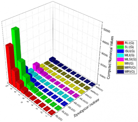
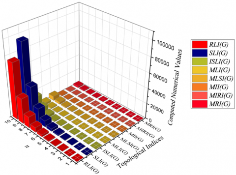
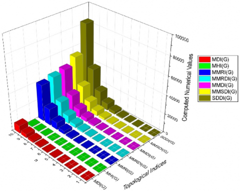
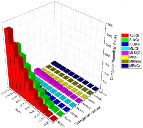
The numerical values are presented in Table 2 and graphical representations of various bond-additive molecular descriptors for butterfly network $BF\left( n \right)$ structures are presented in Figure 5.
Table 2. Calculated bond additive numerical value
|
$n$ |
$RLI(G)$ |
$SLI\left( G \right)$ |
$ISLI\left( G \right)$ |
$MLI\left( G \right)$ |
$MLSI\left( G \right)$ |
$MII\left( G \right)$ |
$MIRI\left( G \right)$ |
$MRI\left( G \right)$ |
|
1 |
0 |
7 |
2 |
6 |
12 |
2 |
2 |
5 |
|
2 |
15 |
32 |
8 |
11 |
23 |
4 |
3 |
9 |
|
3 |
61 |
102 |
23 |
22 |
46 |
8 |
7 |
19 |
|
4 |
184 |
279 |
59 |
44 |
92 |
16 |
13 |
37 |
|
5 |
492 |
709 |
145 |
89 |
184 |
32 |
27 |
75 |
|
6 |
1230 |
1720 |
345 |
177 |
369 |
64 |
53 |
150 |
|
7 |
2952 |
4043 |
798 |
355 |
738 |
128 |
106 |
300 |
|
8 |
6888 |
9292 |
1814 |
710 |
1476 |
256 |
212 |
600 |
|
9 |
15743 |
20995 |
4063 |
1420 |
2952 |
512 |
424 |
1200 |
|
10 |
35422 |
46814 |
8996 |
2839 |
5904 |
1024 |
848 |
2399 |
|
$n$ |
$MDI\left( G \right)$ |
$MHI\left( G \right)$ |
$MMRI\left( G \right)$ |
$MMRDI\left( G \right)$ |
$MMDI\left( G \right)$ |
$MMSDI\left( G \right)$ |
$SDDI\left( G \right)$ |
|
|
1 |
16 |
2 |
2 |
7 |
12 |
28 |
12 |
|
|
2 |
32 |
3 |
11 |
23 |
32 |
64 |
40 |
|
|
3 |
64 |
6 |
39 |
61 |
80 |
144 |
112 |
|
|
4 |
128 |
12 |
109 |
154 |
192 |
320 |
288 |
|
|
5 |
256 |
24 |
283 |
373 |
448 |
704 |
704 |
|
|
6 |
512 |
48 |
693 |
874 |
1024 |
1536 |
1664 |
|
|
7 |
1024 |
96 |
1642 |
2004 |
2304 |
3328 |
3840 |
|
|
8 |
2048 |
192 |
3796 |
4520 |
5120 |
7168 |
8704 |
|
|
9 |
4096 |
384 |
8616 |
10064 |
11264 |
15360 |
19456 |
|
|
10 |
8192 |
768 |
19280 |
22176 |
24576 |
32768 |
43008 |
|
(a)
(b)
Figure 5. A visual representation of molecular characteristics for bond addition of butterfly network $BF\left( n \right)$
Assume that $G$ is the benes network of size $n$. We obtained a generalized structure with ${{2}^{n}}\left( 2n+1 \right)$ vertices and $n{{2}^{n+2}}$ edges from the benes network. In Table 3, the pertinent edge partition is shown.
Table 3. The benes network’s edge segment
|
$\left( {{d}_{u}},{{d}_{v}} \right)$ |
No. of Edges |
|
(2,4) |
${{2}^{n+2}}$ |
|
(4,4) |
${{2}^{n+2}}\left( n-1 \right)$ |
|
Theorem 2. Consider a benes network G, then |
|
1. $RLI\left( G \right)=-0.9610\times {{2}^{n+2}}+1.9218n\times {{2}^{n+2}}$. 2. $SLI\left( G \right)=-0.3449\times {{2}^{n+2}}+2.3548n\times {{2}^{n+2}}$. 3. $ISLI\left( G \right)=0.42466\times {{2}^{n+2}}n+0.07287\times {{2}^{n+2}}$. 4. $MLI\left( G \right)=0.6932\times {{2}^{n+2}}$. 5. $MLSI\left( G \right)=1.4413\times {{2}^{n+2}}$. 6. $MII\left( G \right)={{2}^{n}}$. 7. $MIRI\left( G \right)=0.2071\times {{2}^{n+2}}$. 8. $MRI\left( G \right)=0.5858\times {{2}^{n+2}}$ 9. $MDI\left( G \right)={{2}^{n+3}}$. 10. $MHI\left( G \right)=0.1875\times {{2}^{n+2}}$. 11. $MMRI\left( G \right)=-0.2929\times {{2}^{n+2}}+n\times {{2}^{n+2}}$. 12. $MMRDI\left( G \right)=0.4142\times {{2}^{n+2}}+n\times {{2}^{n+2}}$. 13. $MMDI\left( G \right)={{2}^{n+3}}+{{2}^{n+2}}\left( n-1 \right)$. 14. $MMSDI\left( G \right)={{2}^{n+4}}+{{2}^{n+2}}\left( n-1 \right)$. 15. $SDDI\left( G \right)=2.5\times {{2}^{n+2}}+{{2}^{n+3}}\left( n-1 \right)$. |
Proof.
In this theorem, all 15 indices for $B\left( n \right)$ are clearly derived using the vertex degree pairs (2,4) and (4,4) and the two edge partitions $({{2}^{n+2}},~{{2}^{n+2}}\left( n-1 \right))$. Based on edge-vertex characteristics, this theorem yields exact results for each index.
$RLI\left( G \right)=\underset{uv\in E\left( G \right)}{\mathop \sum }\,\text{}ln{{d}_{G}}\left( u \right)ln{{d}_{G}}\left( v \right)=\left( ln2\times ln4 \right)\left( {{2}^{n+2}} \right)+\left( ln4\times ln4 \right)\left( {{2}^{n+2}}\left( n-1 \right) \right)=-0.9610\times {{2}^{n+2}}+{{1.9218\times2}^{n+2}}$
$SLI\left( G \right)=\underset{uv\in E\left( G \right)}{\mathop \sum }\,\text{}\sqrt{\ln \left( {{d}_{u}} \right)}+\sqrt{\ln \left( {{d}_{v}} \right)}=\left[ \sqrt{\ln \left( 2 \right)}+\sqrt{\ln \left( 4 \right)} \right]\left( {{2}^{n+2}} \right)+\left[ \sqrt{\ln \left( 4 \right)}+\sqrt{\ln \left( 4 \right)} \right]\left( {{2}^{n+2}}\left( n-1 \right) \right)=-0.3449\times {{2}^{n+2}}+2.3548n\times {{2}^{n+2}}$
$ISLI\left( G \right)=\underset{uv\in E\left( G \right)}{\mathop \sum }\,\text{}\frac{1}{\sqrt{\ln \left( {{d}_{u}} \right)}+\sqrt{\ln \left( {{d}_{v}} \right)}}=\left[ \frac{1}{\sqrt{\ln \left( 2 \right)}+\sqrt{\ln \left( 4 \right)}} \right]\left( {{2}^{n+2}} \right)+\left[ \frac{1}{\sqrt{\ln \left( 4 \right)}+\sqrt{\ln \left( 4 \right)}} \right]\left( {{2}^{n+2}}\left( n-1 \right) \right)=0.42466\times {{2}^{n+2}}n+0.07287\times {{2}^{n+2}}$
$MLI\left( G \right)=\underset{uv\in E\left( G \right)}{\mathop \sum }\,\text{}\left| ln{{d}_{u}}-ln{{d}_{v}} \right|=\left| ln2-ln4 \right|\left( {{2}^{n+2}} \right)+\left| ln4-ln4 \right|\left( {{2}^{n+2}}\left( n-1 \right) \right)=0.6932\times {{2}^{n+2}}$
$MLSI\left( G \right)=\underset{uv\in E\left( G \right)}{\mathop \sum }\,\text{}\left| l{{n}^{2}}{{d}_{u}}-l{{n}^{2}}{{d}_{v}} \right|=\left| l{{n}^{2}}2-l{{n}^{2}}4 \right|\left( {{2}^{n+2}} \right)+\left| l{{n}^{2}}4-l{{n}^{2}}4 \right|\left( {{2}^{n+2}}\left( n-1 \right) \right)=1.4413\times {{2}^{n+2}}$
$MII\left( G \right)=\underset{uv\in E\left( G \right)}{\mathop \sum }\,\text{}\left| \frac{1}{{{d}_{u}}}-\frac{1}{{{d}_{v}}} \right|=\left| \frac{1}{2}-\frac{1}{4} \right|\left( {{2}^{n+2}} \right)+\left| \frac{1}{4}-\frac{1}{4} \right|\left( {{2}^{n+2}}\left( n-1 \right) \right)={{2}^{n}}$
$MIRI\left( G \right)=\underset{uv\in E\left( G \right)}{\mathop \sum }\,\text{}\left| \frac{1}{\sqrt{{{d}_{u}}}}-\frac{1}{\sqrt{{{d}_{v}}}} \right|=\left| \frac{1}{\sqrt{2}}-\frac{1}{\sqrt{4}} \right|\left( {{2}^{n+2}} \right)+\left| \frac{1}{\sqrt{4}}-\frac{1}{\sqrt{4}} \right|\left( {{2}^{n+2}}\left( n-1 \right) \right)=0.2071\times {{2}^{n+2}}$
$MRI\left( G \right)=\underset{uv\in E\left( G \right)}{\mathop \sum }\,\text{}\left| \sqrt{{{d}_{u}}}-\sqrt{{{d}_{v}}} \right|=\left| \sqrt{2}-\sqrt{4} \right|\left( {{2}^{n+2}} \right)+\left| \sqrt{4}-\sqrt{4} \right|\left( {{2}^{n+2}}\left( n-1 \right) \right)=0.5858\times {{2}^{n+2}}$
$MDI\left( G \right)=\underset{uv\in E\left( G \right)}{\mathop \sum }\,\text{}\left| {{d}_{u}}-{{d}_{v}} \right|=\left| 2-4 \right|\left( {{2}^{n+2}} \right)+\left| 4-4 \right|\left( {{2}^{n+2}}\left( n-1 \right) \right) ={{2}^{n+3}}$
$MHI\left( G \right)=\underset{uv\in E\left( G \right)}{\mathop \sum }\,\text{}\left| {{\left( \frac{1}{2} \right)}^{{{d}_{u}}}}-{{\left( \frac{1}{2} \right)}^{{{d}_{v}}}} \right|=\left| {{\left( \frac{1}{2} \right)}^{2}}-{{\left( \frac{1}{2} \right)}^{4}} \right|\left( {{2}^{n+2}} \right)+\left| {{\left( \frac{1}{2} \right)}^{4}}-{{\left( \frac{1}{2} \right)}^{4}} \right|\left( {{2}^{n+2}}\left( n-1 \right) \right)=0.1875\times {{2}^{n+2}}$
$MMRI\left( G \right)=\underset{uv\in E\left( G \right)}{\mathop \sum }\,\text{}\sqrt{\frac{mini\left( {{d}_{u}},{{d}_{v}} \right)}{maxi\left( {{d}_{u}},{{d}_{v}} \right)}}=\sqrt{\frac{mini\left( 2,4 \right)}{maxi\left( 2,4 \right)}}\left( {{2}^{n+2}} \right)+\sqrt{\frac{mini\left( 4,4 \right)}{maxi\left( 4,4 \right)}}\left( {{2}^{n+2}}\left( n-1 \right) \right)=-0.2929\times {{2}^{n+2}}+n\times {{2}^{n+2}}$
$MMRDI\left( G \right)=\underset{uv\in E\left( G \right)}{\mathop \sum }\,\text{}\sqrt{\frac{maxi\left( {{d}_{u}},{{d}_{v}} \right)}{mini\left( {{d}_{u}},{{d}_{v}} \right)}}=\sqrt{\frac{maxi\left( 2,4 \right)}{mini\left( 2,4 \right)}}\left( {{2}^{n+2}} \right)+\sqrt{\frac{maxi\left( 4,4 \right)}{mini\left( 4,4 \right)}}\left( {{2}^{n+2}}\left( n-1 \right) \right)=0.414\times {{2}^{n+2}}+n\times {{2}^{n+1}}$
$MMDI\left( G \right)=\underset{uv\in E\left( G \right)}{\mathop \sum }\,\text{}\frac{maxi\left( {{d}_{u}},{{d}_{v}} \right)}{mini\left( {{d}_{u}},{{d}_{v}} \right)}=\frac{maxi\left( 2,4 \right)}{mini\left( 2,4 \right)}\left( {{2}^{n+2}} \right)+\frac{maxi\left( 4,4 \right)}{mini\left( 4,4 \right)}\left( {{2}^{n+2}}\left( n-1 \right) \right)={{2}^{n+3}}+{{2}^{n+2}}\left( n-1 \right)$
$MMSDI\left( G \right)=\underset{uv\in E\left( G \right)}{\mathop \sum }\,\text{}{{\left( \frac{maxi\left( {{d}_{u}},{{d}_{v}} \right)}{mini\left( {{d}_{u}},{{d}_{v}} \right)} \right)}^{2}}={{\left( \frac{maxi\left( 2,4 \right)}{mini\left( 2,4 \right)} \right)}^{2}}\left( {{2}^{n+2}} \right)+{{\left( \frac{maxi\left( 4,4 \right)}{mini\left( 4,4 \right)} \right)}^{2}}\left( {{2}^{n+2}}\left( n-1 \right) \right)={{2}^{n+4}}+{{2}^{n+2}}\left( n-1 \right)$
$SDDI\left( G \right)=\underset{uv\in E\left( G \right)}{\mathop \sum }\,\text{}\left[ \frac{mini\left( {{d}_{u}},{{d}_{v}} \right)}{maxi\left( {{d}_{u}},{{d}_{v}} \right)}+\frac{maxi\left( {{d}_{u}},{{d}_{v}} \right)}{mini\left( {{d}_{u}},{{d}_{v}} \right)} \right]=\left[ \frac{\text{mini}\left( 2,4 \right)}{\text{maxi}\left( 2,4 \right)}+\frac{\max i\left( 2,4 \right)}{\min i\left( 2,4 \right)} \right]\left( {{2}^{n+2}} \right)+\left[ \frac{\text{mini}\left( 4,4 \right)}{\max i\left( 4,4 \right)}+\frac{\max i\left( 4,4 \right)}{\min i\left( 4,4 \right)} \right]\left( {{2}^{n+2}}\left( n-1 \right) \right)=2.5\times {{2}^{n+2}}+{{2}^{n+3}}\left( n-1 \right)$
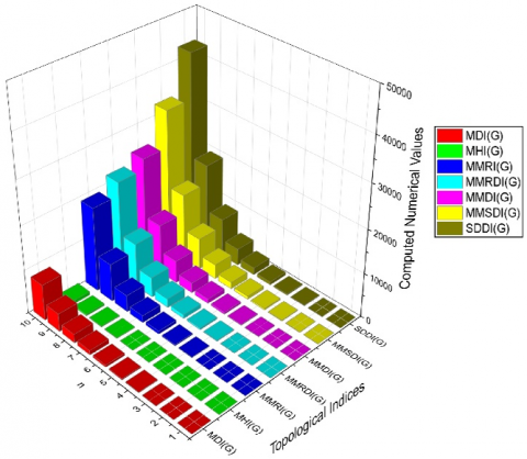
The numerical values are presented in Table 4 and graphical representations of various bond-additive molecular descriptors for Benes Network structures are presented in Figure 6.
Table 4. Calculated bond additive numerical value
|
$n$ |
$RLI\left( G \right)$ |
$SLI\left( G \right)$ |
$ISLI\left( G \right)$ |
$MLI\left( G \right)$ |
$MLSI\left( G \right)$ |
$MII\left( G \right)$ |
$MIRI\left( G \right)$ |
$MRI\left( G \right)$ |
|
1 |
8 |
16 |
4 |
6 |
12 |
2 |
2 |
5 |
|
2 |
46 |
70 |
15 |
11 |
23 |
4 |
3 |
9 |
|
3 |
154 |
215 |
43 |
22 |
46 |
8 |
7 |
19 |
|
4 |
430 |
581 |
113 |
44 |
92 |
16 |
13 |
37 |
|
5 |
1107 |
1463 |
281 |
89 |
184 |
32 |
27 |
75 |
|
6 |
2706 |
3529 |
671 |
177 |
369 |
64 |
53 |
150 |
|
7 |
6396 |
8263 |
1559 |
355 |
738 |
128 |
106 |
300 |
|
8 |
14759 |
18937 |
3553 |
710 |
1476 |
256 |
212 |
600 |
|
9 |
33454 |
42697 |
7977 |
1420 |
2952 |
512 |
424 |
1200 |
|
10 |
74781 |
95040 |
17693 |
2839 |
5904 |
1024 |
848 |
2399 |
|
$n$ |
$MDI\left( G \right)$ |
$MHI\left( G \right)$ |
$MMRI\left( G \right)$ |
$MMRDI\left( G \right)$ |
$MMDI\left( G \right)$ |
$MMSDI\left( G \right)$ |
$SDDI\left( G \right)$ |
|
|
1 |
16 |
2 |
6 |
11 |
16 |
32 |
20 |
|
|
2 |
32 |
3 |
27 |
39 |
48 |
80 |
72 |
|
|
3 |
64 |
6 |
87 |
109 |
128 |
192 |
208 |
|
|
4 |
128 |
12 |
237 |
283 |
320 |
448 |
544 |
|
|
5 |
256 |
24 |
603 |
693 |
768 |
1024 |
1344 |
|
|
6 |
512 |
48 |
1461 |
1642 |
1792 |
2304 |
3200 |
|
|
7 |
1024 |
96 |
3434 |
3796 |
4096 |
5120 |
7424 |
|
|
8 |
2048 |
192 |
7892 |
8616 |
9216 |
11264 |
16896 |
|
|
9 |
4096 |
384 |
17832 |
19280 |
20480 |
24576 |
37888 |
|
|
10 |
8192 |
768 |
39760 |
42657 |
45056 |
53248 |
83968 |
|
(a)
(b)
Figure 6. A visual representation of molecular characteristics for bond addition of benes network
Let $G$ be the $MD{{N}_{1}}\left( m,n \right)$ network, where $m$ and $n$ are its defining parameters. In $MD{{N}_{1}}\left( m,n \right)$, there are $3mn-m-n$ vertices and $8mn-6\left( m+n \right)+4$ edges, respectively. The Table 5 provides the edge partition and the end vertex degree sum.
Table 5. Mesh derived network $MD{{N}_{1}}\left( m,n \right)$
|
$\left( {{d}_{u}},{{d}_{v}} \right)$ |
No. of Edges |
|
(2,4) |
$8$ |
|
(3,4) |
$4\left( m+n-4 \right)$ |
|
(3,6) |
$2\left( m+n-4 \right)$ |
|
(4,4) |
$4$ |
|
(4,6) |
$4\left( mn-m-n \right)$ |
|
(6,6) |
$4\left( mn-2m-2n+4 \right)$ |
|
Theorem 3. Let G be a mesh derived network $\text{MD}{{\text{N}}_{1}}\left( \text{m},\text{n} \right)$, then |
|
1. $RLI\left( G \right)=22.7780mn-25.5914m-25.5914n+26.6272$. 2. $SLI\left( G \right)=20.7728mn-17.8062m-17.8062n+13.632$. 3.$ISLI\left( G \right)=3.0839mn-1.9427m-1.9427n+1.1140$. 4. $MLI(G) = 1.5955m^{2} + 1.5955n^{2} + 4.8129mn \\\quad - 14.3858m - 14.3858n + 31.0731$. 5. $MLSI\left( G \right)=3.2436mn+1.8306m+1.8306n -9.2064$. 6. $MII\left( G \right)=\left( m+n+mn-2 \right)/3$. 7. $MIRI\left( G \right)=0.3670mn+0.2805m+0.2805n~-0.9331$. 8. $MRI\left( G \right)=1.798mn+0.7084m+0.7084n-5.3392$. 9. $MDI\left( G \right)=8mn+2m+2n-24$. 10. $MHI\left( G \right)=\left( 9m+9n+6mn-12 \right)/32$. 11. $MMRI\left( G \right)=7.266mn-6.3878m-6.3878n+6.144$. 12. $MMRDI\left( G \right)=8.8988mn-5.4516m-5.4516n+1.5248$. 13. $MMDI\left( G \right)=\left( 30mn-14m-14n-4 \right)/3$. 14. $MMSDI\left( G \right)=\left( 117mn-17m-17n-236 \right)/9$. 15. $SDDI\left( G \right)=\left( 50mn-34m-34n+20 \right)/3$. |
Proof.
In this theorem, we use the vertex degree pairs (2,4), (3,4), (3,6), (4,4), (4,6), and (6,6) together with the respective edge counts 8, $4\left( m+n-4 \right)$, $2\left( m+n-4 \right)$, 4, $4\left( mn-m-n \right)$, and $4\left( mn-2m-2n+4 \right)$ to deduce all 15 indices for $MD{{N}_{1}}$. These edge-vertex properties form the basis for achieving precise outcomes for every index.
$\begin{aligned} RLI\left( G \right)&=\underset{uv\in E\left( G \right)}{\mathop \sum }\,\text{}ln{{d}_{G}}\left( u \right)ln{{d}_{G}}\left( v \right)=\left( ln2\times ln4 \right)\left( 8 \right)+\left( ln3\times ln4 \right)\left( 4\left( m+n-4 \right) \right)+\left( ln3\times ln6 \right)\left( 2\left( m+n-4 \right) \right)\\&+\left( ln4\times ln4 \right)\left( 4 \right)+\left( ln4\times ln6 \right)\left( 4\left( mn-m-n \right) \right)+\left( ln6\times ln6 \right)\left( 4\left( mn-2m-2n+4 \right) \right)\\&=22.7780mn-25.5914m-25.5914n+26.6272\end{aligned}$
$\begin{aligned}SLI\left( G \right)&=\underset{uv\in E\left( G \right)}{\mathop \sum }\,\text{}\sqrt{ln\left( {{d}_{u}} \right)}+\sqrt{ln\left( {{d}_{v}} \right)}=\left[ \sqrt{\ln \left( 2 \right)}+\sqrt{\ln \left( 4 \right)} \right]\left( 8 \right)+\left[ \sqrt{\ln \left( 3 \right)}+\sqrt{\ln \left( 4 \right)} \right]\left( 4\left( m+n-4 \right) \right)\\&+\left[ \sqrt{\ln \left( 3 \right)}+\sqrt{\ln \left( 6 \right)} \right]\left( 2\left( m+n-4 \right) \right)+\left[ \sqrt{ln\left( 4 \right)}+\sqrt{ln\left( 4 \right)} \right]\left( 4 \right)+\left[ \sqrt{\ln \left( 4 \right)}+\sqrt{\ln \left( 6 \right)} \right]\left( 4\left( mn-m-n \right) \right)\\&+\left[ \sqrt{ln\left( 6 \right)}+\sqrt{ln\left( 6 \right)} \right]\left( 4\left( mn-2m-2n+4 \right) \right)=20.7728mn-17.8062m-17.8062n+13.632\end{aligned}$
$\begin{aligned}ISLI\left( G \right)&=\underset{uv\in E\left( G \right)}{\mathop \sum }\,\text{}\frac{1}{\sqrt{ln\left( {{d}_{u}} \right)}+\sqrt{ln\left( {{d}_{v}} \right)}}=\left[ \frac{1}{\sqrt{\ln \left( 2 \right)}+\sqrt{\ln \left( 4 \right)}} \right]\left( 8 \right)\\&+\left[ \frac{1}{\sqrt{\ln \left( 3 \right)}+\sqrt{\ln \left( 4 \right)}} \right]\left( 4\left( m+n-4 \right) \right)+\left[ \frac{1}{\sqrt{\ln \left( 3 \right)}+\sqrt{\ln \left( 6 \right)}} \right]\left( 2\left( m+n-4 \right) \right)\\&+\left[ \frac{1}{\sqrt{\ln \left( 4 \right)}+\sqrt{\ln \left( 4 \right)}} \right]\left( 4 \right)+\left[ \frac{1}{\sqrt{\ln \left( 4 \right)}+\sqrt{\ln \left( 6 \right)}} \right]\left( 4\left( mn-m-n \right) \right)\\&+\left[ \frac{1}{\sqrt{\ln \left( 6 \right)}+\sqrt{\ln \left( 6 \right)}} \right]\left( 4\left( mn-2m-2n+4 \right) \right)=3.0839mn-1.9427m-1.9427n+1.1140\end{aligned}$
$\begin{aligned}MLI\left( G \right)&=\underset{uv\in E\left( G \right)}{\mathop \sum }\,\text{}\left| ln{{d}_{u}}-ln{{d}_{v}} \right|=\left| ln2-ln4 \right|\left( 8 \right)+\left| ln3-ln4 \right|\left( 4\left( m+n-4 \right) \right)+\left| ln3-ln6 \right|\left( 2\left( m+n-4 \right) \right)\\&+\left| ln4-ln4 \right|\left( 4 \right)+\left| ln4-ln6 \right|\left( 4\left( mn-m-n \right) \right)+\left| ln6-ln6 \right|\left( 4\left( mn-2m-2n+4 \right) \right)\\&=1.5955{{m}^{2}}+1.5955{{n}^{2}}+4.8129mn-14.3858m-14.3858n+31.0731\end{aligned}$
$\begin{aligned}MLSI\left( G \right)&=\underset{uv\in E\left( G \right)}{\mathop \sum }\,\text{}\left| l{{n}^{2}}{{d}_{u}}-l{{n}^{2}}{{d}_{v}} \right|=\left| l{{n}^{2}}2-l{{n}^{2}}4 \right|\left( 8 \right)+\left| l{{n}^{2}}3-l{{n}^{2}}4 \right|\left( 4\left( m+n-4 \right) \right)\\&+\left| l{{n}^{2}}3-l{{n}^{2}}6 \right|\left( 2\left( m+n-4 \right) \right)+\left| l{{n}^{2}}4-l{{n}^{2}}4 \right|\left( 4 \right)+\left| l{{n}^{2}}4-l{{n}^{2}}6 \right|\left( 4\left( mn-m-n \right) \right)\\&+\left| l{{n}^{2}}6-l{{n}^{2}}6 \right|\left( 4\left( mn-2m-2n+4 \right) \right)=3.2436mn+1.8306m+1.8306n-9.2064\end{aligned}$
$\begin{aligned}MII\left( G \right)&=\underset{uv\in E\left( G \right)}{\mathop \sum }\,\text{}\left| \frac{1}{{{d}_{u}}}-\frac{1}{{{d}_{v}}} \right|=\left| \frac{1}{2}-\frac{1}{4} \right|\left( 8 \right)+\left| \frac{1}{3}-\frac{1}{4} \right|\left( 4\left( m+n-4 \right) \right)\\&+\left| \frac{1}{3}-\frac{1}{6} \right|\left( 2\left( m+n-4 \right) \right)+\left| \frac{1}{4}-\frac{1}{4} \right|\left( 4 \right)+\left| \frac{1}{4}-\frac{1}{6} \right|\left( 4\left( mn-m-n \right) \right)\\&+\left| \frac{1}{6}-\frac{1}{6} \right|\left( 4\left( mn-2m-2n+4 \right) \right) =\left( m+n+mn-2 \right)/3\end{aligned}$
$\begin{aligned}MIRI\left( G \right)&=\underset{uv\in E\left( G \right)}{\mathop \sum }\,\text{}\left| \frac{1}{\sqrt{{{d}_{u}}}}-\frac{1}{\sqrt{{{d}_{v}}}} \right|=\left| \frac{1}{\sqrt{2}}-\frac{1}{\sqrt{4}} \right|\left( 8 \right)+\left| \frac{1}{\sqrt{3}}-\frac{1}{\sqrt{4}} \right|\left( 4\left( m+n-4 \right) \right)\\&+\left| \frac{1}{\sqrt{3}}-\frac{1}{\sqrt{6}} \right|\left( 2\left( m+n-4 \right) \right)~+\left| \frac{1}{\sqrt{4}}-\frac{1}{\sqrt{4}} \right|\left( 4 \right)+\left| \frac{1}{\sqrt{4}}-\frac{1}{\sqrt{6}} \right|\left( 4\left( mn-m-n \right) \right)\\&+\left| \frac{1}{\sqrt{6}}-\frac{1}{\sqrt{6}} \right|\left( 4\left( mn-2m-2n+4 \right) \right)=0.3670mn+0.2805m+0.2805n-0.9331\end{aligned}$
$\begin{aligned}MRI\left( G \right)&=\underset{uv\in E\left( G \right)}{\mathop \sum }\,\text{}\left| \sqrt{{{d}_{u}}}-\sqrt{{{d}_{v}}} \right|=\left| \sqrt{2}-\sqrt{4} \right|\left( 8 \right)+\left| \sqrt{3}-\sqrt{4} \right|\left( 4\left( m+n-4 \right) \right)\\&+\left| \sqrt{3}-\sqrt{6} \right|\left( 2\left( m+n-4 \right) \right)+\left| \sqrt{4}-\sqrt{4} \right|\left( 4 \right)+\left| \sqrt{4}-\sqrt{6} \right|\left( 4\left( mn-m-n \right) \right)\\&+\left| \sqrt{6}-\sqrt{6} \right|\left( 4\left( mn-2m-2n+4 \right) \right)=1.798mn+0.7084m+0.7084n-5.3392\end{aligned}$
$\begin{aligned}MDI\left( G \right)&=\underset{uv\in E\left( G \right)}{\mathop \sum }\,\text{}\left| {{d}_{u}}-{{d}_{v}} \right|=\left| 2-4 \right|\left( \left( 8 \right) \right)+\left| 3-4 \right|\left( 4\left( m+n-4 \right) \right)\\&+\left| 3-6 \right|\left( 2\left( m+n-4 \right) \right)+\left| 4-4 \right|\left( 4 \right)~+\left| 4-6 \right|\left( 4\left( mn-m-n \right) \right)\\&+\left| 6-6 \right|\left( 4\left( mn-2m-2n+4 \right) \right)=8mn+2m+2n-24\end{aligned}$
$\begin{aligned}MHI\left( G \right)&=\underset{uv\in E\left( G \right)}{\mathop \sum }\,\text{}\left| {{\left( \frac{1}{2} \right)}^{{{d}_{u}}}}-{{\left( \frac{1}{2} \right)}^{{{d}_{v}}}} \right|=\left| {{\left( \frac{1}{2} \right)}^{2}}-{{\left( \frac{1}{2} \right)}^{4}} \right|\left( 8 \right)+\left| {{\left( \frac{1}{2} \right)}^{3}}-{{\left( \frac{1}{2} \right)}^{4}} \right|\left( 4\left( m+n-4 \right) \right)\\&+\left| {{\left( \frac{1}{2} \right)}^{3}}-{{\left( \frac{1}{2} \right)}^{6}} \right|+\left| {{\left( \frac{1}{2} \right)}^{4}}-{{\left( \frac{1}{2} \right)}^{4}} \right|\left( 4 \right)+\left| {{\left( \frac{1}{2} \right)}^{4}}-{{\left( \frac{1}{2} \right)}^{6}} \right|\left( 4\left( mn-m-n \right) \right)\\&+\left| {{\left( \frac{1}{2} \right)}^{6}}-{{\left( \frac{1}{2} \right)}^{6}} \right|\left( 4\left( mn-2m-2n+4 \right) \right)=\left( 9m+9n+6mn-12 \right)/32\end{aligned}$
$\begin{aligned}MMRI\left( G \right)&=\underset{uv\in E\left( G \right)}{\mathop \sum }\,\text{}\sqrt{\frac{mini\left( {{d}_{u}},{{d}_{v}} \right)}{maxi\left( {{d}_{u}},{{d}_{v}} \right)}}=\sqrt{\frac{\text{mini}\left( 2,4 \right)}{\max i\left( 2,4 \right)}}\left( 8 \right)+\sqrt{\frac{\text{mini}\left( 3,4 \right)}{\max i\left( 3,4 \right)}}\left( 4\left( m+n-4 \right) \right)\\&+\sqrt{\frac{mini\left( 4,4 \right)}{maxi\left( 4,4 \right)}}\left( 4 \right)+\sqrt{\frac{mini\left( 4,6 \right)}{maxi\left( 4,6 \right)}}\left( 4\left( mn-m-n \right) \right)+\sqrt{\frac{mini\left( 3,6 \right)}{maxi\left( 3,6 \right)}}\left( 2\left( m+n-4 \right) \right)\\&+\sqrt{\frac{min\left( 6,6 \right)}{max\left( 6,6 \right)}}\left( 4\left( mn-2m-2n+4 \right) \right)=7.266mn-6.3878m-6.3878n+6.144\end{aligned}$
$\begin{aligned}MMRDI\left( G \right)&=\underset{uv\in E\left( G \right)}{\mathop \sum }\,\text{}\sqrt{\frac{maxi\left( {{d}_{u}},{{d}_{v}} \right)}{mini\left( {{d}_{u}},{{d}_{v}} \right)}}=\sqrt{\frac{\max i\left( 2,4 \right)}{\text{mini}\left( 2,4 \right)}}\left( 8 \right)+\sqrt{\frac{\text{maxi}\left( 3,4 \right)}{\text{mini}\left( 3,4 \right)}}\left( 4\left( m+n-4 \right) \right)\\&+\sqrt{\frac{maxi\left( 3,6 \right)}{mini\left( 3,6 \right)}}\left( 2\left( m+n-4 \right) \right)~+\sqrt{\frac{maxi\left( 4,4 \right)}{mini\left( 4,4 \right)}}\left( 4 \right)+\sqrt{\frac{maxi\left( 4,6 \right)}{mini\left( 4,6 \right)}}\left( 4\left( mn-m-n \right) \right)\\&+\sqrt{\frac{maxi\left( 6,6 \right)}{mini\left( 6,6 \right)}}\left( 4\left( mn-2m-2n+4 \right) \right)=8.8988mn-5.4516m-5.4516n+1.5248\end{aligned}$
$\begin{aligned}MMDI\left( G \right)&=\underset{uv\in E\left( G \right)}{\mathop \sum }\,\text{}\frac{maxi\left( {{d}_{u}},{{d}_{v}} \right)}{mini\left( {{d}_{u}},{{d}_{v}} \right)}=\frac{maxi\left( 2,4 \right)}{mini\left( 2,4 \right)}\left( 8 \right)+\frac{maxi\left( 3,4 \right)}{mini\left( 3,4 \right)}\left( 4\left( m+n-4 \right) \right)\\&+\frac{maxi\left( 3,6 \right)}{mini\left( 3,6 \right)}\left( 2\left( m+n-4 \right) \right)+\frac{maxi\left( 4,4 \right)}{mini\left( 4,4 \right)}\left( 4 \right)+\frac{maxi\left( 4,6 \right)}{mini\left( 4,6 \right)}\left( 4\left( mn-m-n \right) \right)\\&+\frac{maxi\left( 6,6 \right)}{mini\left( 6,6 \right)}\left( 4\left( mn-2m-2n+4 \right) \right)=\left( 30mn-14m-14n-4 \right)/3\end{aligned}$
$\begin{aligned}MMSDI\left( G \right)&=\underset{uv\in E\left( G \right)}{\mathop \sum }\,\text{}{{\left( \frac{maxi\left( {{d}_{u}},{{d}_{v}} \right)}{mini\left( {{d}_{u}},{{d}_{v}} \right)} \right)}^{2}}={{\left( \frac{maxi\left( 3,4 \right)}{mini\left( 3,4 \right)} \right)}^{2}}\left( 8 \right)+{{\left( \frac{maxi\left( 3,4 \right)}{mini\left( 3,4 \right)} \right)}^{2}}\left( 4\left( m+n-4 \right) \right)\\&+{{\left( \frac{maxi\left( 3,6 \right)}{mini\left( 3,6 \right)} \right)}^{2}}\left( 2\left( m+n-4 \right) \right)+{{\left( \frac{maxi\left( 4,4 \right)}{mini\left( 4,4 \right)} \right)}^{2}}\left( 4 \right)+{{\left( \frac{maxi\left( 4,6 \right)}{mini\left( 4,6 \right)} \right)}^{2}}\left( 4\left( mn-m-n \right) \right)\\&+{{\left( \frac{maxi\left( 6,6 \right)}{mini\left( 6,6 \right)} \right)}^{2}}\left( 4\left( mn-2m-2n+4 \right) \right)=\left( 117mn-17m-17n-236 \right)/9\end{aligned}$
$\begin{aligned}SDDI\left( G \right)&=\underset{uv\in E\left( G \right)}{\mathop \sum }\,\text{}\left[ \frac{mini\left( {{d}_{u}},{{d}_{v}} \right)}{maxi\left( {{d}_{u}},{{d}_{v}} \right)}+\frac{maxi\left( {{d}_{u}},{{d}_{v}} \right)}{mini\left( {{d}_{u}},{{d}_{v}} \right)} \right]=\left[ \frac{mini\left( 2,4 \right)}{maxi\left( 2,4 \right)}+\frac{maxi\left( 2,4 \right)}{mini\left( 2,4 \right)} \right]\left( 8 \right)\\&+\left[ \frac{mini\left( 3,4 \right)}{maxi\left( 3,4 \right)}+\frac{maxi\left( 3,4 \right)}{mini\left( 3,4 \right)} \right]\left( 4\left( m+n-4 \right) \right)+\left[ \frac{mini\left( 3,6 \right)}{maxi\left( 3,6 \right)}+\frac{maxi\left( 3,6 \right)}{mini\left( 3,6 \right)} \right]\left( 2\left( m+n-4 \right) \right)\\&+\left[ \frac{mini\left( 4,4 \right)}{maxi\left( 4,4 \right)}+\frac{maxi\left( 4,4 \right)}{mini\left( 4,4 \right)} \right]\left( 4 \right)+\left[ \frac{mini\left( 4,6 \right)}{maxi\left( 4,6 \right)}+\frac{maxi\left( 4,6 \right)}{mini\left( 4,6 \right)} \right]\left( 4\left( mn-m-n \right) \right)\\&+\left[ \frac{mini\left( 6,6 \right)}{maxi\left( 6,6 \right)}+\frac{maxi\left( 6,6 \right)}{mini\left( 6,6 \right)} \right]\left( 4\left( mn-2m-2n+4 \right) \right)=\left( 50mn-34m-34n+20 \right)/3\end{aligned}$
(a)
(b)
Figure 7. A visual representation of molecular characteristics for bond addition of mesh derived network $MD{{N}_{1}}\left( m,n \right)$
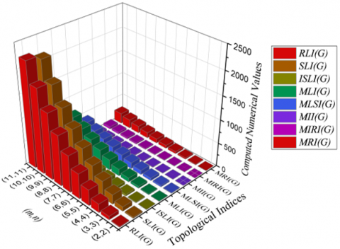
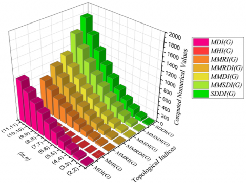
Table 6. Calculated bond additive numerical value
|
$\left( m,n \right)$ |
$RLI\left( G \right)$ |
$SLI\left( G \right)$ |
$ISLI\left( G \right)$ |
$MLI\left( G \right)$ |
$MLSI\left( G \right)$ |
$MII\left( G \right)$ |
$MIRI\left( G \right)$ |
$MRI\left( G \right)$ |
|
(2,2) |
15 |
25 |
6 |
6 |
11 |
2 |
2 |
5 |
|
(3,3) |
78 |
94 |
17 |
17 |
31 |
4 |
4 |
15 |
|
(4,4) |
186 |
204 |
35 |
44 |
57 |
7 |
7 |
29 |
|
(5,5) |
340 |
355 |
59 |
87 |
90 |
11 |
11 |
47 |
|
(6,6) |
540 |
548 |
89 |
147 |
130 |
15 |
16 |
68 |
|
(7,7) |
784 |
782 |
125 |
222 |
175 |
20 |
21 |
93 |
|
(8,8) |
1075 |
1058 |
167 |
313 |
228 |
26 |
27 |
121 |
|
(9,9) |
1411 |
1376 |
216 |
420 |
286 |
32 |
34 |
153 |
|
(10,10) |
1793 |
1735 |
271 |
544 |
352 |
39 |
41 |
189 |
|
(11,11) |
2220 |
2135 |
332 |
683 |
424 |
47 |
50 |
228 |
|
$\left( m,n \right)$ |
$MDI\left( G \right)$ |
$MHI\left( G \right)$ |
$MMRI\left( G \right)$ |
$MMRDI\left( G \right)$ |
$MMDI\left( G \right)$ |
$MMSDI\left( G \right)$ |
$SDDI\left( G \right)$ |
|
|
(2,2) |
16 |
2 |
10 |
15 |
20 |
18 |
28 |
|
|
(3,3) |
60 |
3 |
33 |
49 |
61 |
79 |
89 |
|
|
(4,4) |
120 |
5 |
71 |
100 |
121 |
167 |
183 |
|
|
(5,5) |
196 |
7 |
124 |
169 |
202 |
280 |
310 |
|
|
(6,6) |
288 |
10 |
191 |
256 |
303 |
419 |
471 |
|
|
(7,7) |
396 |
13 |
273 |
361 |
423 |
584 |
665 |
|
|
(8,8) |
520 |
16 |
369 |
484 |
564 |
776 |
892 |
|
|
(9,9) |
660 |
20 |
480 |
624 |
725 |
993 |
1153 |
|
|
(10,10) |
816 |
24 |
605 |
782 |
905 |
1236 |
1447 |
|
|
(11,11) |
988 |
29 |
745 |
958 |
1106 |
1505 |
1774 |
|
The numerical values are presented in Table 6 and graphical representations of various bond-additive molecular descriptors for Mesh Derived Network $MD{{N}_{1}}\left( m,n \right)$ structures are presented in Figure 7.
Let $G$ be the $MD{{N}_{2}}\left( m,n \right)$ network with defining parameters as $m$ and $n$. The number of vertices and edges in $MD{{N}_{2}}\left( m,n \right)$ are $2mn-m-n+1$ and $8\left( mn-m-n+1 \right)$ respectively. The edge partition and the end vertex degree sum is given in the Table 7.
Table 7. Mesh derived network $MD{{N}_{2}}\left( m,n \right)$
|
$\left( {{d}_{u}},{{d}_{v}} \right)$ |
No. of Edges |
|
(3,5) |
8 |
|
(3,6) |
4 |
|
(5,5) |
$2\left( m+n-6 \right)$ |
|
(5,6) |
8 |
|
(5,7) |
$4\left( m+n-6 \right)$ |
|
(5,8) |
$2\left( m+n-4 \right)$ |
|
(6,7) |
8 |
|
(6,8) |
4 |
|
(7,7) |
$2\left( m+n-8 \right)$ |
|
(7,8) |
$6\left( m+n-6 \right)$ |
|
(8,8) |
$(8mn-24\left( m+n \right)+72$) |
|
Theorem 4. Let G be a mesh derived network $MD{{N}_{2}}\left( m,n \right)$, then |
|
1. $RLI\left( G \right)=34.5912mn-47.5224m-47.5224n+59.9386$. 2. $SLI\left( G \right)=23.072mn-25.464m-25.464n+26.7476$. 3. $ISLI\left( G \right)=2.7739mn-2.4623m-2.4623n+2.4124$. 4. $MLI\left( G \right)=3.087m+3.087n-5.9404$. 5. $MLSI\left( G \right)=11.4778m+11.4778n-20.1084$. 6. $MII\left( G \right)=\left( 17m+17n-9 \right)/35$. 7. $MIRI\left( G \right)=0.6107m+0.6107n-0.79950$. 8. $MRI\left( G \right)=3.9190m+3.9190n-9.4500$. 9. $MDI\left( G \right)=20m+20n-56$. 10. $MHI\left( G \right)=\left( 11m+11n+32 \right)/64$. 11. $MMRI\left( G \right)=8mn-9.4256m-9.4256n+10.9148$. 12. $MMRDI\left( G \right)=8mn-6.3232m-6.3232n+5.0068$. 13. $MMDI\left( G \right)=\left( 280mn-152m-152n+72 \right)/35$. 14. $MMSDI\left( G \right)=(8820mn+8784m+8784n-3085)/11025$. 15. $SDDI\left( G \right)=\left( 3360mn-3147m-3147n+3305 \right)/210$. |
Proof.
In this theorem, we derive all 15 indices for $M D N_2$ using the vertex degree pairs $(3,5),(3,6),(5,5),(5,6),(5,7),(5,8)$, $(6,7),(6,8),(7,7),(7,8)$, and $(8,8)$ with corresponding edge counts $8,4,2(m+n-6), 8,4(m+n-6), 2(m+n-4)$, $8,4,2(m+n-8), 6(m+n-6)$, and $(8 m n-24(m+ n)+72$). These edge-vertex characteristics form the foundation for obtaining exact results for each index.
$\begin{aligned} R L I(G)& =\sum_{u v \in E(G)} ln d_G(u) ln d_G(v) =(ln 3 \times ln 5)(8)+(ln 3 \times ln 6)(4)+(ln 5 \times ln 5)(2(m+n-6))\\ & +(ln 5 \times ln 6)(8)+(ln 5 \times ln 7)(4(m+n-6))+(ln 5 \times ln 8)(2(m+n-4))+ (ln 6 \times ln 7)(8))\\ & +(ln 6 \times ln 8)(4))+(ln 7 \times ln 7)(2(m+n-8))+(ln 7 \times ln 8)(6(m+n-6))\\ & + (ln 8 \times ln 8)(8 m n-24(m+n)+72) =34.5912 m n-47.5224 m-47.5224 n+59.9386\end{aligned}$
$\begin{aligned} {SLI}(G)& =\sum_{u v \in E(G)} \sqrt{ln \left(d_u\right)}+\sqrt{ln \left(d_v\right)} =[\sqrt{ln (3)}+\sqrt{\ln (5)}](8)+[\sqrt{ln (3)}+\sqrt{ln (6)}](4)\\ &+ {[\sqrt{ln (5)}+\sqrt{ln (5)}](2(m+n-6))+[\sqrt{ln (5)}+} \sqrt{ln (6)}](8)+[\sqrt{ln (5)}+\sqrt{ln (7)}](4(m+n-6))\\ &+ {[\sqrt{ln (5)}+\sqrt{ln (8)}](2(m+n-4))+[\sqrt{ln (6)}+} \sqrt{\ln (7)}](8)+[\sqrt{ln (6)}+\sqrt{ln (8)}](4)+[\sqrt{\ln (7)}\\ &+ \sqrt{ln (7)}](2(m+n-8))+[\sqrt{ln (7)}+\sqrt{ln (8)}](6(m+ n-6))+[\sqrt{ln (8)}+\sqrt{ln (8)}](8 m n-24(m+n)+72) \\ &=23.072 m n-25.464 m-25.464 n+26.7476\end{aligned}$
$\begin{aligned}& {ISLI}(G)=\sum_{u v \in E(G)} \frac{1}{\sqrt{\ln \left(d_u\right)}+\sqrt{\ln \left(d_v\right)}} =\left[\frac{1}{\sqrt{\ln (3)}+\sqrt{\ln (5)}}\right](8)+\left[\frac{1}{\sqrt{\ln (3)}+\sqrt{\ln (6)}}\right](4)+ \\
& {\left[\frac{1}{\sqrt{\ln (5)}+\sqrt{\ln (5)}}\right](2(m+n-6))+\left[\frac{1}{\sqrt{\ln (5)}+\sqrt{\ln (6)}}\right](8)+} {\left[\frac{1}{\sqrt{\ln (5)}+\sqrt{\ln (7)}}\right](4(m+n-6))+} \\
& {\left[\frac{1}{\sqrt{\ln (5)}+\sqrt{\ln (8)}}\right](2(m+n-4))+\left[\frac{1}{\sqrt{\ln (6)}+\sqrt{\ln (7)}}\right](8)+} {\left[\frac{1}{\sqrt{\ln (6)}+\sqrt{\ln (8)}}\right](4)+\left[\frac{1}{\sqrt{\ln (7)}+\sqrt{\ln (7)}}\right](2(m+n-8))+} \\
& {\left[\frac{1}{\sqrt{\ln (7)}+\sqrt{\ln (8)}}\right](6(m+n-6))+} {\left[\frac{1}{\sqrt{\ln (8)}+\sqrt{\ln (8)}}\right](8 m n-24(m+n)+72)} \\
& =2.7739 m n-2.4623 m-2.4623 n+2.4124\end{aligned}$
$\begin{aligned} & M L I(G)=\sum_{u v \in E(G)}\left|\ln d_u-\ln d_v\right| \\ & =|\ln 3-\ln 5|(8)+|\ln 3-\ln 6|(4)+\mid \ln 5- \\ & \ln 5|(2(m+n-6))+|\ln 5-\ln 6|(8)+| \ln 5- \\ & \ln 7|(4(m+n-6))+|\ln 5-\ln 8|(2(m+n-4))+ \\ & |\ln 6-\ln 7|(8)+|\ln 6-\ln 8|(4)+|\ln 7-\ln 7|(2(m+ n-8))+\\ &|\ln 7-\ln 8|(6(m+n-6))+\mid \ln 8- \ln 8 \mid(8 m n-24(m+n)+72) \\ & =3.087 m+3.087 n-5.9404\end{aligned}$
$\begin{aligned} & {MLSI}(G)=\sum_{u v \in E(G)}\left|\ln ^2 d_u-\ln ^2 d_v\right| \\ & =\left|\ln ^2 3-\ln ^2 5\right|(8)+\left|\ln ^2 3-\ln ^2 6\right|(4)+\mid \ln ^2 5- \\ & \ln ^2 5\left|(2(m+n-6))+\left|\ln ^2 5-\ln ^2 6\right|(8)+\right| \ln ^2 5- \\ & \ln ^2 7\left|(4(m+n-6))+\left|\ln ^2 5-\ln ^2 8\right|(2(m+n-\right. \\ & 4))+\left|\ln ^2 6-\ln ^2 7\right|(8)+\left|\ln ^2 6-\ln ^2 8\right|(4)+\mid \ln ^2 7- \\ & \ln ^2 7\left|(2(m+n-8))+\left|\ln ^2 7-\ln ^2 8\right|(6(m+n-\right. \\ & 6))+\left|\ln ^2 8-\ln ^2 8\right|(8 m n-24(m+n)+72) \\ & =11.4778 m+11.4778 n-20.1084\end{aligned}$
$\begin{aligned} &{MII}(G)=\sum_{u v \in E(G)}\left|\frac{1}{d_u}-\frac{1}{d_v}\right| =\left|\frac{1}{3}-\frac{1}{5}\right|(8)+\left|\frac{1}{3}-\frac{1}{6}\right|(4)\\ &+\left|\frac{1}{5}-\frac{1}{5}\right|(2(m+n-6))+ \left|\frac{1}{5}-\frac{1}{6}\right|(8)+\left|\frac{1}{5}-\frac{1}{7}\right|(4(m+n-6)) \\ &+\left|\frac{1}{5}-\frac{1}{8}\right|(2(m+ n-4))+\left|\frac{1}{6}-\frac{1}{7}\right|(8)+\left|\frac{1}{6}-\frac{1}{8}\right|(4)+\left|\frac{1}{7}-\frac{1}{7}\right|(2(m+ n-8))\\ &+\left|\frac{1}{7}-\frac{1}{8}\right|(6(m+n-6))+\left|\frac{1}{8}-\frac{1}{8}\right|(8 m n- 24(m+n)+72) \\ & =(17 m+17 n-9) / 35\end{aligned}$
$\begin{aligned} &{MIRI}(G)=\sum_{u v \in E(G)}\left|\frac{1}{\sqrt{d_u}}-\frac{1}{\sqrt{d_v}}\right| =\left|\frac{1}{\sqrt{3}}-\frac{1}{\sqrt{5}}\right|(8)+\left|\frac{1}{\sqrt{3}}-\frac{1}{\sqrt{6}}\right|(4)\\ &+\left|\frac{1}{\sqrt{5}}-\frac{1}{\sqrt{5}}\right|(2(m+n- 6))+\left|\frac{1}{\sqrt{5}}-\frac{1}{\sqrt{6}}\right|(8)+\left|\frac{1}{\sqrt{5}}-\frac{1}{\sqrt{7}}\right|(4(m+n-6))\\ &+ \left|\frac{1}{\sqrt{5}}-\frac{1}{\sqrt{8}}\right|(2(m+n-4))+\left|\frac{1}{\sqrt{6}}-\frac{1}{\sqrt{7}}\right|(8)+\left\lvert\, \frac{1}{\sqrt{6}}-\right. \\ &\frac{1}{\sqrt{8}}\left|(4) +\left|\frac{1}{\sqrt{7}}-\frac{1}{\sqrt{7}}\right|(2(m+n-8))+\left|\frac{1}{\sqrt{7}}-\frac{1}{\sqrt{8}}\right|(6(m+\right. n-6))\\ &+\left|\frac{1}{\sqrt{8}}-\frac{1}{\sqrt{8}}\right|(8 m n-24(m+n)+72) \\ & =0.6107 m+0.6107 n-0.79950\end{aligned}$
$\begin{aligned} & {MRI}(G)=\sum_{u v \in E(G)}\left|\sqrt{d_u}-\sqrt{d_v}\right| =|\sqrt{3}-\sqrt{5}|(8)+|\sqrt{3}-\sqrt{6}|(4)\\ &+|\sqrt{5}-\sqrt{5}|(2(m+n- 6))+|\sqrt{5}-\sqrt{6}|(8)+|\sqrt{5}-\sqrt{7}|(4(m+n-6))\\ &+\mid \sqrt{5}- \sqrt{8}|(2(m+n-4))+|\sqrt{6}-\sqrt{7}|(8)+|\sqrt{6}-\sqrt{8}|(4)\\ &+ |\sqrt{7}-\sqrt{7}|(2(m+n-8))+|\sqrt{7}-\sqrt{8}|(6(m+n-6))\\ &+ |\sqrt{8}-\sqrt{8}|(8 m n-24(m+n)+72))=3.9190 m+ 3.9190 n-9.4500\end{aligned}$
$\begin{aligned} & {MDI}(G)=\sum_{u v \in E(G)}\left|d_u-d_v\right| =|3-5|(8)+|3-6|(4)+|5-5|(2(m+n-6))\\ &+\mid 5- 6|(8)+|5-7|(4(m+n-6))+|5-8|(2(m+n-4))\\ &+ |6-7|(8)+|6-8|(4)+|7-7|(2(m+n-8))\\ &+ |7-8|(6(m+n-6))+|8-8|(8 m n-24(m+n)+72)\\ &= 20 m+20 n-56\end{aligned}$
$\begin{aligned} & {MHI}(G)=\sum_{u v \in E(G)}\left|\left(\frac{1}{2}\right)^{d_u}-\left(\frac{1}{2}\right)^{d_v}\right| =\left|\left(\frac{1}{2}\right)^3-\left(\frac{1}{2}\right)^5\right|((8))+\left|\left(\frac{1}{2}\right)^3-\left(\frac{1}{2}\right)^6\right|(4)\\ &+\left\lvert\,\left(\frac{1}{2}\right)^5-\right. \left(\frac{1}{2}\right)^5\left|(2(m+n-6))+\left|\left(\frac{1}{2}\right)^5-\left(\frac{1}{2}\right)^6\right|(8)+\right|\left(\frac{1}{2}\right)^5\\ &- \left(\frac{1}{2}\right)^7\left|(4(m+n-6))+\left|\left(\frac{1}{2}\right)^5-\left(\frac{1}{2}\right)^8\right|(2(m+n-4))+\right. \\ & \left|\left(\frac{1}{2}\right)^6-\left(\frac{1}{2}\right)^7\right|(8)+\left|\left(\frac{1}{2}\right)^6-\left(\frac{1}{2}\right)^8\right|(4)+\left|\left(\frac{1}{2}\right)^7-\left(\frac{1}{2}\right)^7\right|(2(m+ n-8))\\ &+\left|\left(\frac{1}{2}\right)^7-\left(\frac{1}{2}\right)^8\right|(6(m+n-6))+\left\lvert\,\left(\frac{1}{2}\right)^8-\right. \left.\left(\frac{1}{2}\right)^8 \right\rvert\,(8 m n-24(m+n)+72) \\ & =(11 m+11 n+32) / 64\end{aligned}$
$\begin{aligned} & {MMRI}(G)=\sum_{u v \in E(G)} \sqrt{\frac{\operatorname{mini}\left(d_u, d_v\right)}{\operatorname{maxi}\left(d_u, d_v\right)}} =\sqrt{\frac{\operatorname{mini}(3,5)}{\operatorname{maxi}(3,5)}}(8)+\sqrt{\frac{\operatorname{mini}(3,6)}{\operatorname{maxi}(3,6)}}(4)\\ &+\sqrt{\frac{\operatorname{mini}(5,5)}{\operatorname{maxi}(5,5)}}(2(m+n- 6))+\sqrt{\frac{\operatorname{mini}(5,6)}{\max i(5,6)}}(8)+\sqrt{\frac{\operatorname{mini}(5,7)}{\operatorname{maxi}(5,7)}}(4(m+n-6))\\ &+ \sqrt{\frac{\operatorname{mini}(5,8)}{\operatorname{maxi}(5,8)}}(2(m+n-4))+\sqrt{\frac{\operatorname{mini}(6,7)}{\operatorname{maxi}(6,7)}}(8)\\ &+ \sqrt{\frac{\operatorname{mini}(6,8)}{\operatorname{maxi}(6,8)}}(4)+\sqrt{\frac{\operatorname{mini}(7,7)}{\operatorname{maxi}(7,7)}}(2(m+n-8)) \\ &+ \sqrt{\frac{\operatorname{mini}(7,8)}{\operatorname{maxi}(7,8)}}(6(m+n-6))+\sqrt{\frac{\operatorname{mini}(8,8)}{\operatorname{maxi}(8,8)}}(8 m n-24(m+ n)+72))\\ &=8 m n-9.4256 m-9.4256 n+10.9148\end{aligned}$
$\begin{aligned} & {MMRDI}(G)=\sum_{u v \in E(G)} \sqrt{\frac{\operatorname{maxi}\left(d_u, d_v\right)}{\operatorname{mini}\left(d_u, d_v\right)}} =\sqrt{\frac{\operatorname{maxi}(3,5)}{\operatorname{mini}(3,5)}}(8)+\sqrt{\frac{\operatorname{maxi}(3,6)}{\operatorname{mini}(3,6)}}(4)\\ &+\sqrt{\frac{\operatorname{maxi}(5,5)}{\operatorname{mini}(5,5)}}(2(m+ n-6))+\sqrt{\frac{\operatorname{maxi}(5,6)}{\operatorname{mini}(5,6)}}(8)+\sqrt{\frac{\operatorname{maxi}(5,7)}{\operatorname{mini}(5,7)}}(4(m+n-6)) \\ &+ \sqrt{\frac{\operatorname{maxi}(5,8)}{\operatorname{mini}(5,8)}}(2(m+n-4))+\sqrt{\frac{\operatorname{maxi}(6,7)}{\operatorname{mini}(6,7)}}(8)+ \sqrt{\frac{\operatorname{maxi}(6,8)}{\operatorname{mini}(6,8)}}(4)\\ &+\sqrt{\frac{\operatorname{maxi}(7,7)}{\operatorname{mini}(7,7)}}(2(m+n-8))+ \sqrt{\frac{\operatorname{maxi}(7,8)}{\min i(7,8)}}(6(m+n-6))\\ &+\sqrt{\frac{\operatorname{maxi}(8,8)}{\operatorname{mini}(8,8)}}(8 m n-24(m+ n)+72))=8 m n-6.3232 m-6.3232 n+5.0068\end{aligned}$
$\begin{aligned} & M M D I(G)=\sum_{u v \in E(G)} \frac{\max \left(d_u, d_v\right)}{\min \left(d_u, d_v\right)} =\frac{\max (3,5)}{\min (3,5)}(8)+\frac{\max (3,6)}{\min (3,6)}(4)\\ &+\frac{\max (5,5)}{\min (5,5)}(2(m+n-6))+ \frac{\max (5,6)}{\min (5,6)}(8)+\frac{\max (5,7)}{\min (5,7)}(4(m+n-6))\\ &+\frac{\operatorname{maxi}(5,8)}{\operatorname{mini}(5,8)}(2(m+n- 4))+\frac{\operatorname{maxi}(6,7)}{\min (6,7)}(8)+\frac{\operatorname{maxi}(6,8)}{\operatorname{mini}(6,8)}(4)+\frac{\operatorname{maxi}(7,7)}{\operatorname{mini}(7,7)}(2(m+n-8))\\ &+ \left.\frac{\operatorname{maxi}(7,8)}{\operatorname{mini}(7,8)}(6(m+n-6))+\frac{\operatorname{maxi}(8,8)}{\operatorname{mini}(8,8)}(8 m n-24(m+n)+72)\right) \\ & =(280 m n-152 m-152 n+72) / 35\end{aligned}$
$\begin{aligned} & {MMSDI}(G)=\sum_{u v \in E(G)}\left(\frac{\operatorname{maxi}\left(d_u, d_v\right)}{\operatorname{mini}\left(d_u, d_v\right)}\right)^2 =\left(\frac{\operatorname{maxi}(3,5)}{\operatorname{mini}(3,5)}\right)^2(8)+\left(\frac{\operatorname{maxi}(3,6)}{\operatorname{mini}(3,6)}\right)^2(4)\\ &+\left(\frac{\operatorname{maxi}(5,5)}{\operatorname{mini}(5,5)}\right)^2(2(m+n- 6))+\left(\frac{\operatorname{maxi}(5,6)}{\operatorname{mini}(5,6)}\right)^2(8)+\left(\frac{\operatorname{maxi}(5,7)}{\operatorname{mini}(5,7)}\right)^2(4(m+n-6))\\ &+ \left(\frac{\operatorname{maxi}(5,8)}{\operatorname{mini}(5,8)}\right)^2(2(m+n-4))+\left(\frac{\operatorname{maxi}(6,7)}{\operatorname{mini}(6,7)}\right)^2(8)+ \left(\frac{\operatorname{maxi}(6,8)}{\operatorname{mini}(6,8)}\right)^2(4)\\ &+\left(\frac{\operatorname{maxi}(7,7)}{\operatorname{mini}(7,7)}\right)^2(2(m+n-8))+ \left(\frac{\operatorname{maxi}(7,8)}{\operatorname{mini}(7,8)}\right)^2(6(m+n-6))\\ &+\left(\frac{\operatorname{maxi}(8,8)}{\operatorname{mini}(8,8)}\right)^2(8 m n-24(m+ n)+72))=(8820 m n+8784 m+8784 n-3085) / 11025\end{aligned}$
$\begin{aligned} & {SDDI}(G)=\sum_{u v \in E(G)}\left[\frac{\operatorname{mini}\left(d_u, d_v\right)}{\operatorname{maxi}\left(d_u, d_v\right)}+\frac{\operatorname{maxi}\left(d_u, d_v\right)}{\operatorname{mini}\left(d_u, d_v\right)}\right] =\left[\frac{\operatorname{mini}(3,5)}{\operatorname{maxi}(3,5)}+\frac{\operatorname{maxi}(3,5)}{\operatorname{mini}(3,5)}\right](8) \\ &+\left[\frac{\operatorname{mini}(3,6)}{\operatorname{maxi}(3,6)}+\frac{\operatorname{maxi}(3,6)}{\operatorname{mini}(3,6)}\right](4)+ {\left[\frac{\operatorname{mini}(5,5)}{\operatorname{maxi}(5,5)}+\frac{\operatorname{maxi}(5,5)}{\operatorname{mini}(5,5)}\right](2(m+n-6))+\left[\frac{\operatorname{mini}(5,6)}{\operatorname{maxi}(5,6)}+\right.} \\ & \left.\frac{\operatorname{maxi}(5,6)}{\operatorname{mini}(5,6)}\right](8)+\left[\frac{\operatorname{mini}(5,7)}{\operatorname{maxi}(5,7)}+\frac{\operatorname{maxi}(5,7)}{\operatorname{mini}(5,7)}\right](4(m+n-6))\\ &+ {\left[\frac{\operatorname{mini}(5,8)}{\operatorname{maxi}(5,8)}+\frac{\operatorname{maxi}(5,8)}{\operatorname{mini}(5,8)}\right](2(m+n-4))+\left[\frac{\operatorname{mini}(6,7)}{\operatorname{maxi}(6,7)}+\right.} \left.\frac{\operatorname{maxi}(6,7)}{\operatorname{mini}(6,7)}\right](8)\\ &+\left[\frac{\operatorname{mini}(6,8)}{\operatorname{maxi}(6,8)}+\frac{\operatorname{maxi}(6,8)}{\operatorname{mini}(6,8)}\right](4)+\left[\frac{\operatorname{mini}(7,7)}{\operatorname{maxi}(7,7)}+\right. \left.\frac{\operatorname{maxi}(7,7)}{\operatorname{mini}(7,7)}\right](2(m+n-8))\\ &+\left[\frac{\operatorname{mini}(7,8)}{\operatorname{maxi}(7,8)}+\frac{\operatorname{maxi}(7,8)}{\operatorname{mini}(7,8)}\right](6(m+ n-6))\\ &+\left[\frac{\operatorname{mini}(8,8)}{\operatorname{maxi}(8,8)}+\frac{\operatorname{maxi}(8,8)}{\operatorname{mini}(8,8)}\right](8 m n-24(m+n)+ 72)\\ &=(3360 \operatorname{mn}-3147 m-3147 n+3305) / 210\end{aligned}$
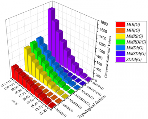
The numerical values are presented in Table 8 and graphical representations of various bond-additive molecular descriptors for mesh derived network ${MDN}_2(m, n)$ structures are presented in Figure 8.
Table 8. Calculated bond additive numerical value
|
$\left( m,n \right)$ |
$RLI\left( G \right)$ |
$SLI\left( G \right)$ |
$ISLI\left( G \right)$ |
$MLI\left( G \right)$ |
$MLSI\left( G \right)$ |
$MII\left( G \right)$ |
$MIRI\left( G \right)$ |
$MRI\left( G \right)$ |
|
(2,2) |
8 |
17 |
4 |
6 |
26 |
2 |
2 |
6 |
|
(3,3) |
86 |
82 |
13 |
13 |
49 |
3 |
3 |
14 |
|
(4,4) |
233 |
192 |
27 |
19 |
72 |
4 |
4 |
22 |
|
(5,5) |
449 |
349 |
47 |
25 |
95 |
5 |
5 |
30 |
|
(6,6) |
735 |
552 |
73 |
31 |
118 |
6 |
7 |
38 |
|
(7,7) |
1090 |
801 |
104 |
37 |
141 |
7 |
8 |
45 |
|
(8,8) |
1513 |
1096 |
141 |
43 |
164 |
8 |
9 |
53 |
|
(9,9) |
2006 |
1437 |
183 |
50 |
186 |
8 |
10 |
61 |
|
(10,10) |
2569 |
1825 |
231 |
56 |
209 |
9 |
11 |
69 |
|
(11,11) |
3200 |
2258 |
284 |
62 |
232 |
10 |
13 |
77 |
|
$\left( m,n \right)$ |
$MDI\left( G \right)$ |
$MHI\left( G \right)$ |
$MMRI\left( G \right)$ |
$MMRDI\left( G \right)$ |
$MMDI\left( G \right)$ |
$MMSDI\left( G \right)$ |
$SDDI\left( G \right)$ |
|
|
(2,2) |
24 |
1 |
5 |
12 |
17 |
6 |
20 |
|
|
(3,3) |
64 |
2 |
26 |
39 |
48 |
12 |
70 |
|
|
(4,4) |
104 |
2 |
64 |
82 |
95 |
19 |
152 |
|
|
(5,5) |
144 |
2 |
117 |
142 |
159 |
28 |
266 |
|
|
(6,6) |
184 |
3 |
186 |
217 |
238 |
38 |
412 |
|
|
(7,7) |
224 |
3 |
271 |
308 |
333 |
50 |
590 |
|
|
(8,8) |
264 |
3 |
372 |
416 |
445 |
64 |
800 |
|
|
(9,9) |
304 |
4 |
489 |
539 |
572 |
79 |
1042 |
|
|
(10,10) |
344 |
4 |
622 |
679 |
715 |
96 |
1316 |
|
|
(11,11) |
384 |
4 |
772 |
834 |
875 |
114 |
1622 |
|
(a)
(b)
Figure 8. A visual representation of molecular characteristics for bond addition of mesh derived network $MD{{N}_{2}}\left( m,n \right)$
Using the Adriatic index suite as bond-additive molecular descriptors, this study provides a methodical, degree-based examination of butterfly, benes and $M D N_1$ and $M D N_2$. For each type of network, the study calculates numerical values and derives closed-form formulas to quantify important structural qualities like fault tolerance, regularity, connectedness, and redundancy. Key insights can be obtained by comparing the tabular statistics and graphical trends: Despite their high regularity and predictable low-latency connectivity, Butterfly Networks are not flexible or fault-tolerant. Benes Networks get around these restrictions by using symmetric, rearranging designs that improve robustness, scalability, and routing possibilities. The highest robustness and adaptability are offered by $M D N_1$ and $M D N_2$, whose higher imbalance and ratio-based Adriatic index values represent their superior connectivity, balance, and fault tolerance due to their unique architecture and additional linkages.
[1] B Beneš, V.E. (Ed.). (1965). Mathematics in Science and Engineering Vol. 17: Mathematical Theory of Connecting Networks and Telephone Traffic. Academic Press.
[2] Imran, M., Hayat, S., Mailk, M.Y.H. (2014). On topological indices of certain interconnection networks. Applied Mathematics and Computation, 244: 936-951. https://doi.org/10.1016/j.amc.2014.07.064
[3] Xu, J. (2013). Topological Structure and Analysis of Interconnection Networks. Springer New York, NY. https://doi.org/10.1007/978-1-4757-3387-7
[4] Manuel, P.D., Abd-El-Barr, M.I., Rajasingh, I., Rajan, B. (2008). An efficient representation of Benes networks and its applications. Journal of Discrete Algorithms, 6(1): 11-19. https://doi.org/10.1016/j.jda.2006.08.003
[5] Konstantinidou, S. (1993). The selective extra stage butterfly. IEEE Transactions on Very Large Scale Integration (VLSI) Systems, 1(2): 167-171. http://doi.org/10.1109/92.238419
[6] Liu, X.C., Gu, Q.P. (2002). Multicasts on WDM all-optical butterfly networks. Journal of Information Science and Engineering, 18(6): 1049-1058. http://doi.org/10.6688/JISE.2002.18.6.5
[7] Chen, M.S., Shin, K.G., Kandlur, D.D. (1990). Addressing, routing, and broadcasting in hexagonal mesh multiprocessors. IEEE Transactions on Computers, 39(1): 10-18. https://doi.org/10.1109/12.46277
[8] Cynthia, V.J.A. (2014). Metric dimension of certain mesh derived graphs. Journal of Computer and Mathematical Sciences, 5(1): 1-122.
[9] Jiang, L.L., Perc, M. (2013). Spreading of cooperative behaviour across interdependent groups. Scientific Reports, 3(1): 2483. https://doi.org/10.1038/srep02483
[10] Perc, M., Grigolini, P. (2013). Collective behavior and evolutionary games an introduction, Chaos Soliton Fract, 6: 20-27. https://doi.org/10.1016/j.chaos.2013.06.002
[11] Perc, M., Gómez-Gardenes, J., Szolnoki, A., Floría, L. M., Moreno, Y. (2013). Evolutionary dynamics of group interactions on structured populations: A review. Journal of the Royal Society Interface, 10(80): 20120997. https://doi.org/10.1098/rsif.2012.0997
[12] Perc, M., Szolnoki, A. (2010). Coevolutionary games—A mini review. BioSystems, 99(2): 109-125. https://doi.org/10.1016/j.biosystems.2009.10.003
[13] Wang, Z., Szolnoki, A., Perc, M. (2012). Evolution of public cooperation on interdependent networks: The impact of biased utility functions. Europhysics Letters, 97(4): 48001. https://doi.org/10.1209/0295-5075/97/48001
[14] Wang, Z., Szolnoki, A., Perc, M. (2013). Interdependent network reciprocity in evolutionary games. Scientific Reports, 3(1): 1183. https://doi.org/10.1038/srep01183
[15] Wang, Z., Szolnoki, A., Perc, M. (2014). Self-organization towards optimally interdependent networks by means of coevolution. New Journal of Physics, 16(3): 033041. https://doi.org/10.1088/1367-2630/16/3/033041
[16] Yang, Y.M., Qiu, W.Y. (2007). Molecular design and mathematical analysis of carbon cylinder links, MATCH Communications in Mathematical and in Computer Chemistry, 58: 435-447.
[17] Trinajstic, N. (2018). Chemical Graph Theory. CRC Press. https://doi.org/10.1201/9781315139111
[18] Todeschini, R., Consonni, V. (2008). Handbook of Molecular Descriptors. John Wiley & Sons. https://doi.org/10.1002/9783527613106
[19] Yousefi-Azari, H., Khalifeh, M.H., Ashrafi, A.R. (2011). Calculating the edge Wiener and edge Szeged indices of graphs. Journal of Computational and Applied Mathematics, 235(16): 4866-4870. https://doi.org/10.1016/j.cam.2011.02.019
[20] Vukičević, D., Gašperov, M. (2010). Bond additive modeling 1. Adriatic indices. Croatica Chemica Acta, 83(3): 243-260.
[21] Prabhu, S., Murugan, G., Sudhakhar, K.S. (2018). On the new topological index of certain nanostructures using combinatorial computation. Journal of Mathematics and Computer Science, 9(9): 1257-1265. http://doi.org/10.29055/jcms/865
[22] Prabhu, S., Murugan, G., Muthuraman, N. (2018). On degree-distance index of hexagonal network. International Journal of Advanced Research in Basic Engineering Sciences and Technology, 4(3): 24-33.
[23] Prabhu, S., Murugan, G., Cary, M., Arulperumjothi, M., Liu, J.B. (2020). On certain distance and degree based topological indices of Zeolite LTA frameworks. Materials Research Express, 7(5): 055006. https://doi.org/10.1088/2053-1591/ab8b18
[24] Prabhu, S., Murugan, G., Arockiaraj, M., Arulperumjothi, M., Manimozhi, V. (2021). Molecular topological characterization of three classes of polycyclic aromatic hydrocarbons. Journal of Molecular Structure, 1229: 129501. https://doi.org/10.1016/j.molstruc.2020.129501
[25] Prabhu, S., Murugan, G., Therese, S.K., Arulperumjothi, M., Siddiqui, M.K. (2022). Molecular structural characterization of cycloparaphenylene and its variants. Polycyclic Aromatic Compounds, 42(8): 5550-5566. https://doi.org/10.1080/10406638.2021.1942082
[26] Prabhu, S., Arulperumjothi, M., Murugan, G., Dhinesh, V.M., Kumar, J.P. (2019). On certain counting polynomial of titanium dioxide nanotubes. Nanoscience & Nanotechnology-Asia, 9(2): 240-243. https://doi.org/10.2174/2210681208666180322120144
[27] Prabhu, S., Murugan, G., Arulperumjothi, M. (2021). On the edge-version of topological indices of titanium dioxide nanotube and nanosheet. Nanoscience & Nanotechnology-Asia, 11(2): 174-188. https://doi.org/10.2174/2210681210999200423120222
[28] Murugan, G., Julietraja, K., Alsinai, A. (2023). Computation of neighborhood M-polynomial of cycloparaphenylene and its variants. ACS Omega, 8(51): 49165-49174. https://doi.org/10.1021/acsomega.3c07294
[29] Tharmalingam, G., Ponnusamy, K., Govindhan, M., Konsalraj, J. (2023). On certain degree based and bond additive molecular descriptors of hexabenzocorenene. Biointerface Research in Applied Chemistry, 13(5): 495. https://doi.org/10.33263/briac135.495
[30] Gunasekar, T., Kathavarayan, P., Alsinai, A., Murugan, G. (2024). On certain degree based and bond-additive topological indices of dodeca-benzo-circumcorenene. Combinatorial Chemistry & High Throughput Screening, 27(11): 1629-1641. https://doi.org/10.2174/0113862073274943231211110011
[31] Chu, Y.M., Julietraja, K., Venugopal, P., Siddiqui, M.K., Prabhu, S. (2021). Degree-and irregularity-based molecular descriptors for benzenoid systems. The European Physical Journal Plus, 136(1): 1-17. https://doi.org/10.1140/epjp/s13360-020-01033-z
[32] Julietraja, K., Venugopal, P., Prabhu, S., Liu, J.B. (2022). M-polynomial and degree-based molecular descriptors of certain classes of benzenoid systems. Polycyclic Aromatic Compounds, 42(6): 3450-3477. https://doi.org/10.1080/10406638.2020.1867205
[33] Yang, J., Konsalraj, J., Raja S, A.A. (2022). Neighbourhood sum degree-based indices and entropy measures for certain family of graphene molecules. Molecules, 28(1): 168. https://doi.org/10.3390/molecules28010168