Abdulmajeed Sulaiman*![]() | Farhad E. Mahmood
| Farhad E. Mahmood![]() | Sarah Kanaan Hamzah
| Sarah Kanaan Hamzah![]()
© 2025 The authors. This article is published by IIETA and is licensed under the CC BY 4.0 license (http://creativecommons.org/licenses/by/4.0/).
OPEN ACCESS
Accurate forecasting of global horizontal irradiance (GHI) is essential for optimizing solar power generation and ensuring reliable grid operation. Long-term predictions enhance grid planning and mitigate challenges arising from the inherent variability of solar radiation. This study addresses GHI forecasting for Mosul, Iraq, using the satellite-based MERRA-2 dataset and the XGBoost algorithm with tuned hyperparameters. The contributions are twofold: first, a systematic evaluation of rolling window sizes demonstrates that shorter windows substantially improve accuracy, with the best results achieved at a two-day window augmented by meteorological features, yielding an NRMSE of 0.0855, MAE of 546.6, and R2 of 0.907 compared to 0.83 NRMSE at a one-year window; second, a comparative benchmarking against LightGBM and LSTM establishes that XGBoost consistently outperforms these baselines, achieving lower error rates (LightGBM NRMSE = 0.251; LSTM NRMSE = 0.103) and greater stability across forecasting horizons. These findings highlight the decisive role of windowing strategies in boosting machine learning performance for solar irradiance forecasting and provide actionable insights for the design of more robust and efficient solar energy infrastructures.
long-term forecasting, LSTM, renewable energy, rolling window, solar irradiance, window size, XGBoost
In recent decades, Iraq has become fully dependent on oil and its derivatives. Although it relies heavily on oil, Iraq’s industrial and transportation sectors face significant challenges, so the Iraqi government is moving toward better power resources to cover the country's electricity needs; one of the most promising resources is solar energy. Iraq is in a very sunny area that has good solar irradiance every year [1]. In general, Iraq enjoys an average of 3,316 hours/year of solar radiation, of which 501 watts/m2 of solar energy incident on the Earth daily. In winter, Global Solar Radiation may decrease to 1.68 kW hr/m2, which is still high at this time of year. Mosul serves as a representative location for analyzing solar irradiance due to its substantial seasonal fluctuations. From very little irradiance during winter to fully sunny days in summer [2, 3]. In Iraq, as in other third-world countries, solar power measurements, transmission, and other infrastructure are very poor and difficult to obtain; incident solar radiation consists of a wide range of electromagnetic waves. Spectral wavelengths between 300–4000 nm are used to generate solar energy. The solar rays that fall within this range and reach Earth are divided into two parts: the reflected rays and the Global Horizontal Irradiance (GHI) we receive.
The relationship between extra-terrestrial radiation and global solar irradiance is represented by the term clarity index, indicated in Eq. (1), a high value of the clarity index indicates a sunny day and vice versa [4].
$K t=\frac{H}{H o}$ (1)
where, Kt represents the clearness index, horizontal radiation H, and Ho is the extraterrestrial radiation on a horizontal surface. Due to the variability of solar irradiance and according to the resolution factor and its variation throughout the year, month, week, and even day, historical records are used to build different statistical, physical, and machine learning models to obtain optimal power generation and grid construction [5-7].
The main contributions of this study are twofold:
(1). A systematic evaluation of rolling window sizes in the XGBoost framework for solar irradiance forecasting. By testing multiple window lengths, the study demonstrates how temporal context affects predictive accuracy, highlighting the trade-off between capturing long-term seasonal dynamics and short-term fluctuations.
(2). A comparative benchmarking against two widely used baseline models, LightGBM and LSTM, implemented under standard configurations with basic hyperparameter tuning. This design isolates the unique impact of the rolling window strategy in XGBoost and shows that the proposed approach achieves superior accuracy relative to methods that do not employ such a mechanism.
This paper is divided into six sections. In Section II, related works that involve different solar irradiance forecasting methods are discussed. In Section III, we introduce implemented methods in our work w. In Section IV, the implemented models and their results are explained. In Section V, the results are discussed further. Finally, in Section IV, the conclusions are discussed regarding future work.
2.1 Traditional methods
Nowadays, long-term solar irradiance forecasting is critical for power generation and grid construction. Numerous researchers have explored various approaches to achieve optimal system designs that provide more effective and quicker forecasting models. These models are crucial for constructing dependable and optimized solar power transportation networks along with other solar energy infrastructures. Multi-linear predictors are used on daily recorded data for the prediction of long-term GHI [8, 9].
2.2 Deep learning approaches
In recent discussions on artificial intelligence techniques for solar radiation estimation within renewable energy applications, several key methods have arisen that significantly enhance prediction accuracy and overall system efficiency [10]. One central approach is the use of Long Short-Term Memory (LSTM) networks, which have been effectively employed not only to forecast daily power generation but also to achieve reliable long-term seasonal predictions [11]. An important advancement involves the development of a hybrid model that combines Complete Ensemble Empirical Mode Decomposition with Adaptive Noise, Convolutional Neural Networks, and Long Short-Term Memory (CEEMDAN-CNN-LSTM). This innovative model is specifically designed for predicting hourly GHI and has been strictly evaluated using real-world datasets, showing promising results in terms of accuracy and applicability [12].
2.3 Hybrid deep learning models
Recent advancements in forecasting GHI have been significantly impacted by deep learning techniques, particularly when incorporating multi-site real data. Research suggests that prioritizing records from nearby weather stations can enhance the accuracy of these predictions [13]. A comprehensive review of existing deep learning models dedicated to GHI forecasting indicates a particular focus on hybrid architecture, especially those that combine CNN with LSTM networks. These hybrid models have shown considerable promise, improving the precision of forecasts by leveraging the strengths of both deep learning approaches [14]. The development of a hybrid CNN-LSTM approach has demonstrated the potential of integrating various deep learning techniques to yield more reliable GHI predictions, showcasing the continual evolution of forecasting methodologies in this field [15].
2.4 Gradient boosting models
To construct a strong forecasting system, various machine learning techniques are utilized, particularly Gradient Boosting Regression Trees (GBRT), XGBoost, random forests, and Gaussian Process Regression (GPR). These methods serve as different layers in a stacking ensemble, improving the overall predictive accuracy for both daily and monthly forecasts. Among these techniques, XGBoost has emerged as a particularly effective approach, renowned for its ability to deliver precise long-term predictions [16]. The XGBoost method is one of the new machine learning methods that produce more accurate results in long-term forecasting. The MERRA-2 database consists of 1490 days with solar irradiance taken daily. At the time of maximum daily irradiance, these 1490 records are divided into the training set and the test set [17].
2.5 Other advanced methods
Using a more modern method, LightGBM outclasses other machine learning and empirical models to forecast solar photovoltaic energy production [18]. A recent study employed Multi-Layer Perceptron Gated Recurrent Unit (GRU) combined with Principal Component Analysis (PCA) and grid search optimization for multi-horizon solar irradiance forecasting using multivariate datasets, demonstrating improved accuracy across different time scales due to effective feature reduction and hyperparameter tuning [19].
While previous studies have investigated various forecasting techniques, most did not systematically examine the effect of rolling window sizes on model accuracy, particularly when using gradient boosting approaches. This study addresses this gap by evaluating the impact of different rolling window sizes on XGBoost performance using the MERRA-2 dataset for Mosul, Iraq.
3.1 Performance analysis
Due to fluctuating power reaching the earth, any forecasting method will suffer from some errors, and the predicted data will not be very accurate. To decide if the implemented method was good or not, Root Means Square Error (RMSE), Normalized Root Means Square Error (NRMSE), Mean Absolute Error (MAE), and Coefficient of Determination (R2) are used to measure the deviation of forecast measurements due to their importance in time-series regression tasks:
$R M S E=\sqrt{\frac{1}{n}} * \sum\left(P_{ {pred }}-P_{{mean }}\right)^2$ (2)
where, $P_{pred}$ are the forecast values at each time, $P_{mean}$ are the measured values at each time, and in the number of sample data for the period, from Eq. (2), if RMSE is lower, it means that the predicted values are closer to the real measures.
The NRMSE is the root mean square error normalized by the range or mean of the observed data, which allows for comparison across different scales. It is defined as in the Eq. (3) below:
$N R M S E=\frac{\sqrt{\frac{1}{n} \sum\left(P_{{pred }}-P_{ {actual }}\right)^2}}{P_{{mean }}}$ (3)
R2 on the other hand, measures how well the predicted values fit with actual data [8, 20], from zero to one. R2 can give its results from the following Eq. (4):
$R^2=1-\frac{\sum_{i=1}^n\left(y_i-\hat{y}_i\right)^2}{\sum_{i=1}^n\left(y_i-ý\right)^2}$ (4)
MAE on the other hand measures the average magnitude of the errors of the prediction; from Eq. (5) MAE can give its measurements:
$M A E=\frac{1}{N} \sum_{i=1}^n\left|y_i-\hat{\mathrm{y}}_i\right|$ (5)
where, $y_i$ are the actual values, $\hat{\mathrm{y}}_i$ are the predicted values, $\hat{\mathrm{y}}_i$ is the mean of the actual values, and n is the number of data points.
3.2 Model architecture and data description
3.2.1 XGBoost
The tree boosting method is one of the promising machine learning methods that is currently developing rapidly, due to its speed and accuracy relatively XGBoost method took an important role in various sciences due to its cache access routines, data compression, and shredding which are crucial segments for building any flexible end-to-end system for tree-boosting, The model iteratively improves prediction accuracy by minimizing residuals from previous rounds. XGBoost and among the 29 challenge-winning solutions at Kaggle in 2015, 17 of which utilized XGBoost. Among these solutions, eight exclusively used XGBoost to train the model, while others predominantly mixed XGBoost with neural nets in costumes. For comparison, the second most popular method was used in 11 solutions [7, 21] simple prediction model shown in the Eq. (6) below:
ý $=\sum_0^k f_k\left(x_i\right)$ (6)
where, ý represents the predicted value, the number of trees were denoted by $k$, $f_k$ represents individual tree prediction, which is given in the following Eq. (7):
$f_k(x)=w_q(x)$ (7)
where, q(x) structure function mapping for the leaf index in the tree, $w_q(x)$ is the denotation of leaf score, $f_k(x)$ is influenced by tree depth d, regularization parameters, and learning rate. This hyper-parameter is affected by the data window size; increasing window size reduces the depth needed, and could also benefit from stronger regularization to prevent over-fitting [21-23]:
ý $=\sum_0^n n \cdot T(W, d) \cdot$ regularization $(\alpha, \lambda)$ (8)
where, α in Eq. (8) is a regularization term on weights (operates as Lasso regression) and $\lambda$ is a regularization term on weights (operates as Ridge regression) that are used to reduce over-fitting. The rolling window is another important parameter to be modified when the model needs more accurate data. The rolling window captures the data pattern to have better performance. With a predefined window size, the rolling window is rolled after each forecast, so it keeps the data pattern in the same shape [23, 24]:
$y_{t+1}^{\prime}=f\left(x_t\right), \quad x_{t+1}=\left\{y_{t-n+1} y_{t-n+2} \ldots \ldots \hat{y}_t\right\}$ (9)
Eq. (9) gives an idea about how the previous data can affect the upcoming forecast, where $\hat{y}_{t+1}$ is the predicted value for the next step, and it becomes part of the input window for predicting $\hat{{y}}_{t+2}$ and so on.
In time series forecasting, the window size plays a key role in how we use historical data to predict future values. If the window size is large, we can see long-term trends and seasonal patterns, but it might dampen down the effect of more recent detailed changes, leading to predictions that aren't very responsive. On the other hand, a smaller window size zooms in on the latest tiny changes, making the model more attuned to short-term shifts and oscillations. This balance is really important, especially in areas like solar irradiance, where levels can change quickly due to weather. Smaller windows can often lead to better predictions because they capture those immediate patterns more effectively.
Selection of window sizes
The selected window sizes of 365, 180, 30, 7, and 2 days were chosen to reflect the inherent temporal patterns observed in solar irradiance data. The 365-day window represents a full year and is intended to capture long-term seasonal trends and annual cycles. The 180-day window corresponds to approximately half a year, capturing major seasonal differences, particularly between summer and winter. The 30-day window reflects monthly variations, which are often relevant in energy management and operational planning. The 7-day window corresponds to weekly fluctuations, commonly influenced by short-term weather changes. The smallest window, 2 days, was included to evaluate the model’s sensitivity to very short-term variations while still providing a minimal temporal context. These specific window sizes were selected to systematically examine the trade-off between capturing longer-term trends and adapting to short-term fluctuations in solar irradiance forecasting.
3.2.2 LightGBM
Another gradient boosting method implemented here is LightGBM. This new method was introduced in 2017. It is a histogram-based algorithm that groups continuous feature values into discrete bins, reducing split points and working in less time. Due to its leaf-wise algorithm, it is more efficient for a bigger dataset, by using this algorithm error will be reduced, and that leads to more accurate results. LightGBM, like XGBoost, has different hyperparameters that are used in digging to get more accurate results:
$\mathrm{x}=\sum_{\mathrm{i}} \mathrm{l}\left(\mathrm{y}_{\mathrm{i}}, ý_{\mathrm{i}}\right)+\alpha(\mathrm{T})$ (10)
where, $\mathrm{l}\left(y_i, ý_{\mathrm{i}}\right)$ in Eq. (10) is a loss function which represents the difference between actual and predicted values, $\alpha(\mathrm{T})$ is a regularization part that is useful to reduce over-fitting, it is obtained from the equation below:
$\alpha(T)=\gamma T+\lambda / 2 \sum\left(w_j^2\right)$ (11)
where, $\gamma$ controls the complexity of the model by controlling the number of leaves in the tree, and is called a regularization parameter, and $T$ number of terminals in the tree, $\lambda$ here represents the regularization parameters that deal with large weights, $w_j$ also represents weight, but for the leaf node. These hyperparameters enable the construction of a well-balanced prediction tree that enhances model performance [25, 26].
3.2.3 LSTM
LSTM is a type of Recurrent Neural Network (RNN) architecture that solves the problems of long-term prediction, memory cells that store data over a longer time to use it in future forecasting. LSTM is used mainly in sequential data predictions. It is divided into four parts to make a good workflow. These parts are the cell state, forget gate, input gate, and output gate. These parts work according to the following Eqs. (12)-(17):
• Forget Gate:
$f_t=\sigma_g\left(W_f \times x_t+U_f \times h_{t-1}+b_f\right)$ (12)
• Input Gate:
$i_t=\sigma_g\left(W_i \times x_t+U_i \times h_{t-1}+b_i\right)$ (13)
$\breve{C}_t=\sigma_g\left(W_c \times x_t+U_c \times h_{t-1}+b_c\right)$ (14)
• Cell State Update:
$C_t=f_t\left(c_{t-1}+i_t \cdot \check{C}_t\right)$ (15)
• Output Gate:
$o_t=\sigma_g\left(W_o \times x_t+U_o \times h_{t-1}+b_o\right)$ (16)
$h_t=o_t \sigma_t\left(C_t\right)$ (17)
where, $\sigma_t$ is the sigmoid activation function, $W_o$ and $b_o$ represent the weights and biases of the gates, $h_t$ is the hidden state at time $t$, $x_t$ is the input at time $t$.
• $C_t$ is the cell state [8, 15].
Dataset figure of merit
The utilized dataset encompasses different attributes, including date, humidity, speed of wind speed, snowfall, and rainfall. MERRA-2, which originates from the recent Retrospective analysis for research and applications, has been used in so many articles before, which provide us way to test our results [27-29]. The dataset, which spans 1490 days, records solar irradiance; these data are taken at two meters above the ground [8, 17]. The dataset started from the end of 2016 to the end of 2020 in the city of Mosul, Iraq. This dataset is divided into training and testing with a ratio of 80 to 20.
Hyperparameter tuning and model configurations
The hyperparameters for the XGBoost and LightGBM models were optimized using the GridSearchCV function from the scikit-learn library. A grid of candidate values for each hyperparameter was specified, and the best combination was selected based on cross-validated performance on the training data. Specifically, 3-fold cross-validation was employed for XGBoost and 3-fold cross-validation for LightGBM, reflecting a balance between computational efficiency and reliability. The optimal XGBoost hyperparameters obtained were: colsample-bytree = 0.9, gamma = 0.1, lambda = 1.0, learning-rate = 0.1, max-depth = 3, n-estimators = 100, objective = 'reg:squared-error', and subsample = 0.8. Similarly, for LightGBM, the hyperparameters tuned through GridSearchCV resulted in bagging-fraction = 0.8, bagging-freq = 5, boosting-type = 'dart', feature-fraction = 0.8, learning-rate = 0.1, max-depth = 3, min-child-samples = 20, and num-leaves = 31, ensuring fair and robust configurations for both models.
On the other hand, the LSTM model was implemented as a baseline using a standard two-layer architecture, each with 50 units and 25% dropout to mitigate overfitting. The model was trained for up to 50 epochs with a batch size of 32, using the Adam optimizer and mean squared error loss function. Early stopping was applied based on validation loss with a patience of 3 epochs. No hyperparameter optimization was performed for LSTM, as it was intended to serve as a benchmark with a reasonable and commonly used configuration rather than the focus of the optimization process.
Train-test split strategy
The train-test split was performed in a way that preserves the order of the time series data to avoid data leakage. Specifically, the dataset was divided into training and testing subsets using a fixed proportion split without shuffling, ensuring that all training data precedes the testing data in time. For all models, 80% of the earliest records were used for training and the remaining 20% for testing. This approach enables the models to be evaluated on unseen future data, consistent with the temporal nature of the forecasting task.
4.1 Results
The MERRA-2 was used with Python to produce annual forecasts. The implemented models rely on the XGBoost method. By using specific hyperparameters with varying window sizes to show the effectiveness of the window size. The hyper-parameters are examined to improve the better of the database by using the GridSearchCV function in Python code; the hyper-parameters used had the best performance over others. The best hyperparameters are colsample-bytree: 0.9, gamma: 0.1, lambda: 1.0, learning-rate: 0.1, max-depth: 3, n-estimators: 100, objective reg: squared-error, sub-sample: 0.8. The hyperparameters are chosen by trying different values for every parameter. The data is split into two parts: two years for training data and one year for testing data. The outliers are set to the average, so they do not affect the results.
4.1.1 One-year forecasting
In the first part, each window size is 365 days, which represents the one-year forecast, as shown in Figure 1.
Figure 1. Window of 365
Obviously, the results are very bad because of the non-linearity of solar radiation, the prediction method has a large latency in the prediction pattern, and the NRMSE of the result will be very large (0.83013), as shown in Figure 2.
Figure 2. Window 365-NRMSE
4.1.2 Half-year forecasting
From the bad results shown in the annual forecast, it is necessary to reduce the window size by half. With windows of 180 days, the results are going to be better, as shown in Figure 3.
Figure 3. Window of 180
Now the error has become smaller, but still too large (0.3200) with a pattern shown in Figure 4.
Figure 4. Window of 180-NRMSE
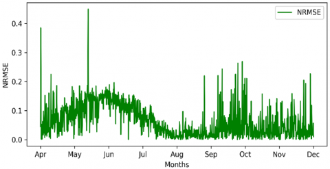
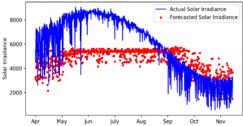
4.1.3 Monthly forecasting
Working with data as a 30-day window may give better performance, as shown in Figure 5, the forecast data curve is moving closer to the real data.
Figure 5. Window of 30
And the overall NRMSE is 0.188 with the curve as in Figure 6.
Figure 6. Window of 30-NRMSE
4.1.4 Weekly forecasting
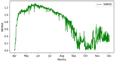
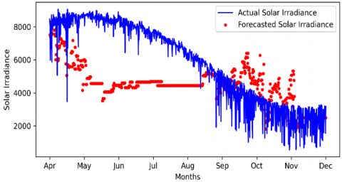
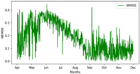
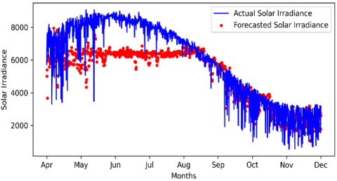
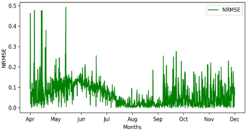
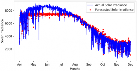
Working with solar power data needs more accurate steps. To do that, the window is defined to have 7 days for each, and the results curve is as in Figure 7.
Figure 7. Window of 7
The generated RMSE was 0.1672 with the curve shown in Figure 8.
Figure 8. Window of 7-NRMSE
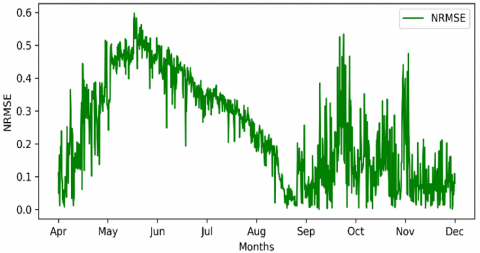
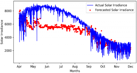
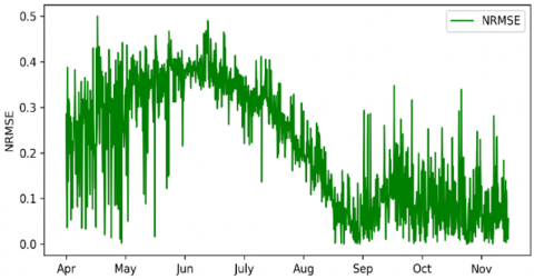
4.1.5 Two days forecasting
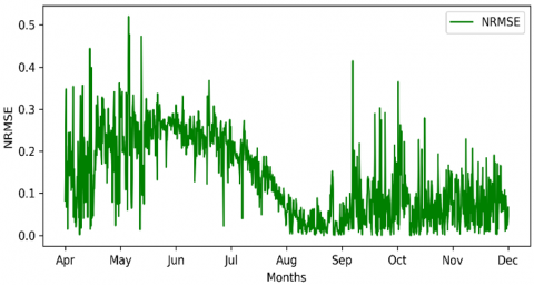
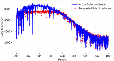
For one one-week window couldn’t give accurate results, a two-day model was implemented (the smallest possible window) to decide which window size is better. Window size 2 is shown in Figure 9.
Figure 9. Window of 2
As we move closer to real data, it is normal to have better RMSE results, with an overall NRMSE of 0.0926; the NRMSE curve is shown in Figure 10, which still provides highly loss forecasting, so a multi-condition was taken next.
Figure 10. Window of 2-NRMSE
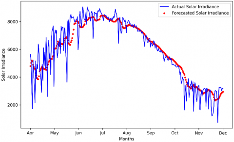
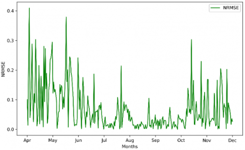
In addition, other weather parameters are taken to forecast irradiance, Pressure, Wind speed, Wind direction, Rainfall, Snowfall, Snow depth, and Relative Humidity can give a good idea about the solar irradiance state. The results are shown in Figure 11.
Figure 11. Window 2 with multiple conditions
With NRMSE 0.0855, which represents the best results from another implementation, with the NRMSE curve shown in Figure 12.
Figure 12. Window 2 with multiple condition-NRMSE
4.1.6 LightGBM forecasting
For comparison, another Gradient boosting method is used. This method is used with its basic hyper-parameters and without rolling window resizing; the hyper-parameters are set after using Python cross-validation code for best performance. The hyperparameters were bagging-fraction 0.8, bagging-freq 5, boosting-type dart, feature-fraction 0.8, learning-rate 0.1, max-depth 3, min-child-samples 20, and num-leaves: 31. The boosting-type type set to dart to overcome the over-fitting. The results are visualized in Figure 13.
Figure 13. LightGBM performance
Although it is a new method, in solar irradiance for casting, it is clear that the LightGBM model has poor results compared to our method, with an overall NRMSE = 0.2509, with an annual curve shown in Figure 14.
Figure 14. LightGBM-NRMSE
4.1.7 LSTM
This model represents the traditional solution for long-term forecasting. The model used contains two layers are applied with a dropout layer of 25% for each layer to reduce overfitting with the ADAM optimizer and an early stopping function. The output is introduced in Figure 15.
Figure 15. LSTM performance
From Figure 15, it is clear that the model tries to have the average of the values, which can lead to inaccurate results, with an average of 0.103. The NRMSE over time is shown in Figure 16.
Figure 16. LSTM-NRMSE
4.2 Discussion
Applying a rolling window enabled the model to focus on specific temporal segments of the data. Using a window size of 365 represents one forecaster for a year, 180, 30, which means having 12 forecasters in one year, 7, and 2 as shown in Table 1, gave a good view of how the implemented models operate with solar irradiance data:
Table 1. Windows size vs. metric performance
|
Method |
NRMSE |
MAE |
R2 |
Time in Seconds |
|
Window = 365 |
0.830 |
6159.701 |
-7.60 |
0.78 |
|
Window = 180 |
0.320 |
2262.58 |
-0.23 |
0.78 |
|
Window = 30 |
0.188 |
1319.007 |
0.55 |
0.89 |
|
Window = 7 |
0.167 |
1146.667 |
0.645 |
1.022 |
|
Window = 2 |
0.093 |
570.222 |
0.890 |
1.131 |
|
Window = 2 with weather parameters |
0.086 |
546.627 |
0.907 |
1.656 |
|
LightGBM |
0.251 |
1809.760 |
0.160 |
1.274 |
|
LSTM |
0.103 |
731.850 |
0.864 |
8.993 |
Table 1 indicates that larger window sizes reduce computational time but result in lower accuracy. Conversely, smaller window sizes necessitate more computational operations, increasing processing time, but provide higher model accuracy. The NRMSE values further reflect model performance. For instance, a window size of 2, combined with weather parameters, achieved lower error rates but required significantly more time to execute. However, the LightGBM model exhibited a higher NRMSE alongside greater processing times, highlighting its inefficiency in this context. For the optimal window size of 2, the impact of features is explained in two cases:
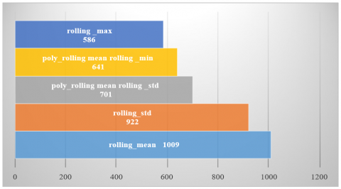
XGBoost features: rolling window statistics, which have the highest impact on the forecasting, are illustrated in Figure 17.
As shown in Figure 17, the rolling mean and rolling standard deviation (which are taken from previous iterations) have the greatest effect on the last forecast.
Figure 17. Features importance of rolling windows statistics in XGBoost
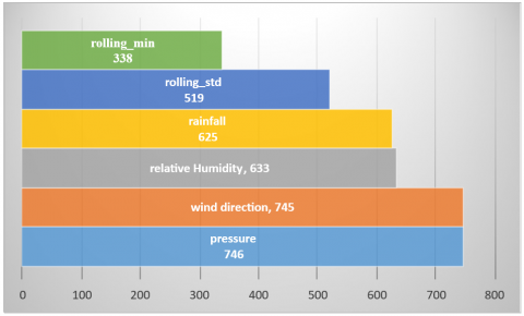
XGBoost and weather features: besides XGBoost features, weather parameters are added to the model, as shown in Table 1, which gives more accurate results. The parameters that have a higher impact on results are shown in Figure 18.
Figure 18. Combined importance of weather parameters in XGBoost
The figure demonstrates that, alongside weather parameters, XGBoost features such as rolling standard deviation and rolling minimum play critical roles in forecasting solar irradiance. The 'feature force' used in Figures 17-18 refers to the internal feature gain metric computed by the XGBoost model, rather than SHAP values. While SHAP provides a unified measure of feature impact, it was not used in this study. Future work will incorporate SHAP-based interpretability and structured ablation studies to better isolate the impact of individual weather features.
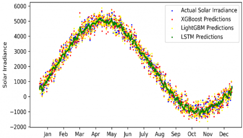
Unlike XGBoost, these methods lack the capability to segment datasets into smaller windows. Due to the inherent non-linearity of solar irradiance data, the results will be poor compared to the implemented XGBoost, as shown in Figure 19.
Figure 19. Comparative forecasting performance of XGBoost, LightGBM, and LSTM models
Figure 19 clarifies how the XGBoost predicted values are closer to the actual data than LightGBM and LSTM, which need more training and more computational efforts to have better results.
In summary, XGBoost achieved superior forecasting accuracy with an NRMSE of 0.0855, MAE of 273.4, and R² of 0.93, outperforming both LightGBM and LSTM across multiple window sizes. The 2-day window has lowest error rates, but its application may risk overfitting and is more sensitive to noise. While the findings reinforce the potential of small windows for short-term solar prediction, their use in long-term or real-time systems demands careful consideration of stability, scalability, and regional variability.
The finding of this paper has important implications for solar energy systems, especially in microgrid management and optimization. By showing the impact of window size on the performance of XGBoost models, the study provides a valuable insight for energy planners and engineering personnel. Whereas, selecting the optimal window size as shown in Table 1 is vital for the accuracy of solar irradiance forecasting along with computational efficiency in the real-time micro-grid workstation. The larger window size reduces computational load, but at the cost of prediction accuracy and vice versa. Lastly, the goal is to improve the reliability and efficiency of solar power generation, leading to a greater integration of renewable energy sources into global energy grids. By handling these practical considerations, this study contributes to the development of a more robust and dynamic solar energy infrastructure.
The improved performance observed with shorter windows, particularly the 2-day configuration, aligns with the highly non-stationary nature of solar irradiance patterns. However, shorter windows may lead to overfitting, especially when seasonality or long-term dependencies are ignored. From a practical standpoint, smaller windows require more frequent model retraining, increasing computational cost. Moreover, their generalization capability across different regions or high-frequency datasets may be limited, necessitating further validation in real-time systems.
The scope of this study was limited to evaluating the effect of rolling window sizes on XGBoost and comparing its performance to baseline LightGBM and LSTM models implemented with standard configurations. Applying rolling window techniques to LightGBM and LSTM, as well as conducting formal statistical significance tests such as paired t-tests to confirm the observed improvements, were beyond the scope of this work and are planned as part of future research. Additionally, future work may incorporate SHAP analysis to provide more precise and interpretable estimates of feature contributions, enhancing the understanding of how input variables influence model predictions. These extensions will provide a more comprehensive evaluation and strengthen the conclusions regarding the impact of windowing on different forecasting models.
Using a smaller window size in the XGBoost method is an effective way to improve the forecast results, although it takes a longer time; it can be implemented for nonlinear phenomena and long-term applications. Adding more weather parameters reduces the error range, even if the overall NRMSE is slightly larger, making the error smaller. Employing newer gradient boosting methods does not guarantee superior performance. For instance, LightGBM showed comparatively lower accuracy in long-term solar forecasting. With a relatively long time. For future work, it is possible to use other machine learning methods with XGBoost to build a hybrid model to improve the XGBoost model and make the forecast method closer to the real data. Building a long-term model for solar irradiance faces many challenges, and over-fitting one of them may give a faulty prediction, so future work can overcome it using statistical and other machine learning methods. Future work should also explore applying windowing to other models, including statistical significance tests, and adopt SHAP analysis to strengthen the interpretability and reliability of the results.
The authors gratefully acknowledge the use of the service and facilities of Ninevah University, Mosul University, and Al-Noor University. This study was funded by Al-Noor University, Iraq (Grant No.: ANU/2025/Eng.01).
[1] Hussain, Z., Dallalbashi, Z., Alhayali, S. (2021). Reviews of using solar energy to cover the energy deficit after the recent war in Mosul City. In International Conference on Data Science, E-Learning and Information Systems 2021, Petra, Jordan, pp. 254-265. http://doi.org/10.1145/3460620.3460766
[2] Al-Khazzar, A.A.A., Khaled, A.J. (2017). A comparative study of the available measured global solar radiation in Iraq. Journal of Renewable Energy and Environment, 4(2&3): 47-53. https://doi.org/10.30501/jree.2017.86011
[3] Chaichan, M.T., Kazem, H.A. (2018). Generating Electricity Using Photovoltaic Solar Plants in Iraq. Springer Cham, pp. 47-82. http://doi.org/10.1007/978-3-319-75031-6
[4] Al-Kayssi, A.A., Abdulrazzaq, O.A., Hamad, N.T. (2018). Analyzing of global solar radiation over Baghdad. International Journal of Science and Research, 7(9): 306-308. http://doi.org/10.21275/ART20191025
[5] Obiora, C.N., Ali, A., Hasan, A.N. (2021). Implementing extreme gradient boosting (XGBoost) algorithm in predicting solar irradiance. In 2021 IEEE PES/IAS PowerAfrica, Virtually, pp. 1-5. http://doi.org/10.1109/PowerAfrica52236.2021.9543159
[6] Yang, D., Kleissl, J., Gueymard, C.A., Pedro, H.T., Coimbra, C.F. (2018). History and trends in solar irradiance and PV power forecasting: A preliminary assessment and review using text mining. Solar Energy, 168: 60-101. http://doi.org/10.1016/j.solener.2017.11.023
[7] Mohamed, M., Mahmood, F.E., Abd, M.A., Rezkallah, M., Hamadi, A., Chandra, A. (2023). Load demand forecasting in smart microgrid using NWP via feature engineering. In 2023 IEEE International Conference on Energy Technologies for Future Grids, Wollongong, Australia, pp. 1-6. http://doi.org/10.1109/ETFG55873.2023.10408549
[8] Sulaiman, A., Mahmood, F.E., Majeed, S.A. (2023). Long-term solar irradiance forecasting using multilinear predictors. International Journal of Electrical and Electronic Engineering and Telecommunications, 12(2): 134-141. http://doi.org/10.18178/ijeetc.12.2.134-141
[9] Ali, B.M. (2023). Solar energy forecasting techniques based on machine learning: Survey. In 2023 6th International Conference on Engineering Technology and its Applications, Al-Najaf, Iraq, pp. 814-819. http://doi.org/10.1109/IICETA57613.2023.10351452
[10] Ali, B.M. (2023). Solar radiation estimation for renewable energy artificial intelligence. In 2023 6th International Conference on Engineering Technology and its Applications, Al-Najaf, Iraq, pp. 820-826. http://doi.org/10.1109/IICETA57613.2023.10351461
[11] Mohamed, M., Mahmood, F.E., Abd, M.A., Rezkallah, M., Hamadi, A., Chandra, A. (2023). Load demand forecasting using eXtreme gradient boosting (XGboost). In 2023 IEEE Industry Applications Society Annual Meeting, Nashville, United States, pp. 1-7. http://doi.org/10.1109/IAS54024.2023.10406613
[12] Gao, B., Huang, X., Shi, J., Tai, Y., Zhang, J. (2020). Hourly forecasting of solar irradiance based on CEEMDAN and multi-strategy CNN-LSTM neural networks. Renewable Energy, 162: 1665-1683. http://doi.org/10.1016/j.renene.2020.09.141
[13] Brahma, B., Wadhvani, R. (2020). Solar irradiance forecasting based on deep learning methodologies and multi-site data. Symmetry, 12(11): 1830. https://doi.org/10.3390/sym12111830
[14] Kumari, P., Toshniwal, D. (2021). Deep learning models for solar irradiance forecasting: A comprehensive review. Journal of Cleaner Production, 318: 128566. https://doi.org/10.1016/j.jclepro.2021.128566
[15] Kumari, P., Toshniwal, D. (2021). Long short term memory–Convolutional neural network based deep hybrid approach for solar irradiance forecasting. Applied Energy, 295: 117061. https://doi.org/10.1016/j.apenergy.2021.117061
[16] Huang, L., Kang, J., Wan, M., Fang, L., Zhang, C., Zeng, Z. (2021). Solar radiation prediction using different machine learning algorithms and implications for extreme climate events. Frontiers in Earth Science, 9: 596860. https://doi.org/10.3389/feart.2021.596860
[17] Bosilovich, M.G., Lucchesi, R., Suarez, M. (2015). MERRA-2: File specification. Technical Report. NASA, Washington D.C., USA.
[18] Wang, Z., Jia, L. (2020). Short-term photovoltaic power generation prediction based on LightGBM-LSTM model. In 2020 5th International Conference on Power and Renewable Energy, Shanghai, China, pp. 543-547. http://doi.org/10.1109/ICPRE51194.2020.9233298
[19] Bendali, W., Saber, I., Bourachdi, B., Amri, O., Boussetta, M., Mourad, Y. (2022). Multi time horizon ahead solar irradiation prediction using GRU, PCA, and GRID SEARCH based on multivariate datasets. Journal Européen des Systèmes Automatisés, 55(1): 11-23. https://doi.org/10.18280/jesa.550102
[20] Rajagukguk, R.A., Ramadhan, R.A., Lee, H.J. (2020). A review on deep learning models for forecasting time series data of solar irradiance and photovoltaic power. Energies, 13(24): 6623. https://doi.org/10.3390/en13246623
[21] Chen, T., Guestrin, C. (2016). Xgboost: A scalable tree boosting system. In Proceedings of the 22nd ACM SIGKDD International Conference on Knowledge Discovery and Data Mining, San Francisco, United States, pp. 785-794. https://doi.org/10.1145/2939672.2939785
[22] Hyndman, R.J., Athanasopoulos, G. (2018). Forecasting: Principles and Practice (3rd ed.). O Texts. https://otexts.com/fpp3/.
[23] Kumar, A.S., Reddy, V.U. (2023). Performance evaluation of Spider Web Te (S-B-T) PV panel configuration to reduce PV mismatch losses. Mathematical Modelling of Engineering Problems, 10(1): 383-387. https://doi.org/10.18280/mmep.100145
[24] Huang, X., Zhuang, X., Tian, F., Niu, Z., Chen, Y., Zhou, Q., Yuan, C. (2025). A hybrid ARIMA-LSTM-XGBoost model with linear regression stacking for transformer oil temperature prediction. Energies, 18(6): 1432. https://doi.org/10.3390/en18061432
[25] Ke, G., Meng, Q., Finley, T., Wang, T., et al. (2017). Lightgbm: A highly efficient gradient boosting decision tree. In Proceedings of the 31st International Conference on Neural Information Processing Systems, Long Beach, United States, pp. 3149-3157. https://doi.org/10.5555/3294996.3295074
[26] Elmnifi, M., Mhmood, A.H., Saieed, A.N.A., Alturaihi, M.H., Ayed, S.K., Majdi, H.S. (2024). A technical and economic feasibility study for on-grid solar PV in Libya. Mathematical Modelling of Engineering Problems, 11(1): 91-97. https://doi.org/10.18280/mmep.110109
[27] Wen, A., Wu, T., Wu, X., Zhu, X., et al. (2022). Evaluation of MERRA-2 land surface temperature dataset and its application in permafrost mapping over China. Atmospheric Research, 279: 106373. https://doi.org/10.1016/j.atmosres.2022.106373
[28] Draper, C.S., Reichle, R.H., Koster, R.D. (2018). Assessment of MERRA-2 land surface energy flux estimates. Journal of Climate, 31(2): 671-691. https://doi.org/10.1175/JCLI-D-17-0121.1
[29] Hinkelman, L.M. (2019). The global radiative energy budget in MERRA and MERRA-2: Evaluation with respect to CERES EBAF data. Journal of Climate, 32(6): 1973-1994. http://doi.org/10.1175/JCLI-D-18-0445.1