Moses Odiagbe*![]() | Opeyemi Osanaiye
| Opeyemi Osanaiye![]() | Omotayo Oshiga
| Omotayo Oshiga![]()
© 2025 The authors. This article is published by IIETA and is licensed under the CC BY 4.0 license (http://creativecommons.org/licenses/by/4.0/).
OPEN ACCESS
The increasing number of automobiles on the highway has led to a major difficulty in municipal traffic management. Intelligent Transportation Systems (ITS) require dependable traffic prediction algorithms capable of providing accurate forecasts at numerous time steps. This research proposes an Enhanced-Graph Neural Network (E-GNN) technique for traffic prediction and has been explored to augment the traditional GNN and temporal dependencies in traffic networks. A multimodal input was deployed for the preprocessing of the input data with GNN-Layer. An additional data stream was integrated to influence the traffic flow. The approach leverages strategically positioned loop detector sensors on the road network as a means of harvesting real-world traffic data. The suggested E-GNN technique for the estimation of real-time traffic speed was developed using two separate actual traffic datasets, such as PeMS-BAY and METR-LA. The result obtained over time shows a significant improvement, as seen in the 15-minute ahead prediction; the RMSE of EGNN reduced by 26.25% when compared with the existing state-of-the-art techniques.
traffic management, prediction, traffic congestion, attention mechanism, graph convolution network and spatial-temporal dependencies
Traffic sensor technology has transformed the acquisition and analysis of extensive traffic data, allowing Intelligent Transportation Systems (ITS) to manage and strategize urban traffic efficiently [1]. Forecasting traffic flow is essential for congestion relief and enhancing air quality. Congestion in metropolitan areas will continue to increase unless the state- of- the art techniques is adopted to mitigate these challenges. In 2014, it was estimated that about 6.9 billion hours of travel and 3.1 billion gallons of gasoline, totaling $160 billion in expenditure, of which trucks account for about 28% of this expenditure [2].
The rapid expansion in automotive use has led to social concerns such as traffic congestion, energy consumption, accidents, and high carbon emissions [3]. ITS is regarded as a promising approach to address these difficulties, giving real-time information and optimizing traffic signal timings. An accurate traffic forecast is vital for the successful implementation of ITS, and researchers have developed numerous ways to estimate traffic status. These approaches can be divided into superficial machine learning techniques, statistical techniques, and deep learning techniques. The Auto-Regressive Integrated Moving Average (ARIMA) is a part of the Statistical techniques used in machine learning, which have been frequently employed for traffic prediction [4, 5]. However, traditional machine learning models and parameter-driven approaches have trouble with handling large amounts of data, which limits how well they can predict the future. Deep learning algorithms exhibit potential in analyzing extensive traffic data; nonetheless, they possess some limitations that hinder them from performing optimally. Time-series data, especially multivariate time-series data (MTS), is hard to collect and analyze, therefore requires more than one feature to accurately predict traffic flow. This article presents a technique to overcome these restrictions by generating temporal features, establishing traffic flow operational status features, utilizing various state variables, and introducing an Enhanced-Graph Neural Network (E-GNN) approach with an attention mechanism that prioritizes pertinent feature vectors over time steps. The model surpassed all the existing traditional techniques used in traffic prediction and control datasets in predictive accuracy. Furthermore, these approaches depend on steady data and can propagate errors in multistep prediction. It is established that the machine learning algorithms used in the time past such as Support Vector Machines (SVM) [6, 7], Artificial Neural Networks (ANN) [8], k-Nearest Neighbors (kNN) [9], Bayesian networks, XGBoost [10], and random forest, have shown promising improvements over other techniques such as the statistical model but manually selected features are heavily relied on, and have shallow architectures, making them less suitable for complex traffic prediction tasks. Deep learning models have attracted prominence in various field of study ranging from engineering, science, and social science with a high success rate during implementation as it relates to transportation sector. Various deep learning-based techniques have been developed to forecast futuristic traffic patterns using different criteria. Zhang et al. [11] adopted a based grid model, Zhang et al. [12] adopted a system of traffic congestion prediction in the transport network using stacked auto-encoders, but fail to evaluate the effect of other characteristics, including occupancy, volume, speed, and traffic flow. Ma et al. [13] advocated Convolutional Neural Network (CNN) for predicting traffic speed, but fail to evaluate the distortion of traffic from nearby roads. Dai et al. [14] employed a hybrid spatiotemporal graph attention technique to anticipate traffic flow by comprehending past traffic flow patterns from upcoming traffic data volume. A Deep Belief Network (DBN) based technique was created by Li et al. [15], although its scalability has not been validated. Long Short Term Memory (LSTM) has also been developed to account for temporal dependency of traffic data. Graph-based techniques have been developed to represent spatial traffic dependency. Varieties of hybrid systems have been developed to predict future traffic, such as merging CNN and auto-encoder to estimate traffic flow based on previous weather and traffic data. However, these studies have either evaluated spatial dependency or temporal dependency, omitting the effect of traffic from other surrounding roads.
To be more exact, some of the existing drawbacks are highlighted below:
(1) The characteristics of dynamic traffic flows are not visible due to uncertainty and non-linearity.
(2) The impact of random disturbances or responses to unforeseen events, such as accidents, within the traffic system are not addressed adequately.
(3) Dynamically selecting sensor data to forecast a target sensor's traffic conditions over an extended timeframe presents a significant challenge.
(4) Occupancy, traffic volume, and speed are ignored during traffic flow.
(5) Classification of vehicles is usually difficult to differentiate.
(6) To solve these research gaps, a deep learning-based technique has been created to accurately estimate traffic speed at different time steps. The approach adopted in this article uses an E-GNN with multimodal input and GNN layers coupled with the output layer as shown in Figure 1.
Figure 1. Overview of the system architecture
The main contributions of this research are itemized below.
(1) To develop a robust traffic flow prediction and congestion control using E-GNN techniques with the aim of exploring spatial-temporal behavior of traffic networks.
(2) A graphical approach for traffic congestion control is adopted as an optimization strategy.
(3) We have also used 5 baselines to benchmark our proposed work.
(4) We have carried out a based-performance evaluation using a real-world dataset and compared its efficacy to state-of-the-art baseline methods.
The remaining parts of this paper are divided into the following sections: Section 2 presents the related work. Section 3 presents the research methodology for the proposed study. In Section 4, the experimental results are presented together with a comparison of the baseline model. Section 5 presents the conclusion and recommendations of the research.
Prior research has employed diverse traffic network modeling techniques to assess and forecast traffic trends. Parametric statistical methods, such as the Autoregressive Integrated Moving Average Model (ARIMA), were extensively utilized by various authors in the past, however the model was not so effective in predicting traffic flow due to accuracy issue, and most prediction were based on assumption. Machine learning methodologies, including Support Vector Regression (SVR), Feed-forward Neural Networks (NN), were proposed for traffic data modeling as described in references [16-18]. The SVR uses historical data to train the model and obtain the relationship between the input and output, but not effective when big data is involved. Deep learning has established a novel paradigm for traffic modeling, driven by the increasing prevalence, accessibility, and volume of traffic data. Methods based on deep neural networks have demonstrated great accuracy in traffic estimation and prediction tasks, attributed to the abundance of traffic data. Recurrent Neural Networks (RNNs) have been widely employed in recent studies to describe the spatiotemporal dynamics of traffic. Convolutional Neural Networks (CNNs) enhance the spatial modeling proficiency of deep learning models through the integration of numerous layers of neural connections. The various approach used for traffic prediction is discussed below.
2.1 Deep learning method for traffic prediction
Deep learning algorithms have proven to be capable of capturing nonlinear spatiotemporal dynamics for traffic prediction. Since the first study, numerous neural network-based models, such as fuzzy, recurrent, convolutional, Deep Belief Networks, auto-encoders, and generative adversarial networks, have been utilized to predict traffic conditions. RNNs, including LSTM and GRU [19], have been extensively utilized for forecasting traffic speed, journey time, and flow. In recent years, several deep learning models, including bidirectional LSTM, deep LSTM, shared hidden LSTM, and nested LSTM [20-23], have emerged to effectively capture intricate temporal correlations for traffic prediction. Multi-stream deep learning algorithms have been examined for traffic forecasting issues. Traditional CNN-based methods, on the other hand, can't automatically deal with the traffic network's topology and physical.
2.2 Graph convolution networks for traffic prediction
Traffic networks are examined as graphs for dynamic shortest path routing, congestion assessment, and dynamic traffic allocation. Recent studies have extended neural networks to operate on arbitrarily structured graphs through the use of graph convolutional networks [24]. These networks utilize the adjacency matrix or Laplacian matrix [25], to represent the configuration of a graph. Multiple approaches, such as spectral graph convolution and diffusion graph convolution, have been developed for comprehensive traffic forecasting across networks. However, physical specialties of roadways are often disregarded. Referring to the spectral graph theory, the convolution layer function used to define the spectral domain GCN and semi-supervised GCN based was first introduced in references [26, 27].
2.3 Spatial temporal graph network for traffic prediction
Spatial-temporal Graph networks are generally based on RNN-based and CNN-based techniques [28]. RNN-based methods filter inputs and hidden states using graph convolution, while CNN-based approaches combine graph convolution with 1D gated convolution [29]. However, RNN-based approaches are inefficient for large sequences and can explode when paired with graph convolution networks. Both approaches need stacking layers or global pooling for computational efficiency.
2.4 Attention based model for traffic prediction
The attention model, based on the encoder-decoder concept, has been widely employed in numerous applications, including image caption generation, recommendation systems, and document classification. This work used a soft attention model to learn the importance of traffic information at every time and construct a context vector for future traffic forecasting tasks. The design approach involved calculating hidden states, scoring functions, and constructing the context vector. In this study, a multilayer perception was utilized as the scoring function, with characteristics calculating the weight of each concealed state based on the attention process [30].
This study seeks to forecast traffic conditions utilizing historical roadway data, including speed, flow, and density. The approach employs an unweighted graph $G=\{v, \varepsilon, \mathrm{Y}\}$ to represent the topological configuration of the road network, with each road designated as a node. The adjacency matrix A denotes the relationships among roads and is represented as $A \in R^{n \times n}$. At each time step, the graph G possesses a dynamic feature matrix $Y^{(t)} \in R^{N \times D}$, which is utilized interchangeably with graph signals. The objective is to learn a function f that can predict its subsequent T-step graph signals. The expression is stated below.
$\begin{gathered}{\left[\mathrm{Y}^{(t-S): t}, G\right] \xrightarrow{f} \mathrm{Y}^{(t+1):(t+T)}} \\ \mathrm{Y}^{(t-S): t} \in \mathrm{R}^{N \times D \times S} \text { and } \mathrm{Y}^{(t+1):(t+T)} \in \mathrm{R}^{N \times D \times T}\end{gathered}$ (1)
where, N denotes the number of nodes, Yt denotes the graph signal in a given time t, D denotes the number of each feature of the nodes assigned, and S denotes the step graph signal.
3.1 Overview of the system architecture
The system architecture involves preprocessing multimodal data, aligning it with the road network graph, and using GNN layers to process node features. Temporal attention processes uncover key patterns, while cross-modal attention assesses input from multiple sources. The output is routed via a forecasting module to predict future traffic conditions. Figure 1 shows the detailed system architecture of the proposed model.
a. Multi-modal input
This includes the road network topology that model the road network as a graph in which nodes signify intersections or road segments, and edges denote connectedness. Preliminary node attributes may encompass fixed roadway characteristics (lane count, velocity restrictions). It is represented as follows.
$G=\{v, \varepsilon, Y\}$ (2)
$v=\left\{v_1 \ldots v_n\right\}$ (3)
b. Pre-processing
The pre-processing of the multimodal input includes traffic data, encompassing historical and real-time metrics such as speed, volume, and occupancy for each roadway segment. Weather, wind, and speed at pertinent places. Event data, details regarding planned events (concerts, sporting events, road closures) that may affect traffic conditions. The expression is given below:
$\left\{\mathrm{Y}_1 \ldots \mathrm{Y}_{\mathrm{T}}\right\} \xrightarrow{\mathrm{E}-\mathrm{GNN}}\left\{\mathrm{Y}_{\mathrm{T}+1} \ldots \mathrm{Y}_{\mathrm{T}^{\prime}}\right\}$ (4)
c. GNN layer
These layers process the node features, aggregating information from surrounding nodes based on the graph structure and the learnt spatial attention weights.
d. Temporal attention mechanism
The temporal attention mechanism is essential for capturing temporal dependencies in traffic data as it is seen from the system architecture it is one of basic components that allows the model to dynamically assess the significance of various time steps in the multimodal input sequence when predicting future time steps. The sequential analysis of the operation mechanism is as follows:
1. The attention mechanism is composed of an encoder that creates an attention vector from the multimodal input. There is also a decoder that perform other functions. A query is produced at each time steps in the output sequence, the query is then compared with keys produced from each time step in the multimodal input. The correlation between the query and each key dictates the attention weight.
2. Attention Weights: Attention weights are generally computed using a compatibility function followed by a softmax function to guarantee that the weights total equals to.
3. Higher Weights indicate a higher temporal dependency between the output time step and the matching input time step.
4. Weighted Sum: The data from the input sequence are subsequently amalgamated using the computed attention weights as coefficients. This weighted total creates the output for the current time step, effectively focusing on the most relevant historical information.
By allowing the model to attend to different parts of the input sequence with varying degrees of importance, the temporal attention mechanism can capture complex non-linear temporal relationships and dependencies that might be missed by traditional sequential models like RNNs or LSTMs without attention. This is particularly relevant in traffic data because patterns might be influenced by factors from many time scales (e.g., recent traffic conditions, daily commuting patterns, weekly trends, seasonal variations).
e. Cross-modal attention
Attention layers that allow the GNN to weigh the influence of diverse data modalities is introduced in the system model. For example, during heavy rain, the weather data might be given increased importance in predicting traffic slowdowns.
f. The output of the GNN layers is routed via a forecasting module (e.g., a linear layer or an RNN) to predict future traffic conditions.
Other components include the Enhanced-GNN layer, which extends to the GNN, CGAT, and the RNN, as well as the output component.
3.2 Evaluation
This section provides a comparative analysis of the proposed Enhanced-GNN model using the evaluation metrics as defined in the expression below. Five baseline models were used to benchmark the performance metrics of the proposed study. A visualization procedure was carried out to ascertain the most performing models from the listed baseline model, such as HA, ARIMA, STGCN, SVR, GMAN. However, this article employs various evaluation criteria, including MAPE, MSE, RMSE, and MAE. The expression for the evaluation indicators is given below.
$R M S E=\sqrt{\frac{1}{n} \sum_{i=1}^n\left|\hat{y}-y_i\right|^2}$ (5)
$M S E=\frac{1}{n} \sum_{i=1}^n\left|\hat{y}-y_i\right|^2$ (6)
$M A E=\frac{1}{n} \sum_{i=1}^n\left|\hat{y}-y_i\right|$ (7)
$M A P E=\frac{100}{n} \sum_{i=1}^n \frac{\left|\hat{y}-y_i\right|}{y_i}$ (8)
(1) Data description
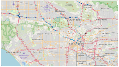
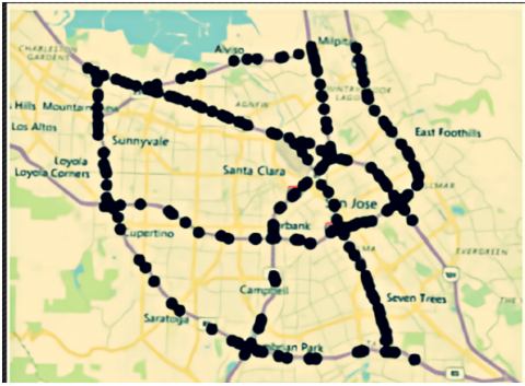
The research employs public traffic network datasets, such as the METR-LA and PEMS-BAY, used to examine traffic velocity across 207 sensors in Los Angeles County and 325 sensors in the Bay Area. The system approach was done using the following steps. First Data Mining or collection obtained from sensors that were strategically positioned. Followed by data pre-processing that was used as input to the GNN layer as explained earlier in Figure 1. Data pre-processing is analogous, involving 15-minute, 45minutes and 60 minutes intervals and the formulation of an adjacency matrix, the dataset were split into training, testing and validation. And final data visualization. However, the sensor arrangement is shown in Figures 2(a) and (b). The implementation was done using pytorch framework on an NVIDIA Ge-force. Three metrics were used to evaluate the traffic prediction task such as RMSE, MAPE, and MAE.
(a)
(b)
Figure 2. (a) PEMS_BAY: Sensor distribution; (b) METR_LA: Sensor distribution
(2) Baseline
We compare the E-GNN model to the following models: ARIMA, SVR, STGCN, GMAN and HA. Table 1 shows a brief description, advantages and disadvantages of the baseline model.
Table 1. Advantages and disadvantages of the baseline model
|
Model |
Advantage |
Disadvantage |
|
Autoregressive Integrated Moving Average (ARIMA) [31-33] |
•Mathematical simplicity and flexibility during application. •It is suitable for handling non-stationery time series. •High prediction accuracy. |
•The performance analysis and accuracy are based on assumptions. •The analysis is hindered by factors essential to the periodicity of the time series. •The relationships between upstream and downstream road sections are not accounted for during flow. |
|
History Average model (HA) [34] |
•For predicting data with periodic or seasonal patterns. •This approach uses the average traffic information in the historical periods as the prediction. |
•Prediction performance is limited. •The characteristics of dynamic traffic flows are not visible due to uncertainty and non-linearity. •The impact of random disturbances or responding to unforeseen events, such as accidents, within the traffic system is not adequately addressed. |
|
Graph Multi-Attention Network GMAN) [35] |
•They are adapted to encoder-decoder architecture. |
•Less effective due to the uncertainty and complexity of traffic flow. •Prone to error propagation. |
|
Support Vector Regression model (SVR) [36, 37] |
•This approach uses historical data to train the model and obtains the relationship between the input and output. •It is usually associated with high performance when data contains differentiable classes. •It works best when multidimensional data is involved and also when the dimension count is high. |
•Poor performance when big data sets are involved. •The accuracy is decreased drastically when noise occurs. •Prediction is usually low if the features are high in quantity as compared to the training samples. |
|
STGCN [38] |
•Used for binary classification. •Utilizes spatial structure for accurate traffic prediction. •It gives room for flexibility and scalability. |
•Accuracy issue may arise due to the large volume of data prediction. |
4.1 Experimental result
Table 2 illustrates the findings of the E-GNN model and other baseline models on the two datasets. The suggested strategy outperforms previous models with all three performance metrics on the two datasets. The ARIMA, SVR, STGCN, GMAN, and HA performance shows less performance as compared to the proposed model.
Table 2. Model comparison metrics
|
Dataset (METR-LA ) for 15 Minutes Horizon |
||||||
|
Metrics |
E-GNN |
ARIMA |
SVR |
STGCN |
GMAN |
HA |
|
RMSE |
6.3248 |
8.5763 |
8.7160 |
6.73310 |
6.50600 |
11.1164 |
|
MAPE (%) |
51.4249 |
106.7187 |
95.3148 |
51.8998 |
70.8160 |
77.4542 |
|
RAE |
0.1905 |
0.2567 |
0.2727 |
0.20750 |
0.19140 |
0.32970 |
|
Dataset (METR-LA) for 45 Minutes Horizon |
||||||
|
Metrics |
E-GNN |
ARIMA |
SVR |
STGCN |
GMAN |
HA |
|
RMSE |
9.5614 |
12.5417 |
11.6061 |
10.0595 |
9.92020 |
13.4029 |
|
MAPE (%) |
38.8570 |
50.9215 |
41.1729 |
39.8784 |
39.6356 |
51.1607 |
|
RAE |
0.3109 |
0.3684 |
0.36840 |
0.32310 |
0.31190 |
0.42230 |
|
Dataset (METR-LA) for 60 Minutes Horizon |
||||||
|
Metrics |
E-GNN |
ARIMA |
SVR |
STGCN |
GMAN |
HA |
|
RMSE |
10.2197 |
14.0377 |
12.9534 |
12.2384 |
11.6035 |
15.3673 |
|
MAPE (%) |
39.9670 |
50.4618 |
75.8591 |
49.4634 |
47.4973 |
88.2344 |
|
RAE |
0.3219 |
0.4424 |
0.39100 |
0.38770 |
0.35810 |
0.48180 |
|
Dataset (PEMS-BAY) for 15 Minutes Horizon |
||||||
|
Metrics |
E-GNN |
ARIMA |
SVR |
STGCN |
GMAN |
HA |
|
RMSE |
4.9399 |
7.6873 |
6.8468 |
5.9750 |
5.5531 |
8.7766 |
|
MAPE (%) |
19.6292 |
27.6847 |
33.1157 |
27.6489 |
22.2299 |
34.6893 |
|
RAE |
0.1985 |
0.3107 |
0.2732 |
0.2456 |
0.2297 |
0.3499 |
|
Dataset (PEMS-BAY) for 45 Minutes Horizon |
||||||
|
Metrics |
E-GNN |
ARIMA |
SVR |
STGCN |
GMAN |
HA |
|
RMSE |
7.1413 |
10.2669 |
8.8384 |
7.9819 |
7.3793 |
10.8666 |
|
MAPE (%) |
34.7723 |
47.7327 |
41.0162 |
39.1537 |
36.3425 |
53.8883 |
|
RAE |
0.2752 |
0.3991 |
0.3409 |
0.3193 |
0.2850 |
0.4266 |
|
Dataset (PEMS-BAY) for 60 Minutes Horizon |
||||||
|
Metrics |
E-GNN |
ARIMA |
SVR |
STGCN |
GMAN |
HA |
|
Metrics |
7.9691 |
11.7624 |
10.5428 |
9.1172 |
8.3929 |
11.8159 |
|
RMSE |
42.9535 |
49.0580 |
45.0392 |
49.5450 |
49.5450 |
48.3767 |
|
MAPE (%) |
0.3141 |
0.4723 |
0.4324 |
0.3729 |
0.3421 |
0.4738 |
|
RAE |
7.9691 |
11.7624 |
10.5428 |
9.1172 |
8.3929 |
11.8159 |
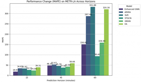
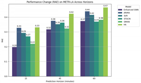
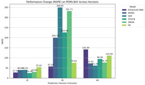
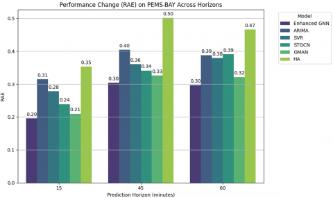
Particularly, the E-GNN algorithms that prioritize the modelling of this proposed work have superior prediction accuracy relative to the baseline models. The results indicate that the EGNN algorithm surpasses all other approaches across all error metrics for every prediction horizon. As seen in the 15 munites, 45 munites and 60 munites horizon, the RMSE error of EGNN is reduced by 26.25% as compared to ARIMA, 27.43% reduced as compared to SVR, 6.06% reduced as compared to STGCN, 2.78% reduced as compared to GMAN, and 43.10% as compared to HA. The other baseline model, although the error metrics of all models grow at the 45munites and 60munites horizons, EGNN models exhibit superior predictive performance relative to the baselines.
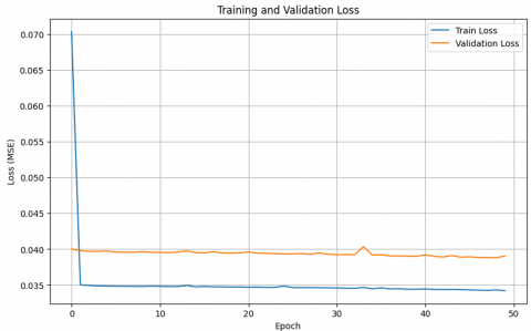
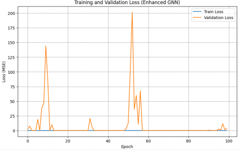
The proposed models were analysed using two learning curves, as depicted in Figures 3(a) and (b), one for each model, created based on the optimum parameters of the model. The training learning curve was derived from the loss of the training dataset, whereas the validation curve was derived from the validation dataset. The E-GNN algorithm exhibited the minimal validation and training error, signifying enhanced performance throughout the training phase. Both validation and training losses fell to a point of stability.
(a)
(b)
Figure 3. (a) Training and validation loss for the E-GNN for 50 epochs; (b) Training and validation loss for the E-GNN for 100 epochs as a reference point
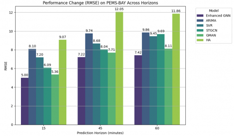
Figures 4(a)-(c) and Figures 4(d)-(f) illustrate the various prediction performances as compared to other models across various horizons on METR-LA and PEMS-BAY, respectively.
(a)
(b)
(c)
(d)
(e)
(f)
Figure 4. (a) Performance change (RMSE) on METR-LA across horizon; (b) Performance change (MAPE) on METR-LA across horizon; (c) Performance change (RAE) on METR-LA across horizon; (d) Performance change (MAPE) on PEMS-BAY across horizon; (e) Performance change (RAE) on PEMS-BAY across horizon; (f) Performance change (RMSE) on PEMS-BAY across horizon
In this paper, we proposed traffic prediction control model known as E-GNN as an improved method of solving traffic congestion related issues. The suggested model's performance was assessed via experimental analysis and compared with the current state-of-the-art models. As seen from the result, it is observed that our proposed model outperforms other models by a significant reduction in training loss. Comprehensive experimental evaluations were performed utilizing substantial, real-world datasets. The suggested E-GNN technique for the estimation of real-time traffic speed was developed using two separate actual traffic datasets, PeMS-BAY and METR-LA. It was also noticed from the experimental investigation that using both datasets for evaluating the performance metrics such as MAPE, RMSE, and MAE, errors significantly reduce with the increasing iteration count, which proved the viability, dependability, and practicability of the proposed approach. In the future research work we will explore the use of E-GNN for energy management and forecasting.
[1] Guerrero-Ibáñez, J., Zeadally, S., Contreras-Castillo, J. (2018). Sensor technologies for Intelligent Transportation Systems. Sensors, 18(4): 1212. https://doi.org/10.3390/s18041212
[2] Raymundo, H., dos Reis, J.G.M. (2019). Passenger transport disutilities in the US: An analysis since 1990s. In IFIP International Conference on Advances in Production Management Systems, Austin, TX, USA, pp. 118-124. https://doi.org/10.1007/978-3-030-29996-5_14
[3] Hofer, C., Jäger, G., Füllsack, M. (2018). Large scale simulation of CO2 emissions caused by urban car traffic: An agent-based network approach. Journal of Cleaner Production, 183: 1-10. https://doi.org/10.1016/j.jclepro.2018.02.113
[4] Gargari, N.S., Panahi, R., Akbari, H., Ng, A.K. (2022). Long-term traffic forecast using neural network and seasonal autoregressive integrated moving average: Case of a container port. Transportation Research Record, 2676(8): 236-252. https://doi.org/10.1177/03611981221083311
[5] Shuvo, M.A.R., Zubair, M., Purnota, A.T., Hossain, S., Hossain, M.I. (2021). Traffic forecasting using time-series analysis. In 2021 6th International Conference on Inventive Computation Technologies (ICICT), Coimbatore, India, pp. 269-274. https://doi.org/10.1109/ICICT50816.2021.9358682
[6] Toan, T.D., Truong, V.H. (2021). Support vector machine for short-term traffic flow prediction and improvement of its model training using nearest neighbor approach. Transportation Research Record, 2675(4): 362-373. https://doi.org/10.1177/0361198120980432
[7] Reddy, M.R., Sriramya, P. (2025). Traffic flow forecasting using support vector machine and comparing prediction accuracy with linear regression. AIP Conference Proceedings, 3270(1): 020055. https://doi.org/10.1063/5.0262833
[8] Kim, B., Baek, Y. (2020). Sensor-based extraction approaches of in-vehicle information for driver behavior analysis. Sensors, 20(18): 5197. https://doi.org/10.3390/s20185197
[9] Shaikh, M.K., Palaniappan, S., Ali, F., Khurram, M. (2020). Identifying driver behaviour through obd-ii using android application. PalArch's Journal of Archaeology of Egypt/Egyptology, 17(7): 13636-13647.
[10] Lattanzi, E., Freschi, V. (2021). Machine learning techniques to identify unsafe driving behavior by means of in-vehicle sensor data. Expert Systems with Applications, 176: 114818. https://doi.org/10.1016/j.eswa.2021.114818
[11] Zhang, S., Li, S., Li, X., Yao, Y. (2020). Representation of traffic congestion data for urban road traffic networks based on pooling operations. Algorithms, 13(4): 84. https://doi.org/10.3390/a13040084
[12] Zhang, Z., Li, M., Lin, X., Wang, Y., He, F. (2019). Multistep speed prediction on traffic networks: A deep learning approach considering spatio-temporal dependencies. Transportation Research Part C: Emerging Technologies, 105: 297-322. https://doi.org/10.1016/j.trc.2019.05.039
[13] Ma, X., Dai, Z., He, Z., Ma, J., Wang, Y., Wang, Y. (2017). Learning traffic as images: A deep convolutional neural network for large-scale transportation network speed prediction. Sensors, 17(4): 818. https://doi.org/10.3390/s17040818
[14] Dai, R., Xu, S., Gu, Q., Ji, C., Liu, K. (2020). Hybrid spatio-temporal graph convolutional network: Improving traffic prediction with navigation data. In KDD '20: Proceedings of the 26th ACM SIGKDD International Conference on Knowledge Discovery & Data Mining, Virtual Event, CA, USA, pp. 3074-3082. https://doi.org/10.1145/3394486.3403358
[15] Li, L., Qin, L., Qu, X., Zhang, J., Wang, Y., Ran, B. (2019). Day-ahead traffic flow forecasting based on a Deep Belief Network optimized by the multi-objective particle swarm algorithm. Knowledge-Based Systems, 172: 1-14. https://doi.org/10.1016/j.knosys.2019.01.015
[16] Lu, J., Zhang, X., Xu, Z., Zhang, J., Wang, J., Mao, L., Jia, L., Li, Z. (2020). Traffic index prediction and classification considering characteristics of time series based on autoregressive integrated moving average convolutional neural network model. Sensors Materials, 32(11): 3955-3973. https://doi.org/10.18494/SAM.2020.3058
[17] Nidhi, N., Lobiyal, D.K. (2022). Traffic flow prediction using support vector regression. International Journal of Information Technology, 14(2): 619-626. https://doi.org/10.1007/s41870-021-00852-2
[18] Ketkar, N., Moolayil, J. (2021). Feed-forward neural networks. In Deep Learning with Python. Apress, Berkeley, CA, pp. 93-131. https://doi.org/10.1007/978-1-4842-5364-9_3
[19] Fu, R., Zhang, Z., Li, L. (2016). Using LSTM and GRU neural network methods for traffic flow prediction. In 2016 31st Youth Academic Annual Conference of Chinese Association of Automation (YAC), Wuhan, China, pp. 324-328. https://doi.org/10.1109/YAC.2016.7804912
[20] Cui, Z., Ke, R., Pu, Z., Wang, Y. (2020). Stacked bidirectional and unidirectional LSTM recurrent neural network for forecasting network-wide traffic state with missing values. Transportation Research Part C: Emerging Technologies, 118: 102674. https://doi.org/10.1016/j.trc.2020.102674
[21] Duan, Y., Yisheng, L.V., Wang, F.Y. (2016). Travel time prediction with LSTM neural network. In 2016 IEEE 19th International Conference on Intelligent Transportation Systems (ITSC), Rio de Janeiro, Brazil, pp. 1053-1058. https://doi.org/10.1109/ITSC.2016.7795686
[22] Chen, Y.Y., Lv, Y., Li, Z., Wang, F.Y. (2016). Long short-term memory model for traffic congestion prediction with online open data. In 2016 IEEE 19th International Conference on Intelligent Transportation Systems (ITSC), Rio de Janeiro, Brazil, pp. 132-137. https://doi.org/10.1109/ITSC.2016.7795543
[23] Wu, Y., Tan, H. (2016). Short-term traffic flow forecasting with spatial-temporal correlation in a hybrid deep learning framework. arXiv preprint arXiv:1612.01022. https://doi.org/10.48550/arXiv.1612.01022
[24] Jia, Z., Wang, C., Wang, Y., Gao, X., Li, B., Yin, L., Chen, H. (2025). Recent research progress of graph neural networks in computer vision. Electronics, 14(9): 1742. https://doi.org/10.3390/electronics14091742
[25] Lutzeyer, J.F., Walden, A.T. (2017). Comparing graph spectra of adjacency and Laplacian matrices. In COMPLEX NETWORKS 2016: International Conference on Complex Networks and Their Applications, Milan, Italy, pp. 91-202. https://doi.org/10.1007/978-3-030-36683-4_16
[26] Kipf, T.N., Welling, M. (2016). Semi-supervised classification with graph convolutional networks. arXiv preprint arXiv:1609.02907. https://doi.org/10.48550/arXiv.1609.02907
[27] Bruna, J., Zaremba, W., Szlam, A., LeCun, Y. (2013). Spectral networks and locally connected networks on graphs. arXiv preprint arXiv:1312.6203. https://doi.org/10.48550/arXiv.1312.6203
[28] Bui, K.H.N., Cho, J., Yi, H. (2022). Spatial-temporal graph neural network for traffic forecasting: An overview and open research issues. Applied Intelligence, 52(3): 2763-2774. https://doi.org/10.1007/s10489-021-02587-w
[29] Malla, A.M., Banka, A.A. (2023). A systematic review of deep graph neural networks: Challenges, classification, architectures, applications potential utility in bioinformatics. arXiv preprint arXiv:2311.02127. https://doi.org/10.48550/arXiv.2311.02127
[30] Vijayalakshmi, B., Ramar, K., Jhanjhi, N.Z., Verma, S., Kaliappan, M., Vijayalakshmi, K., Vimal, S., Kavita, Ghosh, U. (2021). An attention-based deep learning model for traffic flow prediction using spatiotemporal features towards sustainable smart city. International Journal of Communication Systems, 34(3): e4609. https://doi.org/10.1002/dac.4609
[31] Kontopoulou, V.I., Panagopoulos, A.D., Kakkos, I., Matsopoulos, G.K. (2023). A review of ARIMA vs. machine learning approaches for time series forecasting in data driven networks. Future Internet, 15(8): 255. https://doi.org/10.3390/fi15080255
[32] Liu, R., Shin, S.Y. (2025). A review of traffic flow prediction methods in intelligent transportation system construction. Applied Sciences, 15(7): 3866. https://doi.org/10.3390/app15073866
[33] Ma, T., Antoniou, C., Toledo, T. (2020). Hybrid machine learning algorithm and statistical time series model for network-wide traffic forecast. Transportation Research Part C: Emerging Technologies, 111: 352-372. https://doi.org/10.1016/j.trc.2019.12.022
[34] Yao, H., Tang, X., Wei, H., Zheng, G., Li, Z. (2019). Revisiting spatial-temporal similarity: A deep learning framework for traffic prediction. Proceedings of the AAAI Conference on Artificial Intelligence, 33(1): 5668-5675. https://doi.org/10.1609/aaai.v33i01.33015668
[35] Zheng, C., Fan, X., Wang, C., Qi, J. (2020). GMAN: A graph multi-attention network for traffic prediction. Proceedings of the AAAI Conference on Artificial Intelligence, 34(1): 1234-1241. https://doi.org/10.1609/aaai.v34i01.5477
[36] Mesut, B., Başkor, A., Aksu, N.B. (2023). Role of artificial intelligence in quality profiling and optimization of drug products. In: A Handbook of Artificial Intelligence in Drug Delivery. Academic Press, pp. 35-54. https://doi.org/10.1016/B978-0-323-89925-3.00003-4
[37] Muthiah, H., Sa, U., Efendi, A. (2021). Support Vector Regression (SVR) model for seasonal time series data. In Proceedings of the Second Asia Pacific International Conference on Industrial Engineering and Operations Management, Surakarta, Indonesia, pp. 3191-3200.
[38] Yu, B., Yin, H., Zhu, Z. (2017). Spatio-temporal graph convolutional networks: A deep learning framework for traffic forecasting. In Proceedings of the Twenty-Seventh International Joint Conference on Artificial Intelligence (IJCAI-18), Stockholm, Sweden. https://doi.org/10.24963/ijcai.2018/505