Mustafa Mohammed Abdulrazaq*![]() | Vian N. Najm
| Vian N. Najm![]() | Athraa Mohammed S. Ahmed
| Athraa Mohammed S. Ahmed![]()
© 2025 The authors. This article is published by IIETA and is licensed under the CC BY 4.0 license (http://creativecommons.org/licenses/by/4.0/).
OPEN ACCESS
Resin 3-Dimensional (3D) printing technology moved beyond rapid prototyping to making of functional end-use products having intricate geometries and customized properties. MSLA (LCD-based) stereolithography provides higher levels of surface finish and dimensional accuracy, but it needs careful calibration of the parameters to find the right balance between mechanical performance and accuracy. The presented work explores the influence of exposure time, lifting speed and light-off delay on the compressive strength and the dimensional accuracy (diameter and height) of ASTM 695 samples. A full-factorial design of experiments has achieved to conduct the experiments that were analyzed using ANOVA. The results show that exposure duration is the most important element for compressive strength, accounting for about 62% of the total variation. Light-off delay, on the other hand, is the most important factor for dimensional integrity, accounting for about 45% of the variation in overall accuracy. The results show that there is a trade-off between mechanical performance and dimensional accuracy. Longer exposure times make the parts stronger but also make them a little oversized. On the other hand, an intermediate light-off delay of about 1.0 seconds gives the best dimensional accuracy. Featuring these insights, a multi-objective optimization framework using grey relational analysis was developed to find optimal parameter configuration that can achieve both high compressive strength and low dimensional errors.
LCD 3D printing, MSLA process, compressive strength, dimensional accuracy, grey relational analysis, multi-objective optimization
Additive Manufacturing (AM) is a revolutionary technique in modern manufacturing that can make complicated shapes with very little waste and tremendous material efficiency [1, 2]. Resin 3D printing techniques have gained popularity for their high-resolution 3D printing with fine details [3]. They are also known as photopolymerization techniques [4].
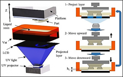
Stereolithography (SLA) and liquid crystal display (LCD)-based printing are two examples of vat photopolymerization processes that are highly recognized for their excellent precision and surface quality [5]. LCD 3D printing differs from DLP (Digital Light Processing) in that it utilizes a UV-light source that has been filtered via an LCD screen to cure photopolymer resins layer by layer, as shown in Figure 1 [6, 7]. More and more people have adopted this method for both prototyping and functioning applications because it is affordable and has a high feature resolution [8-10].
Figure 1. Schematic diagram of LCD printing [10]
ABS-like photopolymers are a common type of resin used in LCD 3D printing. They try to mimic how traditional Acrylonitrile Butadiene Styrene (ABS) behaves mechanically in standard manufacturing. These materials were chosen because they are rigid, strong, with simple fabrication and post-processing [11]. The proper selection of the process variables, like layer thickness, exposure duration, lifting speeds, and others, can have a big effect on how well printed parts behave mechanically (e.g., their compressive strength) and how accurately they fit together [12]. Various investigations have shown that the mechanical strength is a significant aspect of the quality of the fabricated objects, according to the relevant publications.
Brighenti et al. [13] conducted experiments and constructed theoretical models to find out how the mechanical characteristics of LCD printed photopolymers rely on the printing process parameters, which include the duration the UV light is on and the thickness of the layers. Through LCD 3D printing, Ahmed and Mugendiran [14] observed the process conditions that affect the mechanical qualities of PLA resin. By making the layers thicker and shortening the time between cures, you can get the most strength.
Diab et al. [15] explored how different printing parameters affect the tensile strength, strain, and Young's modulus of the printed parts using a Stereolithography machine. Their result revealed that the layer height, post curing time, and orientation affected the mechanical behavior of fabricated parts. Magalhães et al. [16] assessed the influence of the printing in different angular positions using cost effective LCD printer. Also, the samples were tested with three types of UV light curing resin in five different places on the printing platform. Their results showed that printing with inclined position had a significant effect on the printed parts quality.
Recent advancements in vat-photopolymerization underscore the need of multi objective optimization. Chekkaramkodi et al. [9] reviewed the significance of photopolymerization in the production of functional devices. Dhanunjayarao and Naidu [17] presented experimental findings for the dimensional accuracy of post cured samples fabricated by MSLA technique. They have reached the conclusion that a layer thickness of 0.06 mm constantly shows minimal variance for all of their results measures.
Unlike most investigations that concentrated on single-response optimization (e.g., strength or accuracy) for the thermoplastic-based additive manufacturing processes, the current work introduces an innovative application of Grey Relational Analysis to concurrently optimize both compressive strength and dimensional accuracy in LCD-printed ABS-like resins. To our knowledge, no prior study has systematically examined the cumulative impact of exposure duration, lift velocity, and light-off delay on this material system. This shows the contribution to the field and the novelty of the current research.
In order to explore the effect of exposure time, lifting speed, and Light-off delay on the process characteristics represented be the compressive strength and dimensional accuracy, three levels have been specified for each input variable as illustrated in Table 1. The parameters examined in this study were chosen due to their direct impact on resin curing dynamic and layer adherence in LCD printing. The other parameters, such as layer thickness and post-curing time, have been fixed to make sure they remained constant and to assure the stability of the process. To conduct the experimental runs, a full-factorial design has been adopted to obtain the input and output data through achieving a total of twenty-seven combinations designed by Minitab software.
Table 1. Printing factors and levels
|
No. |
Parameter |
Levels |
Unit |
||
|
(1) |
(2) |
(3) |
|||
|
1 |
Exposure Time |
1.8 |
2.2 |
2.6 |
s |
|
2 |
Lifting Speed |
40 |
60 |
80 |
mm/min |
|
3 |
Light-off Delay |
0.5 |
1 |
1.5 |
s |
2.1 Preparation, printing and testing
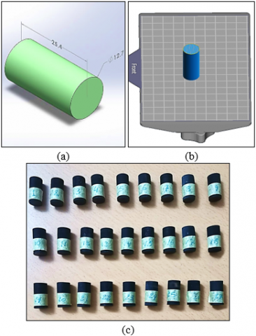
Based on the (ASTM695) standard, the compression test specimen was designed using SolidWorks software, shown in Figure 2(a). After making the part, the CAD model was saved in (.stl) format so that the slicer software could read it for slicing and setting the required printing conditions. For that purpose, Chitubox software was used to slice the CAD model into layers, make support structures, set the values for printing variables, and place the sample on the printer's surface in a virtual place as illustrated in Figure 2(b). To allow the printing machine to read the sliced file and create the desired geometry, the part must be saved as a G code file. The samples according to the various parameter combinations in the proposed design of experiments were printed using black ABS-Like resin on “Anycubic photon mono 6k” printer. After printing, all samples were put in a UV curing chamber (Anycubic Wash & Cure 2.0) for about 10 minutes at a wavelength of 405 nm. This standardised technique made guaranteed that the resin crosslinked in the same way, which reduced differences in mechanical and dimensional characteristics. Figure 2(c) clarify the twenty-seven printed samples.
Figure 2. Compression test specimen, (a) CAD model, (b) slicing the model, (c) printed parts
To reduce variability, all specimens were made from the same batch of ABS-like resin to avoid the variances in properties between batches. Before each set of prints, the resin was mixed well to make sure it was all the same, and the printer was recalibrated (build plate levelling and exposure test) to keep the process conditions the same. In addition, all samples were made in the same room temperature (25 ± 2℃). A preliminary statistical power analysis demonstrated that the selected full-factorial design with 27 runs, representing 3³ combinations, offered adequate degrees of freedom and experimental coverage to identify significant factor effects with a high level of confidence.
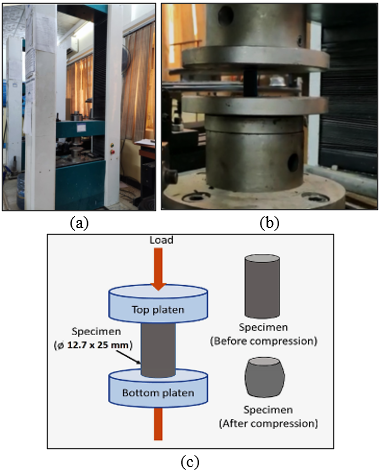
To perform a compression test on 3D-printed parts, a compressive force has to be applied to a sample and determine how well it resists the deformation. This test gives useful information for design and manufacturing by showing how strong, stiff, and how the material behaves under pressure. In the current work, the compression tests have been carried out for the fabricated ABS-like samples using a universal testing machine (WDW-50), shown in Figure 3(a). The specimen is placed on the lower jig and it is subjected slightly to compressive load by the upper jig with (1 mm/min) cross-head speed until the sample starts to deform by its shape or an unusual failure happens as illustrated in Figure 3(b). The testing setup for the compression test specimens is shown in Figure 3(c).
Figure 3. (a) Universal testing machine, (b) sample during test, (c) schematic diagram for compression test [18]
In additive manufacturing, making sure that dimensions are correct is very important, especially for mechanical testing applications like compression testing, where the exact shape affects how stress is spread and how valid the test is the study [19]. Changes from the nominal dimensions can cause stress concentrations or inconsistent loading circumstances, which can make strength measurements wrong and data untrustworthy [20]. So, checking the dimensional accuracy of printed parts is important to make sure that the printing process is accurate and that the specimens made are of good quality [5].
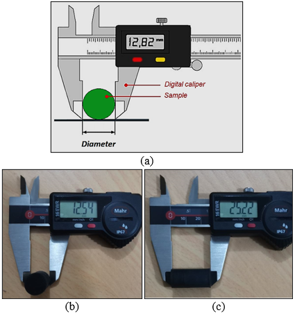
In the presented work, the dimensional accuracy of each cylindrical specimen has been checked by comparing the measured dimensions to their nominal CAD values. This was achieved by using a digital vernier calliper of a ±0.01 mm resolution to take the measurement and determine the dimensional correctness in this investigation. Microscopy or SEM imaging could give more information about the microstructure; however, the method used to measure be good enough to measure the geometric fidelity at the macro scale needed for compression testing. This indicates that dimensional deviations could be accurately measured without the need for advanced imaging.
For each specimen, the diameter at both the top and bottom boundaries has been measured to check for any changes that might have happened because of shrinkage or distortion. Also, the overall height along the vertical axis at two sites that were opposite each other has been measured. Afterwards, the average diameter and height were found and these numbers to figure out the dimensional correctness as a percentage. Figure 4 clarifies the measurement of the samples to compare the observed values to the notional CAD model and find out how accurate the dimensions are.
Figure 4. (a) Schematic of dimensional accuracy testing, (b) diameter measurement, (c) height measurement
This part illustrates and discusses the result of testing on the LCD-printed ABS-like parts’ compressive strength and dimensional accuracy. Table 2 shows the measured values of the responses. To keep the data presentation consistent, all of the numbers in the table were rounded to two decimal places.
The main focus of the examination is to clarify how the three main process parameters: exposure time, light-off delay, and lift speed affect the measured responses.
Main effects plot charts have been used to show how each parameter directly affects the compressive strength, the measured diameter, and the height. These charts show how particular levels of parameters affect specific performance measures and how the process reacts to changes in those levels. Also, the Analysis of Variance (ANOVA) on both the mechanical and dimensional responses to was used to figure out how important each of these factors is in relation to the others. This statistical method makes it possible to find the most important factors, showing which parameters have the biggest effect on the differences in compressive strength and accuracy that were seen. The combination of these graphs and statistics gives us a better understanding of the trade-offs between mechanical performance and dimensional fidelity. This is the basis for the multi-objective optimization technique provided in this paper.
Table 2. Experiments result of the compressive strength and dimensional accuracy
|
No. |
Et (s) |
Ls (mm/min) |
Loff (s) |
Compressive Strength (MPa) |
Accuracy |
|
|
Diameter Error% |
Height Error% |
|||||
|
1 |
1.80 |
40 |
0.50 |
37.21 |
-0.37 |
-0.30 |
|
2 |
1.80 |
40 |
1.00 |
48.43 |
0.71 |
0.80 |
|
3 |
1.80 |
40 |
1.50 |
46.58 |
0.46 |
-0.58 |
|
4 |
1.80 |
60 |
0.50 |
39.94 |
-0.69 |
-0.41 |
|
5 |
1.80 |
60 |
1.00 |
43.01 |
0.44 |
-0.84 |
|
6 |
1.80 |
60 |
1.50 |
42.26 |
0.12 |
0.40 |
|
7 |
1.80 |
80 |
0.50 |
36.08 |
-1.26 |
-0.92 |
|
8 |
1.80 |
80 |
1.00 |
42.57 |
0.25 |
-1.02 |
|
9 |
1.80 |
80 |
1.50 |
45.61 |
-0.28 |
-0.36 |
|
10 |
2.20 |
40 |
0.50 |
49.06 |
-0.11 |
-0.53 |
|
11 |
2.20 |
40 |
1.00 |
58.13 |
1.01 |
-0.06 |
|
12 |
2.20 |
40 |
1.50 |
51.38 |
0.39 |
0.18 |
|
13 |
2.20 |
60 |
0.50 |
43.03 |
-0.39 |
-0.35 |
|
14 |
2.20 |
60 |
1.00 |
51.53 |
0.46 |
-0.51 |
|
15 |
2.20 |
60 |
1.50 |
54.32 |
0.73 |
-0.35 |
|
16 |
2.20 |
80 |
0.50 |
45.76 |
-0.60 |
-1.33 |
|
17 |
2.20 |
80 |
1.00 |
48.72 |
0.73 |
-0.42 |
|
18 |
2.20 |
80 |
1.50 |
52.25 |
-0.01 |
-0.08 |
|
19 |
2.60 |
40 |
0.50 |
59.52 |
0.60 |
-0.51 |
|
20 |
2.60 |
40 |
1.00 |
67.99 |
0.90 |
0.65 |
|
21 |
2.60 |
40 |
1.50 |
65.01 |
0.85 |
0.71 |
|
22 |
2.60 |
60 |
0.50 |
51.08 |
0.39 |
-0.56 |
|
23 |
2.60 |
60 |
1.00 |
54.78 |
1.14 |
0.58 |
|
24 |
2.60 |
60 |
1.50 |
60.16 |
1.18 |
0.33 |
|
25 |
2.60 |
80 |
0.50 |
51.69 |
0.07 |
-0.27 |
|
26 |
2.60 |
80 |
1.00 |
55.52 |
0.40 |
-0.05 |
|
27 |
2.60 |
80 |
1.50 |
51.31 |
-0.24 |
0.56 |
3.1 Compressive strength results
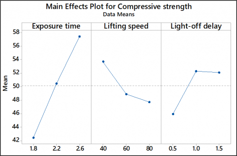
The main effect plots for the compressive strength illustrated in Figure 5 highlight that exposure time is the most important factor that affects how the printed samples behave mechanically. The compressive strength is raised when the exposure period goes from 1.8 seconds to 2.6 seconds. Longer UV exposure leads to increased photopolymerization and better interlayer adhesion, which makes the cross-linked polymer network denser and more cohesive. Light-off delay, on the other hand, had a small positive effect. By increasing the delay from 0.5 s to 1.5 s, the resin had more time to stabilise and level between layers. This made the surface less likely to have faults and made the compressive strength a little better. Lift speed had a relatively small effect compared to the other parameters. Very high lift speeds (80 mm/min) can cause too much peel force, which could lead to micro-defects or partial delamination between layers. However, the effect was not as strong as that of exposure time and light-off delay.
Figure 5. Main effects plot for the printed parts compressive strengths
The ANOVA results clarified in Table 3 verified this tendency, showing that exposure duration was responsible for about 63% of the difference in compressive strength, light-off delay for 15%, and lift speed for just 11%.
Table 3. ANOVA result of compressive strength
|
Source |
DOF |
Sum of Squares |
Variance |
F-value |
Contribution % |
|
Et |
2 |
1019.8 |
509.88 |
20.37 |
62.92 |
|
Ls |
2 |
180.5 |
90.24 |
1.5 |
11.14 |
|
Loff |
2 |
235.9 |
117.95 |
2.04 |
14.56 |
|
Error |
20 |
184.4 |
92.2 |
|
|
|
Total |
26 |
1620.6 |
|
|
|
Along with ANOVA, a regression analysis has been performed to ensure that exposure duration strongly affects compressive strength. The regression model validated that exposure time was the most significant, contributing to around 61-63% of the variation, which aligns with the ANOVA findings. It has been examined how the factors interacted with each other (Et × Ls, Et × Loff, Ls × Loff), whereas the results were not statistically significant. This shows that the primary effects are mostly responsible for the differences that have been observed, while interactions play only a little role.
3.2 Dimensional accuracy results
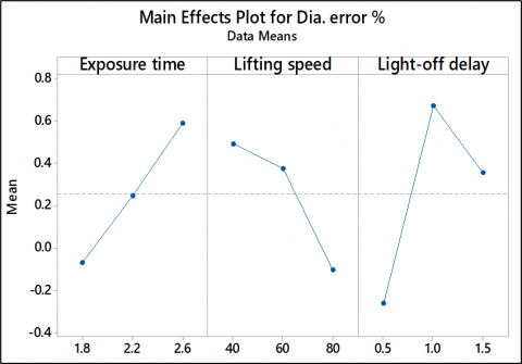
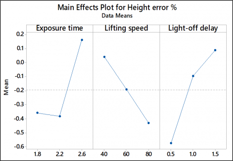
For the dimensional accuracy represented by the diameter and height error percentages, the influence of the parameters on the responses gave a considerably different from those for compressive strength, where light-off delay was the most important affecting parameter according to the ANOVA results shown in Table 4 and Table 5, with 43% and 25% for the diameter and height accuracy, respectively. As can be seen in the main effect plots illustrated in Figure 6, when the delay was increased from 0.5 s to 1.0 s, the dimensional accuracy improved. This was because the longer pause let the resin settle uniformly, which reduced undesired resin flow and made the layers more even. It's interesting that the accuracy went down a little as the delay went up to 1.5 s. This could be because the edges may have over-cured or the resin may have bled a little since it was exposed to ambient light for a longer period before the next layer was cured.
Table 4. ANOVA result of diameter accuracy
|
Source |
DOF |
Sum of Squares |
Variance |
F-value |
Contribution % |
|
Et |
2 |
1.933 |
0.967 |
3.09 |
20.47 |
|
Ls |
2 |
1.793 |
0.897 |
2.81 |
18.98 |
|
Loff |
2 |
4.065 |
2.032 |
9.06 |
43.03 |
|
Error |
20 |
1.656 |
0.828 |
|
|
|
Total |
26 |
9.447 |
|
|
|
Table 5. ANOVA result of height accuracy
|
Source |
DOF |
Sum of Squares |
Variance |
F-value |
Contribution % |
|
Et |
2 |
1.694 |
0.847 |
3.14 |
20.72 |
|
Ls |
2 |
1.003 |
0.501 |
1.68 |
12.26 |
|
Loff |
2 |
2.103 |
1.051 |
4.15 |
25.72 |
|
Error |
20 |
3.376 |
|
|
|
|
Total |
26 |
8.176 |
|
|
|
(a)
(b)
Figure 6. Main effects plot for the dimensional accuracy: (a) diameter error percentage, (b) height error percentage
Exposure duration had a secondary but important effect; longer exposure times (2.6 s) caused the sections to be a little oversized because they were over-polymerized at the edges. On the other hand, lower exposure (1.8 s) relatively undershot the dimensions because the boundaries didn't fully cure. Lift speed caused around 19% of the size differences. Slower speeds (40 mm/min) let the resin drain better and the layers line up better, while faster speeds (80 mm/min) caused little errors because of suction and peel forces.
The ANOVA results indicated somewhat elevated error contributions. This diversity can be ascribed to uncontrollable reasons, including slight fluctuations in resin temperature, light scattering inside the vat, and the intrinsic heterogeneity of photopolymer curing. Even though these factors may not be completely removed, the consistent experimental technique made sure that their effect remained acceptable.
Overall, the combination of diameter and height accuracies shows that light-off delay is the most important factor for managing dimensional fidelity. On the other hand, exposure time needs to be optimised to find the right balance between accuracy and mechanical strength. The current study measured dimensional accuracy through weighing up the errors in height and diameter. Both dimensions have a direct effect on the validity of compression testing, hence they were given equal weight. A sensitivity analysis demonstrated that modifying the weighting between diameter and height affected the optimization result by less than 5%, validating the resilience of this methodology.
The results of the mechanical and dimensional assessments together show how important it is to use a multi-objective optimisation technique for LCD 3D printing of ABS-like photopolymers. Longer exposure times improve compressive strength much strongly by increasing cross-link density, but they also tend to make dimensional accuracy worse by over-curing and edge expansion. On the other hand, the light-off delay mostly controls dimensional fidelity. Lift speed wasn't as important as other factors, but it nevertheless plays a part in reducing flaws caused by peeling and increasing the quality of the surface. These results show that no one factor can improve both mechanical performance and accuracy on its own. Instead, the trade-off area is defined by the interaction between exposure time (which is more important for mechanical strength) and light-off delay (which is more important for dimensional accuracy). This is where both attributes can be optimized at the same time. This understanding is the basis for the multi-objective optimization method used in this study, which tries to find parameter settings that give high compressive strength without losing dimensional accuracy.
3.3 Grey relational optimization
For optimizing the multiple printing characteristics that have been explored in the presented work, the Grey Relational Analysis (GRA) method was adopted to improve these outcomes simultaneously. GRA is a common method for solving multi-objective optimization problems, especially when the interactions between the variables are complicated or not fully recognized. This method transforms multiple performance factors into one grey relational grade (GRG), which allows to rank experimental conditions based on their overall quality of performance [21]. There are a number of steps in the GRA process. Firstly, normalisation is applied to bring all of the obtained values into a range that can be compared, usually between 0 and 1, depending on whether the response is "larger-the-better," "smaller-the-better," or "nominal-the-best." for the compressive strength case, the chosen criteria were larger is better using following equation [22]:
$y_i(k)=\frac{x_i(k)-\min x_{i(k)}}{\max x_i(k)-\min x_{i(k)}}$ (1)
where, $y_i(k)$ is $i^{\text {th}}$ normalized response value and $x_i(k)$ is the observed value for the $i^{\text {th}}$ run of the $k^{\text {th}}$ response. $\max x_i(k)$ and $\min x_i(k)$ are the maximum and minimum values across all experiments.
For the dimensional accuracy of the sample’s diameter and the height the criteria were nominal-the-best which can be expressed as:
$y_i(k)=1-\frac{\left|x_i(k)-x_{o(k)}\right|}{\max \left(\left|\max x_i(k)-x_0\right|,\left|\min x_i(k)-x_0\right|\right)}$ (2)
Next, the Deviation Sequence is generated, which indicates how far each normalised value is from the ideal (reference) value. A smaller deviation means that the performance in that area is better. The normalization data as well as the deviations sequence of the outputs are clarified in Table 6.
After that, the Grey Relational Coefficient (GRC) is calculated for each output using Eq. (3).
$\zeta_i(k)=\frac{\Delta_{\min}+\zeta \Delta_{\max}}{\Delta_i(k)+\zeta \Delta_{\max}}$ (3)
where, $\Delta_{\min}$ and $\Delta_{\max}$ are the global minimum and maximum values in different data series, respectively, for the $k^{\text {th}}$ response. The $\zeta_i(k)$ is the grey relational coefficient. The $\zeta$ is the distinguishing factor. GRC shows how close each possible outcome is to the best solution based on the deviation sequence and a differentiating factor, that is usually set to 0.5 [23].
After all, the GRG (Grey Relational Grade) represents the average of the GRCs for all of the outputs in each trial. The experiment with the highest GRG is the best combination to meet all of the goals. Table 7 illustrates the result of the calculations of the aforementioned steps to find the optimal parameter combination.
Table 6. Normalization and deviation sequence values
|
No. |
Responses |
Normalization |
Deviation Sequence |
||||||
|
Compressive Strength |
Diameter |
Height |
Compressive Strength |
Diameter |
Height |
Compressive Strength |
Diameter |
Height |
|
|
1 |
37.21 |
12.65 |
25.32 |
0.035 |
0.707 |
0.777 |
0.965 |
0.293 |
0.223 |
|
2 |
48.43 |
12.79 |
25.60 |
0.387 |
0.435 |
0.400 |
0.613 |
0.565 |
0.600 |
|
3 |
46.58 |
12.76 |
25.25 |
0.329 |
0.635 |
0.566 |
0.671 |
0.365 |
0.434 |
|
4 |
39.94 |
12.61 |
25.30 |
0.121 |
0.451 |
0.691 |
0.879 |
0.549 |
0.309 |
|
5 |
43.01 |
12.76 |
25.19 |
0.217 |
0.648 |
0.370 |
0.783 |
0.352 |
0.630 |
|
6 |
42.26 |
12.72 |
25.50 |
0.194 |
0.905 |
0.702 |
0.806 |
0.095 |
0.298 |
|
7 |
36.08 |
12.54 |
25.17 |
0.000 |
0.000 |
0.312 |
1.000 |
1.000 |
0.688 |
|
8 |
42.57 |
12.73 |
25.14 |
0.203 |
0.798 |
0.231 |
0.797 |
0.202 |
0.769 |
|
9 |
45.61 |
12.66 |
25.31 |
0.299 |
0.777 |
0.726 |
0.701 |
0.223 |
0.274 |
|
10 |
49.06 |
12.69 |
25.27 |
0.407 |
0.914 |
0.604 |
0.593 |
0.086 |
0.396 |
|
11 |
58.13 |
12.83 |
25.39 |
0.691 |
0.197 |
0.957 |
0.309 |
0.803 |
0.043 |
|
12 |
51.38 |
12.75 |
25.45 |
0.479 |
0.692 |
0.862 |
0.521 |
0.308 |
0.138 |
|
13 |
43.03 |
12.65 |
25.31 |
0.218 |
0.688 |
0.738 |
0.782 |
0.312 |
0.262 |
|
14 |
51.53 |
12.76 |
25.27 |
0.484 |
0.635 |
0.616 |
0.516 |
0.365 |
0.384 |
|
15 |
54.32 |
12.79 |
25.31 |
0.572 |
0.417 |
0.735 |
0.428 |
0.583 |
0.265 |
|
16 |
45.76 |
12.62 |
25.06 |
0.303 |
0.520 |
0.000 |
0.697 |
0.480 |
1.000 |
|
17 |
48.72 |
12.79 |
25.29 |
0.396 |
0.417 |
0.688 |
0.604 |
0.583 |
0.312 |
|
18 |
52.25 |
12.70 |
25.38 |
0.507 |
0.995 |
0.939 |
0.493 |
0.005 |
0.061 |
|
19 |
59.52 |
12.78 |
25.27 |
0.735 |
0.523 |
0.616 |
0.265 |
0.477 |
0.384 |
|
20 |
67.99 |
12.81 |
25.56 |
1.000 |
0.285 |
0.512 |
0.000 |
0.715 |
0.488 |
|
21 |
65.01 |
12.81 |
25.58 |
0.907 |
0.328 |
0.465 |
0.093 |
0.672 |
0.535 |
|
22 |
51.08 |
12.75 |
25.26 |
0.470 |
0.692 |
0.581 |
0.530 |
0.308 |
0.419 |
|
23 |
54.78 |
12.84 |
25.55 |
0.586 |
0.097 |
0.563 |
0.414 |
0.903 |
0.437 |
|
24 |
60.16 |
12.85 |
25.48 |
0.755 |
0.060 |
0.755 |
0.245 |
0.940 |
0.245 |
|
25 |
51.69 |
12.71 |
25.33 |
0.489 |
0.942 |
0.800 |
0.511 |
0.058 |
0.200 |
|
26 |
55.52 |
12.75 |
25.39 |
0.609 |
0.679 |
0.966 |
0.391 |
0.321 |
0.034 |
|
27 |
51.31 |
12.67 |
25.54 |
0.477 |
0.808 |
0.578 |
0.523 |
0.192 |
0.422 |
As can be noted in Table 7, experiment No. 18 has the optimal combination of printing parameters, namely, exposure time of 2.2 s, lifting speed of 80mm/min, and light of delay 1.5 mm/min. This particular approach is effective and appropriate when it's required to find a balance between contending outcomes, like making the printed parts stronger while keeping their dimensions accurate. Grey Relational Analysis (GRA) has been used over other multi-objective methods like TOPSIS because it can handle complicated interactions with little experimental data and makes it easy to rank combinations of parameters. This is why GRA is so useful for studies of additive manufacturing, since it is possible to look at the trade-offs between strength and precision at the same time.
Table 7. Grey Relational coefficient, grade and rank of optimal parameters
|
No. |
Responses |
Grey Relational Coefficient |
Grade |
Rank |
||||
|
Compressive Strength |
Diameter |
Height |
Compressive Strength |
Diameter |
Height |
|||
|
1 |
37.21 |
12.65 |
25.32 |
0.695 |
0.892 |
0.919 |
0.835 |
18 |
|
2 |
48.43 |
12.79 |
25.60 |
0.785 |
0.800 |
0.790 |
0.792 |
25 |
|
3 |
46.58 |
12.76 |
25.25 |
0.769 |
0.867 |
0.841 |
0.826 |
19 |
|
4 |
39.94 |
12.61 |
25.30 |
0.715 |
0.804 |
0.886 |
0.802 |
22 |
|
5 |
43.01 |
12.76 |
25.19 |
0.739 |
0.871 |
0.780 |
0.797 |
24 |
|
6 |
42.26 |
12.72 |
25.50 |
0.733 |
0.975 |
0.891 |
0.866 |
8 |
|
7 |
36.08 |
12.54 |
25.17 |
0.687 |
0.687 |
0.764 |
0.712 |
27 |
|
8 |
42.57 |
12.73 |
25.14 |
0.735 |
0.929 |
0.742 |
0.802 |
21 |
|
9 |
45.61 |
12.66 |
25.31 |
0.760 |
0.919 |
0.899 |
0.859 |
11 |
|
10 |
49.06 |
12.69 |
25.27 |
0.791 |
0.978 |
0.855 |
0.875 |
5 |
|
11 |
58.13 |
12.83 |
25.39 |
0.886 |
0.734 |
0.998 |
0.873 |
6 |
|
12 |
51.38 |
12.75 |
25.45 |
0.813 |
0.887 |
0.956 |
0.886 |
4 |
|
13 |
43.03 |
12.65 |
25.31 |
0.739 |
0.885 |
0.904 |
0.842 |
16 |
|
14 |
51.53 |
12.76 |
25.27 |
0.815 |
0.867 |
0.859 |
0.847 |
15 |
|
15 |
54.32 |
12.79 |
25.31 |
0.844 |
0.795 |
0.903 |
0.847 |
14 |
|
16 |
45.76 |
12.62 |
25.06 |
0.762 |
0.826 |
0.687 |
0.758 |
26 |
|
17 |
48.72 |
12.79 |
25.29 |
0.788 |
0.795 |
0.884 |
0.822 |
20 |
|
18 |
52.25 |
12.70 |
25.38 |
0.822 |
1.017 |
0.990 |
0.943 |
1 |
|
19 |
59.52 |
12.78 |
25.27 |
0.903 |
0.828 |
0.859 |
0.863 |
10 |
|
20 |
67.99 |
12.81 |
25.56 |
1.020 |
0.757 |
0.825 |
0.867 |
7 |
|
21 |
65.01 |
12.81 |
25.58 |
0.975 |
0.769 |
0.810 |
0.852 |
12 |
|
22 |
51.08 |
12.75 |
25.26 |
0.811 |
0.887 |
0.846 |
0.848 |
13 |
|
23 |
54.78 |
12.84 |
25.55 |
0.849 |
0.710 |
0.841 |
0.800 |
23 |
|
24 |
60.16 |
12.85 |
25.48 |
0.911 |
0.701 |
0.912 |
0.841 |
17 |
|
25 |
51.69 |
12.71 |
25.33 |
0.817 |
0.993 |
0.929 |
0.913 |
3 |
|
26 |
55.52 |
12.75 |
25.39 |
0.857 |
0.883 |
1.003 |
0.914 |
2 |
|
27 |
51.31 |
12.67 |
25.54 |
0.813 |
0.932 |
0.846 |
0.864 |
9 |
This study shows the intricate nature of the relationship between the variables of LCD printing and the mechanical and dimensional qualities of ABS-like resin parts. According to the results, it can be concluded that exposure duration has a significant impact on compressive strength because it directly affects cross-link density and interlayer adhesion. Light-off delay, on the other hand, mostly governs dimensional correctness by altering resin flow stability and curing uniformity. Lift speed is less important, but it does help reduce flaws and surface imperfections caused by peeling. The investigation showed that there is no one variable that can make both compressive strength and dimensional accuracy as high as possible at the same time. So, a multi-objective optimisation strategy using GRA method was performed to balance the main effect of exposure time (for compressive strength) and light-off delay (for accuracy) to find the best compromise. The findings of this investigation give useful advice on how to adjust LCD printing variables to make ABS-like components that are both strong and accurate in size, which is important for parts functionality and load bearing demand. These findings also give a recommendation for real-world LCD printing environments from a practical point of view. For functional or load-bearing parts, extended exposure times are suggested because they greatly increase compressive strength, even if this means that the pieces are slightly larger than they should be. On the other hand, for aesthetic pieces or sections where dimensional precision is really important, moderate exposure times and intermediate light-off delays (around 1.0 s) work better for accuracy without making the strength too weak. These trade-offs show that choosing parameters should be based on the application.
[1] Paral, S.K., Lin, D.Z., Cheng, Y.L., Lin, S.C., Jeng, J.Y. (2023). A review of critical issues in high-speed vat photopolymerization. Polymers, 15(12): 2716. https://doi.org/10.3390/polym15122716
[2] Abdulrazaq, M.M., AL-Khafaji, M.M.H., Kadauw, A. (2025). The influence of slicing parameters on mechanical strength of FDM printed parts: A review. AIP Conference Proceedings, 3169. https://doi.org/10.1063/5.0254289
[3] Bao, Y. (2022). Recent trends in advanced photoinitiators for vat photopolymerization 3D printing. Macromolecular Rapid Communications, 43(14): 2200202. https://doi.org/10.1002/marc.202200202
[4] Piedra-Cascón, W., Krishnamurthy, V.R., Att, W., Revilla-León, M. (2021). 3D printing parameters, supporting structures, slicing, and post-processing procedures of vat-polymerization additive manufacturing technologies: A narrative review. Journal of Dentistry, 109: 103630. https://doi.org/10.1016/j.jdent.2021.103630
[5] Ngo, T.D., Kashani, A., Imbalzano, G., Nguyen, K.T.Q., Hui, D. (2018). Additive manufacturing (3D printing): A review of materials, methods, applications and challenges. Composites Part B: Engineering, 143: 172-196. https://doi.org/10.1016/j.compositesb.2018.02.012
[6] Abdulrazaq, M.M., Najm, V.N., Ahmed, A.M.S. (2025). Optimizing the impact strength and hardness of the liquid crystal display printed parts using artificial neural network. Advances in Science and Technology Research Journal, 19(8): 373-383. https://doi.org/10.12913/22998624/205714
[7] Mele, M., Campana, G. (2022). Advancing towards sustainability in liquid crystal display 3D printing via adaptive slicing. Sustainable Production and Consumption, 30: 488-505. https://doi.org/10.1016/j.spc.2021.12.024
[8] Zhao, Z., Tian, X., Song, X. (2020). Engineering materials with light: Recent progress in digital light processing based 3D printing. Journal of Materials Chemistry C, 8(40): 13896-13917. https://doi.org/10.1039/D0TC03548C
[9] Chekkaramkodi, D., Jacob, L., Umer, R., Butt, H. (2024). Review of vat photopolymerization 3D printing of photonic devices. Additive Manufacturing, 86: 104189. https://doi.org/10.1016/j.addma.2024.104189
[10] Zhu, Z. (2023). Freeform optics for achieving collimated and uniform light distribution in LCD-type UV-curable 3D printing. IEEE Photonics Journal, 15(4): 1-7. https://doi.org/10.1109/JPHOT.2023.3294478
[11] Golubović, Z., Danilov, I., Bojović, B., Petrov, L., Sedmak, A., Mišković, Z., Mitrović, N. (2023). A comprehensive mechanical examination of ABS and ABS-like polymers additively manufactured by material extrusion and vat photopolymerization processes. Polymers, 15(21): 4197. https://doi.org/10.3390/polym15214197
[12] Batista, M., Mora-Jimenez, J., Salguero, J., Vazquez-Martinez, J.M. (2024). Assessment of the development performance of additive manufacturing VPP parts using digital light processing (DLP) and liquid crystal display (LCD) technologies. Applied Sciences, 14(9): 3607. https://doi.org/10.3390/app14093607
[13] Brighenti, R., Marsavina, L., Marghitas, M.P., Cosma, M.P., Montanari, M. (2023). Mechanical characterization of additively manufactured photopolymerized polymers. Mechanics of Advanced Materials and Structures, 30(9): 1853-1864. https://doi.org/10.1080/15376494.2022.2045655
[14] Ahmed, A.R., Mugendiran, V. (2024). Effect of process parameters on mechanical properties of PLA resin through LCD 3D printing. Proceedings of the Institution of Mechanical Engineers, Part E: Journal of Process Mechanical Engineering. https://doi.org/10.1177/09544089231225147
[15] Diab, R.R., Enzi, A., Hassoon, O.H. (2023). Effect of printing parameters and post-curing on mechanical properties of photopolymer parts fabricated via 3D stereolithography printing. IIUM Engineering Journal, 24(2): 225-238. https://doi.org/10.31436/iiumej.v24i2.2778
[16] Magalhães, F.C., Leite, W.O., Campos Rubio, J.C. (2024). A study of mechanical properties of photosensitive resins used in vat photopolymerization process. Journal of Elastomers and Plastics, 56(6): 807-829. https://doi.org/10.1177/00952443241256632
[17] Dhanunjayarao, B.N., Naidu, N.V.S. (2022). Assessment of dimensional accuracy of 3D printed part using resin 3D printing technique. Materials Today: Proceedings, 59: 1608-1614. https://doi.org/10.1016/j.matpr.2022.03.148
[18] Sivasankaran, S., Al-Mufadi, F. (2020). Influence of strain rate and percentage of cold work on room-temperature deformation behaviour of AISI 1015 carbon steel: Detailed microstructures and cold workability map investigations. Transactions of the Indian Institute of Metals, 73(6): 1439-1448. https://doi.org/10.1007/s12666-020-01901-3
[19] Goh, G.D., Yap, Y.L., Tan, H.K.J., Sing, S.L., Goh, G.L., Yeong, W.Y. (2020). Process-structure-properties in polymer additive manufacturing via material extrusion: A review. Critical Reviews in Solid State and Materials Sciences, 45(2): 113-133. https://doi.org/10.1080/10408436.2018.1549977
[20] ASTM International. (2015). Test Method for Compressive Properties of Rigid Plastics. ASTM D695-15. https://doi.org/10.1520/D0695-15
[21] Bhaumik, M., Maity, K. (2021). Multi-response optimization of EDM parameters using grey relational analysis (GRA) for Ti-5Al-2.5 Sn titanium alloy. World Journal of Engineering, 18(1): 50-57. https://doi.org/10.1108/WJE-06-2020-0210
[22] Daniel, S.A.A., Pugazhenthi, R., Kumar, R., Vijayananth, S. (2019). Multi objective prediction and optimization of control parameters in the milling of aluminium hybrid metal matrix composites using ANN and Taguchi-grey relational analysis. Defence Technology, 15(4): 545-556. https://doi.org/10.1016/j.dt.2019.01.001
[23] Sreejith, S., Priyadarshini, A., Chaganti, P.K. (2020). Multi-objective optimization of surface roughness and residual stress in turning using grey relation analysis. Materials Today: Proceedings, 26: 2862-2868. https://doi.org/10.1016/j.matpr.2020.02.594