Pragati Khare*![]() | Dipti Jadhav
| Dipti Jadhav![]()
© 2025 The authors. This article is published by IIETA and is licensed under the CC BY 4.0 license (http://creativecommons.org/licenses/by/4.0/).
OPEN ACCESS
Accurate and timely poverty estimation is fundamental for the formulation of effective policies aimed at eradicating poverty in accordance with Sustainable Development Goal 1 (SDG-1). Traditional methods such as censuses and household surveys, though widely adopted, are limited by infrequency, high costs, and potential reporting errors. In contrast, satellite-derived data offer scalable and cost-effective alternatives. In this study, district-level poverty in Madhya Pradesh, India, was estimated using a Deep Learning (DL) framework that leverages Night-Time Light (NTL) satellite imagery in conjunction with environmental variables—specifically the Air Quality Index (AQI) and radiance intensity. Two modeling strategies were employed. First, a baseline approach was implemented using a pre-trained Squeeze-and-Excitation Network (SENet) architecture to extract visual features from NTL imagery, followed by classification via three Machine Learning (ML) algorithms: Support Vector Machine (SVM), Random Forest (RF), and Extreme Gradient Boosting (XGBoost). Second, a modified SENet-154 model was developed by integrating structured environmental features (AQI and radiance) directly into the classification pipeline, enabling joint learning from both visual and environmental modalities. The modified SENet-154 model demonstrated superior predictive performance, achieving an overall classification accuracy of 93.60%. Spatial autocorrelation analysis, conducted using Local Indicators of Spatial Association (LISA), confirmed the geographical coherence of the predicted poverty clusters across districts, thereby validating the model's spatial reliability. The findings underscore the utility of NTL imagery as a proxy for socio-economic assessment and highlight the substantial gains in predictive accuracy obtained through the incorporation of environmental indicators. This integrative approach not only enhances the spatial granularity of poverty mapping but also emphasizes the interconnectedness of environmental degradation and economic deprivation. The results provide compelling evidence to support the design of policy interventions that concurrently address environmental sustainability and poverty alleviation.
SDGs, NTL imagery, AQI, radiance, MPI, DL, spatial analysis
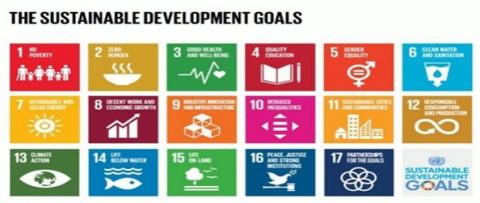
Economic well-being remains one of the most critical issues in socio-economic planning and policy-making, as it directly impacts resource allocation, welfare programs, and long-term development strategies. SDGs, led by the United Nations [1], aim to ensure prosperity for all by the year 2030. As illustrated in Figure 1, “no poverty” holds the first position in 17 SDGs.
Figure 1. SDGs by the United Nations [1]
Poverty is a multidimensional phenomenon characterized by the deprivation of basic human needs, including food, shelter, education, healthcare, and economic opportunity. It is commonly classified into two main types: absolute and relative poverty.
• Absolute poverty: A person living on less than $2.15 per day (2022 purchasing power parity) [2], as given by the World Bank.
• Relative poverty: Inequality compared to a society’s average standard of living by the United Nations’ Multidimensional Poverty Index (MPI), which defines poverty not only in terms of money but also in education, health, and living standards, highlighting disparities in access to clean water, electricity, and sanitation [3].
Timely estimation of poverty levels is the first step toward achieving SDG-1. The lack of real-time and accurate poverty estimation makes it difficult to implement timely interventions and assess the effectiveness of policies. Traditional methods for poverty estimation rely on national censuses and household surveys like demographic and health surveys which rely on collecting data from individuals. Manually analyzing collected data is time-consuming and not cost-effective. In a country like India, frequent surveys are often not feasible, especially in remote or conflict-affected regions. There is a recent advancement in the methods for measuring poverty. With the increasing usage of Remote Sensing (RS), Artificial Intelligence (AI) [4], and ML [5], various real-time and accurate data sources for analysis are available. Satellite imagery has emerged as a valuable proxy for assessing economic activity [6]. It provides indicators, such as urban expansion, road and building density, and night-time illumination, which reflect infrastructure growth, electricity access, and population distribution that in turn state the socio-economic conditions.
Environmental factors play a very important role in the day-to-day living and working conditions of people. Recently, these factors have emerged as important indicators of socio-economic status, particularly in regions where reliable ground-level data is not available. Variables such as air quality [7], NTL intensity [8], land use patterns, and vegetation indices like Normalized Difference Vegetation Index (NDVI) [9] offer insights into living conditions, infrastructure availability, and development levels. Poor air quality, low radiance, limited green cover, and proximity to environmental hazards often result in poor living conditions. By analyzing these spatial and environmental parameters, researchers state the disparities in access to resources, housing quality, and overall well-being, thus supporting data-driven poverty assessment in underserved or remote areas. While some studies have used NTL satellite data or environmental indicators independently for socio-economic prediction, limited research integrates both features. Moreover, few studies have validated these models through spatial correlation and regional relevance.
This research presents a novel study that integrates the capabilities of NTL satellite image data along with environmental features in estimating poverty levels. Out of the numerous environmental indicators explored in the literature, this study concentrates on AQI and radiance due to their strong correlation with urban infrastructure, economic activity, and public health. This study aims to:
• Assess the role of AQI and night-time radiance in enhancing the accuracy of poverty prediction models derived from satellite imagery.
• Evaluate the effect of integrating environmental variables on the classification performance of poverty levels.
• Validate the spatial consistency of predicted poverty clusters using spatial correlation techniques such as LISA.
Traditional data-gathering techniques like household surveys and census reports have long been used to predict and map poverty. These methods are time-consuming and resource-intensive and have a limited scope in terms of both space and time. With the introduction of new techniques to evaluate socio-economic situations using data-driven, scalable techniques because of the growing availability of RS data, especially NTL satellite imaging and environmental indicators like AQI, there is a major change in terms of poverty mapping.
A common proxy for economic expansion, urbanization, and human activity is NTL imaging. NTL images are indirect but important indicators of wellness, developed infrastructure, and resource accessibility, offering insights into human development observable at night. Recently, air quality has become an important factor in determining urban inequality and public health, particularly in areas that are quickly urbanizing. Research indicates a strong correlation between low-income communities and poor air quality, which makes AQI a possible environmental indicator of underdevelopment and poverty. This literature review examines significant research contributions in the areas of NTL analysis, the use of air quality as an indicator for poverty mapping, and AI-based poverty prediction models.
NTL data has emerged as an important tool for evaluating sustainable development indicators. In the 1970s, Croft [10] identified faint emissions, including urban lighting, auroras, and gas flares, in photographs captured by the Defense Meteorological Satellite Program’s Operational Linescan System (DMSP/OLS). Initially deployed to monitor cloud-top temperatures, DMSP/OLS laid the groundwork for Earth observation. In 1992, the National Oceanic and Atmospheric Administration/National Geophysical Data Center (NOAA/NGDC) established an open-access digital archive, enabling systematic analysis of DMSP/OLS data collected over two decades (1992-2013). The data was processed into four distinct datasets: daily and monthly time series, cloud-free composites, stable NTL composites, and average visible light products [11]. These datasets are publicly available through multiple repositories [12-14] and have facilitated diverse applications in socio-economic and environmental research [15].
2.1 NTL imagery in socio-economic and poverty analysis
Jean et al. [16] used publicly available satellite images for poverty prediction. Using transfer learning, a convolutional neural network (CNN) was trained to predict NTL intensity from day-time satellite images, which served as a proxy for economic activities. The features extracted by CNN were then used to model household consumption and asset wealth across five African countries. Ni et al. [17] integrated both day- and night-time satellite data with DL models. Four DL algorithms were applied to day-time images, using NTL data as a proxy to guide the extraction of deep features from the day-time imagery. Then, regression models were applied to predict poverty.
Castro and Álvarez [18] applied transfer learning to both day- and night-time images to estimate average income and Gross Domestic Product (GDP) per capita and calculated water index at the city level in cities of Bahia and Rio in Brazil as indicators of poverty. Ayush et al. [19] proposed another innovative approach, leveraging transfer and reinforcement learning to reduce the need for high-resolution satellite imagery by 80%, thereby offering a cost-effective poverty mapping solution for Uganda. A reinforcement learning approach was used, in which features from low-resolution imagery were extracted and used to dynamically identify the areas to acquire costly high-resolution images for poverty prediction in Uganda. The number of high-resolution images needed was reduced by 80%.
Yeh et al. [20] explored the role of DL in understanding economic well-being using ResNet-18, a residual CNN, where satellite imagery effectively estimated socio-economic indicators and urbanization levels in Africa. An effective way was identified to measure the urbanization degree of any country. Further advancements in DL improved the accuracy for poverty prediction. By extracting features using Visual Geometry Group Network (VGGNet), Inception Network, Residual Network (ResNet), and Densely Connected Convolutional Network (DenseNet), Saeed and Turkoglu [21] analyzed structural and visual patterns (road networks, built-up areas, and vegetation) to estimate economic status.
The use of spatial features in RS data is also a key focus area. In China, Yin et al. [22] extracted 23 spatial features, including NTL imagery and geographical data, to identify poverty regions at a county level in Guizhou. RF, SVM, and artificial neural network (ANN) were applied to classify poverty levels. ML has transformed poverty estimation and economic forecasting, providing automated and scalable alternatives to traditional surveys [23-25]. RF and XGBoost have been widely used for non-linear socio-economic modeling, as they can handle structured data, missing values, and complex feature interactions. These models have proven effective in wealth prediction, economic inequality assessment, and urbanization studies, but they lack deep spatial feature learning capabilities.
2.2 AQI and environmental indicators
In recent years, AQI has increased above the expected levels. One of the main issues in the subject of environmental justice for a long time has been the connection between poverty and air quality. The idea that pollution affects poor communities is supported by a good amount of research that indicates these populations are more vulnerable to environmental risks, have less access to clean resources, and experience negative health effects. Environmental pollution-related health differences have the potential to worsen already existing socio-economic inequities, entangling communities in cycles of ill health and poverty. Due to the exposure to pollutants like lead and particulate matter, children in these locations may suffer from developmental problems and poorer academic performance, which may have an impact on their future economic prospects. Adults may experience higher medical expenses and decreased productivity as a result of illnesses linked to air pollution, further taxing their already meager financial resources.
Evans and Kantrowitz [26] explored the link between socio-economic status and environmental risks, highlighting how lower-income individuals face greater exposure to hazards such as pollution, poor water quality, noise, overcrowding, substandard housing, and unsafe work environments. These environmental risks negatively impact health and well-being, which impacts the socio-economic health gradient. The study suggested that environmental justice is so important, as health consequences are largely driven by exposure to various environmental factors, underscoring the need for research and policy interventions. Rentschler and Leonova [27] examined the link between air pollution exposure and poverty across 211 countries. Using 2021 PM2.5 thresholds of the World Health Organization (WHO), it was found that 7.3 billion people are exposed to unsafe air pollution levels, with 80% residing in low- and middle-income countries. Additionally, 716 million of the world’s poorest people (earning less than $1.90/day) live in high-pollution areas, particularly in Sub-Saharan Africa. Lower- and middle-income countries face the highest pollution due to reliance on polluting industries. These findings are based on high-resolution air pollution data, population maps, and subnational poverty estimates from household surveys.
Magesh and Geng [28] introduced an alternative approach by leveraging Lasso regularization and polynomial feature expansion to improve feature selection and increase model interpretability. The study aims to analyze the correlation between poverty and air pollution in the contiguous United States using advanced ML techniques. Contrary to common assumptions, no significant direct correlation between poverty levels and air pollution indices was found, challenging established beliefs in environmental justice. Clark et al. [29] found that low-income communities often experience higher levels of pollutants like PM2.5, NO2, and O3, leading to greater health risks which result in low productivity. The study was conducted in North Carolina, and it was found that lower-income neighborhoods have weaker regulatory enforcement of pollution control.
The deteriorating air quality and elevated pollutant levels have significantly impacted public health and daily life in India. A stark example occurred in December 2017, when extreme pollution forced a temporary shutdown in Delhi, underscoring the urgent need for effective pollution control strategies [30]. India's air quality is among the worst globally, with severe health implications for its population. Addressing this issue requires comprehensive policy interventions, regional cooperation, and public awareness to mitigate the adverse effects of air pollution. There is no study done till now for assessing the impact of air pollution on the economic status in Indian states. By using different ML techniques and a critical analysis of the existing literature, this study seeks to provide a deep understanding of the relationship between poverty and air pollution.
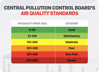
AQI is a standardized metric developed to quantify and communicate the severity of ambient air pollution. It aggregates concentrations of key pollutants—such as PM₂.₅, PM₁₀, NO₂, SO₂, CO, and O₃—into a single dimensionless score. According to the United States Environmental Protection Agency (US EPA), AQI values are classified into six categories: good (0-50), satisfactory (51-100), moderate (101-200), poor (201-300), very poor (301-400), and severe (401-500), each corresponding to varying levels of health concern.
AQI for a particular pollutant is calculated using the following equation:
$A Q I=\left(\frac{I_{\text {high }}-I_{\text {low }}}{C_{\text {high }}-C_{\text {low }}}\right)\left(\mathrm{C}-C_{\text {low }}\right)+I_{\text {low }}$ (1)
where, $C$ is the observed concentration of the pollutant, $C_{\text {low}}$ is the breakpoint concentration ($\leq \mathrm{C}$), $C_{\text {high }}$ is the breakpoint concentration ($\geq \mathrm{C}$), $I_{\text {low }}$ is the AQI value corresponding to $C_{\text {low}}$, and $I_{\text {high}}$ is the AQI value corresponding to $C_{\text {high}}$.
3.1 Study area
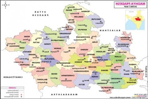
This study focuses on the state of Madhya Pradesh, India. Figure 2 shows all 50 districts, which form the administrative boundaries of Madhya Pradesh. The state is located at the heart of India and is the second-largest state by area and the fifth-largest by population. Having a diverse range of ecological, cultural, and economic landscapes, Madhya Pradesh is an agricultural area, where the substantial proportion of the population is engaged in primary-sector activities, particularly in rural districts. Urban areas, such as the cities of Bhopal, Indore, Jabalpur, and Gwalior, have experienced rapid industrialization and expansion of service-based sectors in recent years.
Figure 2. Districts of Madhya Pradesh, India [31]
3.2 Data collection
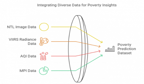
To create a comprehensive dataset for poverty prediction, multiple sources of data were integrated, covering environmental, geospatial and multi-dimensional indicators, as shown in Figure 3.
Figure 3. Integration of various data sources for the poverty prediction model
3.2.1 NTL images
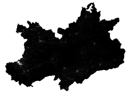
Downloading the NTL images requires the region boundaries. Shapefiles containing boundaries of all districts of Madhya Pradesh for spatial filtering were obtained from the official Geographic Information System (GIS) repository of the state [32]. The shapefile for Ashoknagar District in Madhya Pradesh is shown in Figure 4. The NTL brightness data used in this study was derived from the Visible Infrared Imaging Radiometer Suite (VIIRS) Day/Night Band (DNB) sensor, taken through the Suomi National Polar-orbiting Partnership (Suomi NPP) satellite, operated by the National Oceanic and Atmospheric Administration (NOAA) [33]. The dataset is accessible via Google Earth Engine (GEE). The VIIRS DNB sensor captures radiance values in the 500-900 nm spectral range, offering higher radiometric sensitivity, reduced saturation effects, and finer spatial resolution (~500m per pixel at nadir) compared to its predecessor, DMSP-OLS. The dataset provides daily, monthly, and annual composites, enabling temporal analysis of artificial illumination patterns.
Figure 4. NTL image of Ashoknagar District as a boundary given by the shapefile
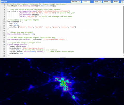
Figure 5. NTL intensity visualization over Bhopal, India, for the year 2023
The VIIRS NTL dataset was chosen due to its high temporal and spatial resolution, improved radiometric sensitivity, and its ability to serve as a proxy for economic activities and electrification. Figure 5 represents the average radiance values in Bhopal, India, for the year 2023 generated using VIIRS DNB data via GEE, with higher light emissions shown in green to red hues, indicating urban and economically active zones. A 10km buffer was applied around the Bhopal region to extract and export the spatial subset.
3.2.2 AQI data
The AQI dataset covers district-level AQI values between 2020 and 2023 from the Madhya Pradesh Pollution Control Board [34], which provides data about air quality trends. AQI is a measure of air pollution that takes into account various pollutants, including particulate matter (PM2.5 and PM10), O3, NO2, and SO2. Higher AQI values correspond to poorer air quality and greater levels of pollution [34]. The AQI dataset was aggregated at the district level, with each data point representing an average AQI score for a specific district and year. The geographic scope includes districts within the state of Madhya Pradesh, India, focusing on regions where poverty is a pressing issue. The temporal range of the dataset spans multiple years, allowing the model to capture changes in air quality over time. This dataset is particularly useful in assessing how changes in environmental quality correlate with economic conditions.
Figure 6. Air quality standards by the Pollution Control Board [35]
To prepare the AQI data for analysis, several pre-processing steps were undertaken:
Step 1: District-level aggregation. AQI values were averaged for each district across each year to smooth out short-term fluctuations and focus on long-term trends.
Step 2: Handling missing data. In districts where AQI data was missing for certain years, imputation techniques were applied and the K-nearest neighbors (KNN) imputation was used to ensure data completeness.
Step 3: Normalization. To ensure compatibility with other datasets, the AQI values were normalized by scaling the data using min-max normalization, bringing all values to a range between 0 and 1.
In this research, the AQI values were treated as a proxy for the economic and industrial development of a district. It is hypothesized that higher levels of pollution, while detrimental to health, may correlate with industrial activities and potentially higher economic outputs, thus influencing poverty levels in unexpected ways. Figure 6 shows the standard values of AQI given by the Pollution Control Board.
3.2.3 VIIRS radiance data
This study used night-time radiance data derived from satellite imagery collected by the VIIRS instrument aboard the Suomi NPP satellite of the National Aeronautics and Space Administration (NASA). The data was obtained via Bhuvan [36], a geoportal developed by the Indian Space Research Organization (ISRO) [37].
The radiance data is spatially disaggregated at the district level, similar to the AQI data. The dataset covers the same time range (2020-2023) and includes all districts within Madhya Pradesh. The spatial resolution of the radiance data is typically around 500 meters, meaning that radiance values are available at a fine granularity, which can be averaged or summed at the district level.
3.2.4 MPI data
This study used MPI data, which is the ground-truth measure for socio-economic conditions given by NITI Aayog [38]. MPI data defines poverty in terms of various aspects to understand the poverty reality of the place. In the MPI framework, headcount ratio and intensity are two critical components that provide insights into the extent and depth of poverty.
Table 1. Categorization of MPI scores and corresponding interpretations
|
Category |
MPI Range |
Interpretation |
|
Non-poor |
0.00-0.099 |
Minimal or no deprivation |
|
Moderately poor |
0.10-0.199 |
Moderate multidimensional poverty |
|
Poor |
0.20 and above |
Severe multidimensional poverty |
• Headcount ratio (H): The proportion of the population that is multidimensionally poor. The headcount ratio measures the percentage of people who are deprived in at least one-third of the weighted indicators of health, education, and standard of living used in MPI. A higher headcount ratio indicates a larger share of the population living in multidimensional poverty.
• Intensity (A): Intensity reflects the severity of poverty, i.e., how deprived poor people are across the multiple indicators. A higher intensity means that poor individuals experience more severe deprivations. As for the relationship between headcount ratio and intensity, MPI is calculated as MPI=H×A. The threshold for poverty classification is 33.33% deprivation by NITI Aayog, equivalent to an MPI score of around 0.10-0.15. Table 1 gives MPI scores and corresponding interpretations. The thresholds are used to classify regions into non-poor, moderately poor, and poor categories based on the extent of multidimensional deprivation experienced.
This section outlines the proposed multimodal approach for poverty prediction, which combines DL-based image feature extraction with environmental indicators (AQI and radiance). The proposed methodology is modular, consisting of three steps: (a) deep feature extraction from satellite imagery, (b) integration of environmental features, and (c) model training and evaluation. Each component is described in detail in the subsequent subsections. A detailed description of the datasets used, including their sources and structure, is provided in the preceding section to establish the understanding of inputs for the model.
4.1 Deep feature extraction
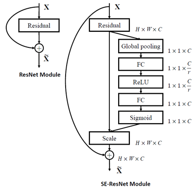
In order to extract deep features from the images, SENet-154 was employed [39]. The SENet-154 architecture, as shown in Figure 7, was developed by integrating Squeeze-and-Excitation (SE) blocks into a modified version of the 64×4d ResNeXt-152 backbone, which extends the ResNeXt-101 design by adopting the block stacking configuration of ResNet-152. First, the number of channels in the initial 1×1 convolution within each bottleneck block was halved to reduce the computational cost with minimal accuracy degradation. Second, the standard 7×7 convolutional layer at the network input was replaced by three consecutive 3×3 convolutions to facilitate better spatial feature extraction. Third, to preserve more informative features during down-sampling, the traditional stride-2 1×1 projection was substituted with a 3×3 stride-2 convolution. District-wise images were resized to 224×224 pixels and normalized. The pre-processed images were passed through the SENet-154 architecture. Features from the last layer were extracted, yielding a 2048-dimensional feature vector for each district.
Figure 7. SENet architecture [39]
4.2 Feature integration
The 2048-dimensional image features extracted from the SENet-154 were combined with two environmental factors: AQI and radiance. AQI and radiance values were standardized using z-score normalization to ensure compatibility with the image features. For each sample, the normalized AQI and radiance values were concatenated with the image feature vector, resulting in a fused 2050-dimensional feature vector (2048+2). This merged data was used to predict poverty labels as per MPI. Algorithm 1 states the steps involved in pre-processing the extracted features from images and merging them with AQI and radiance data.
Algorithm 1. Data pre-processing for multimodal poverty classification
|
Input: -NTL image metadata -AQI, radiance, and MPI datasets Output: - Cleaned and merged feature matrix (X), label vector (y) Start Step 1: Load the datasets Load the NTL image metadata Load AQI, radiance, and MPI datasets Step 2: Handle missing values For each numerical feature x_ij: x_ij=x̄_j if x_ij is missing, else x_ij For each categorical feature: Replace missing values with the most frequent value (mode) Step 3: Encode and normalize Encode the binary poverty label: y_i=1 if 'Poor', else y_i=0 Normalize numerical columns using z-score normalization: x_ij=(x_ij-x̄_j)/σ_j Step 4: Merge data Merge image metadata with AQI, radiance, and MPI datasets using district-year keys End |
4.3 Training model architecture
To integrate AQI and radiance with image-based DL features, this study explored two distinct training approaches for poverty prediction. In the first approach of the baseline SENet-154, features extracted from satellite images using a pretrained SENet-154 model were concatenated with normalized AQI and radiance values after the feature extraction stage. This combined multimodal feature vector was then fed into three ML models, i.e., SVM, RF and XGBoost, for classification. In the second approach of the modified SENet-154, AQI and radiance were directly integrated within the SENet architecture by incorporating AQI and radiance values into the network at the final fully connected (FC) layer for poverty classification. The methodology for each model is outlined step-by-step using algorithmic representations below. Algorithm 2 presents the training workflow for the baseline SENet-154. Algorithm 3 details the modified SENet-154. These structured algorithms highlight the key stages of data pre-processing, feature fusion, and model training for each approach.
Algorithm 2. Baseline SENet-154 with ML classifiers
|
Input: - Pre-processed NTL image dataset for 50 districts for three years - AQI data, radiance data, MPI data Output: - Trained classifiers (SVM, RF, XGBoost) -Poverty labels for districts - Performance metrics Start Step 1: Feature extraction using SENet-154 Load the pre-trained SENet-154 model from the TIMM library Remove the final FC layer Pre-process images: - Resize to 224×224 - Normalize using ImageNet mean and std For each image xi ∈ dataset: Extract 2048-dimensional feature vector: f_img=SENet-154 Step 2: Merge AQI, radiance and MPI data to form a merged dataset Step 3: Train classification algorithms Split the merged dataset into training and testing sets For each classifier Alg_i∈{SVM, RF, XGBoost} do: Initialize Alg_i with chosen parameter 00 Train Alg_i on the training set Step 4: Predict on testing set For each trained classifier Alg_i: Predict labels on the test set: ŷ_i=Alg_i(X_test) Step 5: Evaluate performance metrics Compute the following metrics using ŷ_i and y_test: - Accuracy - Precision - Recall - F1-score Step 6: Select the best model Compare the performance of all models and select the best one End |
Algorithm 3. Modified SENet-154 model
|
Input: - I: Pre-processed NTL image tensor - R: AQI and radiance feature matrix - Y: Binary poverty labels Output: - Trained classification model - Performance metrics on test set Start Step 1: Load and modify SENet-154 Load the pre-trained SENet-154 model from the TIMM library Remove the final FC layer: SENet-154.fc ← Identity () Add a parallel FC layer for auxiliary inputs: Define FC_aux: ℝ² → ℝ²⁰⁴⁸ with ReLU activation Step 2: Feature extraction and fusion For each image xi∈I: Extract deep features: f_img=SENet-154(xi)∈ℝ²⁰⁴⁸ For each auxiliary vector ri ∈R: Transform with auxiliary FC layer: f_aux=ReLU(FC_aux(ri)) ∈ℝ²⁰⁴⁸ Fuse features: f_combined=f_img+f_aux∈ℝ²⁰⁴⁸ Step 3: Classification layer Pass f_combined through a ReLU-activated FC layer: f'=ReLU(W f_combined+b) Apply Softmax/Logits to obtain predictions: ŷ=Softmax(W_final f'+b_final) Step 4: Train the model Initialize the optimizer (Adam) and loss function (CrossEntropy) For each epoch e∈{1, 2, ..., E}: Perform forward pass on training data Compute training loss: ℒ=CrossEntropy(ŷ, Y_true) Backpropagate the gradients Update model weights Log loss and accuracy End for Step 5: Evaluate the model Predict labels on the test dataset Calculate evaluation metrics: accuracy, precision, recall, F1-score End |
A 2050-dimensional feature vector that integrates image features and environmental attributes was created. This dense layer can project the 2050-dimensional input to a 512-dimensional latent space. A final linear layer mapping was performed to a two-dimensional output space corresponding to the binary poverty classification labels (poor/non-poor).
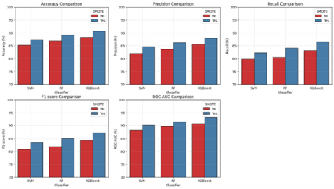
Performance evaluation of models was conducted using ML metrics and spatial validation techniques. Table 2 gives the results by the baseline model in terms of accuracy, precision, recall, F1-score, and Receiver Operating Characteristic-Area Under the Curve (ROC-AUC). As “poor” was the minority class in the dataset, in order to address this class imbalance, Synthetic Minority Over-sampling Technique (SMOTE) [40] was applied during the training phase. SMOTE generates synthetic samples for the minority class which prevents model bias towards the majority class, helping in better generalization across both classes. After applying SMOTE, the models exhibited improved performance metrics, particularly in terms of recall and F1-score for the minority class. The use of SMOTE thus ensured a more balanced training dataset, contributing to more equitable and robust poverty classification outcomes.
Table 2. Performance of the baseline SENet-154 model with and without SMOTE
|
Classifier |
Accuracy (%) |
Precision (%) |
Recall (%) |
F1-Score (%) |
ROC-AUC (%) |
|
SVM |
85.20 |
82.10 |
79.80 |
80.90 |
88.30 |
|
SMOTE SVM |
87.40 |
84.60 |
82.30 |
83.40 |
90.20 |
|
RF |
86.90 |
83.70 |
80.50 |
81.90 |
89.70 |
|
SMOTE RF |
89.10 |
86.20 |
84.10 |
85.10 |
91.50 |
|
XGBoost |
88.30 |
85.50 |
83.20 |
84.30 |
90.80 |
|
SMOTE XGBoost |
90.70 |
88.00 |
86.50 |
87.20 |
93.10 |
Table 3. Performance of the modified SENet-154 model with and without SMOTE
|
Classifier |
Accuracy (%) |
Precision (%) |
Recall (%) |
F1-Score (%) |
ROC-AUC (%) |
|
SVM |
88.10 |
85.30 |
83.10 |
84.20 |
91.20 |
|
SMOTE SVM |
90.40 |
87.60 |
85.90 |
86.70 |
93.50 |
|
RF |
89.80 |
86.90 |
84.70 |
85.80 |
92.10 |
|
SMOTE RF |
92.10 |
89.50 |
87.60 |
88.50 |
94.80 |
|
XGBoost |
91.20 |
88.70 |
86.90 |
87.80 |
93.90 |
|
SMOTE XGBoost |
93.60 |
91.10 |
89.40 |
90.20 |
96.10 |
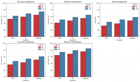
Figure 8 shows the performance comparison histograms of SVM, RF, and XGBoost classifiers with and without SMOTE application. The results demonstrate consistent performance improvements with SMOTE for the minority class. Table 3 shows the performance of the modified SENet-154 model with and without SMOTE. Figure 9 shows the performance comparison histograms of SVM, RF, and XGBoost classifiers with and without SMOTE application for the modified SeNet model across five evaluation metrics.
Figure 8. Performance comparison of SVM, RF, and XGBoost classifiers with and without SMOTE
Figure 9. Performance comparison of SVM, RF, and XGBoost classifiers with and without SMOTE application
5.1 Comparative analysis of the baseline and proposed modified models
Tables 4 and 5 show the differences between the baseline model and the modified SENet-154 model.
Table 4. Baseline SENet-154 model
|
Classifier |
SMOTE |
Accuracy (%) |
Precision (%) |
Recall (%) |
F1-Score (%) |
ROC-AUC (%) |
|
SVM |
Yes |
87.40 |
84.60 |
82.30 |
83.40 |
90.20 |
|
RF |
Yes |
89.10 |
86.20 |
84.10 |
85.10 |
91.50 |
|
XGBoost |
Yes |
90.70 |
88.00 |
86.50 |
87.20 |
93.10 |
Table 5. Modified SENet-154
|
Classifier |
SMOTE |
Accuracy (%) |
Precision (%) |
Recall (%) |
F1-Score (%) |
ROC-AUC (%) |
|
SVM |
Yes |
90.40 |
87.60 |
85.90 |
86.70 |
93.50 |
|
RF |
Yes |
92.10 |
89.50 |
87.60 |
88.50 |
94.80 |
|
XGBoost |
Yes |
93.60 |
91.10 |
89.40 |
90.20 |
96.10 |
Figure 10 shows the performance comparison of the baseline SENet154 model and the modified SENet-154 model with SMOTE application across five evaluation metrics. To validate the observed performance improvements of the proposed model, paired t-tests [41] were conducted on results from 5-fold cross-validation, comparing the baseline and modified models. The modified model consistently outperformed the baseline model across all key metrics. The improvement in accuracy was statistically significant (t(4)=4.32, p=0.012), with a large effect size (Cohen’s d=1.93). Similarly, the F1-score showed a significant increase (t(4)=3.85, p=0.018, d=1.72), and the AUC also improved (t(4)=5.12, p=0.007, d=2.29). These results confirm that integrating environmental variables directly within the feature learning framework can statistically improve the model performance. Table 6 shows the statistical significance testing between models.
Figure 10. Performance comparison of the baseline SENet-154 model and the modified SENet-154 model with SMOTE
Table 6. Comparison of the baseline and modified models with statistical significance testing
|
Metric |
Baseline (Mean±SD) |
Modified (Mean±SD) |
Mean Δ (%) |
T (4) |
P-Value |
Cohen’s D |
|
Accuracy |
0.782±0.028 |
0.840±0.024 |
+5.8 |
4.32 |
0.012 |
1.93 |
|
F1-score |
0.750±0.032 |
0.812±0.027 |
+6.2 |
3.85 |
0.018 |
1.72 |
|
AUC |
0.800±0.025 |
0.865±0.022 |
+6.5 |
5.12 |
0.007 |
2.29 |
5.2 Spatial analysis
To further validate this study, spatial clustering techniques were applied to analyze the geographic distribution of poverty levels. The LISA hotspot analysis [42] was applied, which refers to the use of LISA to detect localized patterns of spatial clustering in geographic data. It identifies hotspots (clusters of high values), cold spots (clusters of low values), and spatial outliers (locations whose values are quite different from their neighbors). The LISA analysis was applied to the MPI scores given by the government and the Predicted Poverty Index (PPI), which were calculated by the proposed model. Algorithm 4 gives an outline of the LISA hotspot analysis.
Algorithm 4. LISA hotspot analysis for poverty
|
Input: - x[1 ... N]: PPI values for N spatial units (districts) - W[N][N]: Spatial weights matrix (e.g., adjacency: 1 if neighbor, 0 otherwise) Output: - Local Moran’s I value for each district - Cluster type for each district: high-high, low-low, high-low, low-high, or not significant Begin: 1. Compute global mean poverty value: mean_x←(1/N)*SUM(x[i] for i=1 to N) 2. Compute standard deviation of poverty: std_x←sqrt ( SUM((x[i]-mean_x)^2)/(N-1)) 3. for each district i=1 to N: a. Initialize local_moran_i ←0 b. For each neighbor j=1 to N: local_moran_i ← local_moran_i+W[i][j]*(x[j]-mean_x) c. Standardize: z_i ← (x[i]-mean_x)/std_x LISA[i] ← z_i*local_moran_i 4. Perform significance test (e.g., permutation test) for each LISA [i] - If p-value < threshold (e.g., 0.05), mark as significant - Else, mark as not significant 5. Determine cluster type: If significant: If z_i>0 and local_moran_i>0→ClusterType[i]←'High-High' If z_i<0 and local_moran_i<0→ClusterType[i]←'Low-Low' If z_i>0 and local_moran_i<0→ClusterType[i]←'High-Low' If z_i<0 and local_moran_i>0→ClusterType[i]←'Low-High' Else: ClusterType[i]←'Not Significant' 6. Output LISA[i] and ClusterType[i] for each district End |
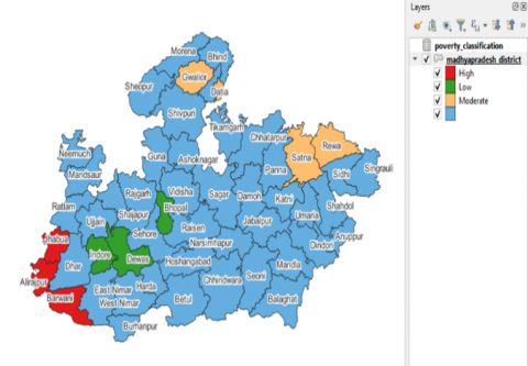
5.2.1 District-level LISA cluster interpretation using MPI
The districts were categorized into high-, moderate-, and low-poverty clusters based on their spatial characteristics by MPI values:
• High-poverty clusters (red): Jhabua, Alirajpur, and Barwani
• Moderate-poverty clusters (yellow): Gwalior, Satna, and Rewa
• Low-poverty clusters (green): Indore, Bhopal, and Dewas
As shown in Figure 11, the remaining districts in blue are baseline areas not classified under the selected thresholds.
Figure 11. District-wise poverty classification map of Madhya Pradesh based on MPI values, generated using QGIS
Table 7. LISA statistics and cluster types for selected Madhya Pradesh districts
|
District |
PPI |
Local Moran's I |
Z-Score |
P-Value |
Cluster Type |
|
Shajapur |
0.058 |
0.557 |
1.627 |
0.104 |
Not significant |
|
Rajgarh |
0.107 |
-0.197 |
-1.856 |
0.064 |
Not significant |
|
Ujjain |
0.061 |
0.614 |
2.095 |
0.036 |
Low-low |
|
Sehore |
0.049 |
0.826 |
2.125 |
0.034 |
Low-low |
|
Dewas |
0.054 |
0.971 |
2.533 |
0.011 |
Low-low |
|
Dhar |
0.077 |
-0.32 |
-1.925 |
0.054 |
Not significant |
|
Alirajpur |
0.192 |
3.234 |
2.754 |
0.006 |
High-high |
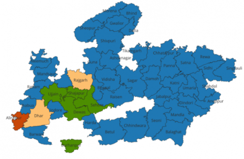
Figure 12. District-wise poverty classification map of Madhya Pradesh based on PPI values, generated using QGIS
5.2.2 District-level LISA cluster interpretation using PPI
The LISA analysis based on PPI scores revealed key spatial poverty patterns across districts in Madhya Pradesh, as shown in Figure 12. A single significant high-high cluster was identified in Alirajpur, indicating a spatial poverty hotspot, similar to the cluster analysis done by MPI. In contrast, five districts, including Dewas, Ujjain, and Sehore, were classified as low-low clusters, representing cold spots of poverty surrounded by similarly low-poverty regions.
Local Moran’s I values for each district were computed to detect spatial autocorrelation in predicted PPI scores. Each district’s result was evaluated for statistical significance by permutation testing (999 permutations). Districts with p-values less than 0.05 were labeled as spatially significant clusters and assigned cluster types, as shown in Table 7.
District-level cluster interpretations were performed on the basis of these values as follows:
Hotspots: Alirajpur
Cold spots (low-low clusters): Dewas, Sehore, and Ujjain
These districts show statistically significant low poverty clusters:
The proposed modified SENet-154 (NTL + AQI + radiance) with the XGBoost classifier outperforms all other models, achieving an accuracy of 93.6%. NTL brightness features remain the strongest predictor but the AQI and radiance integration in the last layer significantly enhance prediction accuracy. With the spatial analysis, it was found that high-poverty clusters, namely Jhabua, Alirajpur, and Barwani, are characterized by low NTL intensity, elevated AQI values, and MPI scores exceeding 0.6, indicating severe deprivation and limited infrastructural development. Moderate poverty regions such as Gwalior, Satna, and Rewa exhibit medium NTL intensity, with AQI values averaging around 100, reflecting an intermediate socio-environmental profile with moderate access to services and infrastructure. Low-poverty districts, including Indore, Bhopal, and Dewas, are associated with high NTL emissions, low MPI values, and relatively cleaner air quality, suggesting better economic conditions and urban infrastructure. These patterns highlight the strong correlation between RS indicators and multidimensional poverty, supporting the utility of integrated geospatial-environmental frameworks for localized poverty assessment.
While the result shows the potential of combining environmental and deep image features for poverty prediction, the method has some limitations. First, MPI, used for comparison of results, was derived from survey data that was reported by the government. Therefore, the data may contain reporting errors that result in biases. In addition, sampling differences could affect how model performance is interpreted. Second, the deep features extracted from the NTL satellite imagery using SENet-154 depend on the image quality of satellite images such as cloud cover, temporal variation, and sensor quality, which impacts feature consistency. Lastly, the environmental features (AQI and radiance) were aggregated at the district level and, in some cases, approximated, limiting the model’s ability to capture minute spatial disparities in poverty conditions.
This study demonstrates the effectiveness of integrating the satellite-based NTL imagery with environmental and socio-economic indicators, specifically AQI and MPI for district-level poverty classification in Madhya Pradesh. The use of DL architectures for feature extraction from NTL data, combined with ML classifiers (SVM, RF, and XGBoost), helped to find out spatial poverty patterns. The application of SMOTE helped in addressing class imbalance and further improved classification performance across key metrics. The results highlight clear segregations, with high-poverty clusters residing in low radiance, poor air quality, and elevated MPI scores. In contrast, districts with high radiance and lower AQI levels were classified as low-poverty zones. The proposed integrated framework not only improves prediction accuracy but also offers actionable insights for policymakers, supporting the formulation of targeted and environmentally informed poverty alleviation strategies. The approach highlights how regional development planning and SDG monitoring at the sub-national level may be strengthened by integrating RS, environmental monitoring, and AI-driven analytics.
Future research could focus on multiple factors associated with this study. First, the integration of additional environmental variables such as land surface temperature, vegetation indices (NDVI), water availability, and noise pollution metrics could provide a better representation of environmental stress factors influencing poverty. Second, incorporating higher-resolution satellite imagery from Sentinel-2, etc., along with socio-demographic census data could further refine poverty prediction at the district level. Employing advanced modeling approaches, including ensemble DL models, graph neural networks (GNNs), or transformer-based architectures, could enhance prediction accuracy by better capturing spatial dependencies. Third, the framework could be extended to other states for analysis, enabling comparative poverty assessments and spatial prioritization for resource allocation. Real-time integration of pollution monitoring and disaster risk indices could make the model more dynamic, assisting policymakers in adaptive planning. Lastly, closer collaboration with governmental agencies could facilitate validation against the ground-truth survey data, enhancing the reliability of the RS-based poverty mapping for practical policy making.
[1] United Nations. (2023). Transforming our world: The 2030 agenda for sustainable development. https://sdgs.un.org/2030agenda, accessed on Apr. 9, 2025.
[2] World Bank. (2023). Chapter 5 Methodology of publication Purchasing power parities and the size of world economies: Results from the 2017 international comparison program. ICP 2017 Global Report: Chapter 5 Methodology. https://thedocs.worldbank.org/en/doc/81d101caf4b3d49bee4b662e5d3ff770-0050022023/, accessed on Apr. 9, 2025.
[3] UNDP & OPHI. (2023). 2023 global multidimensional poverty index (MPI). https://hdr.undp.org/content/2023-global-multidimensional-poverty-index-mpi, accessed on Apr. 15, 2025.
[4] Usmanova, A., Aziz, A., Rakhmonov, D., Osamy, W. (2022). Utilities of artificial intelligence in poverty prediction: A review. Sustainability, 14(21): 14238. https://doi.org/10.3390/su142114238
[5] Srishti Gulecha, R., Muthu Reshmi, K., Rishitha, N., Vani, K. (2024). Poverty mapping in India using machine learning and deep learning techniques. ISPRS Annals of the Photogrammetry, Remote Sensing and Spatial Information Sciences, 10: 319-326. https://doi.org/10.5194/isprs-annals-X-4-2024-319-2024
[6] Addison, D.M., Stewart, B. (2015). Nighttime lights revisited: The use of nighttime lights data as a proxy for economic variables. World Bank Policy Research Working Paper, 7496.
[7] Woodward, H., Oxley, T., Holland, M., Mehlig, D., ApSimon, H. (2024). Assessing PM2.5 exposure bias towards deprived areas in England using a new indicator. Environmental Advances, 16: 100529. https://doi.org/10.1016/j.envadv.2024.100529
[8] Chen, X., Nordhaus, W.D. (2011). Using luminosity data as a proxy for economic statistics. Proceedings of the National Academy of Sciences, 108(21): 8589-8594. https://doi.org/10.1073/pnas.1017031108
[9] Sedda, L., Tatem, A.J., Morley, D.W., Atkinson, P.M., Wardrop, N.A., Pezzulo, C., Sorichetta, A., Kuleszo, J., Rogers, D.J. (2015). Poverty, health and satellite-derived vegetation indices: Their inter-spatial relationship in West Africa. International Health, 7(2): 99-106. https://doi.org/10.1093/inthealth/ihv005
[10] Croft, T.A. (1973). Burning waste gas in oil fields. Nature, 245(5425): 375-376. https://doi.org/10.1038/245375a0
[11] Elvidge, C.D., Baugh, K.E., Kihn, E.A., Kroehl, H.W., Davis, E.R. (1997). Mapping city lights with nighttime data from the DMSP operational linescan system. Photogrammetric Engineering and Remote Sensing, 63(6): 727-734.
[12] Earth Observation Group (EOG). DMSP & VIIRS data download. https://www.ngdc.noaa.gov/eog/download.html, accessed on Sep. 9, 2022.
[13] Mines, C.S.O. Download VIIRS and DMSP products. https://payneinstitute.mines.edu/eog/, accessed on Sep. 9, 2022.
[14] GEE. Google Earth Engine: Data Catalog. https://developers.google.com/earth-engine/datasets/catalog, accessed on Sep. 9, 2022.
[15] Huang, Q., Yang, X., Gao, B., Yang, Y., Zhao, Y. (2014). Application of DMSP/OLS nighttime light images: A meta-analysis and a systematic literature review. Remote Sensing, 6(8): 6844-6866. https://doi.org/10.3390/rs6086844
[16] Jean, N., Burke, M., Xie, M., Alampay Davis, W.M., Lobell, D.B., Ermon, S. (2016). Combining satellite imagery and machine learning to predict poverty. Science, 353(6301): 790-794. https://doi.org/10.1126/science.aaf7894
[17] Ni, Y., Li, X., Ye, Y., Li, Y., Li, C., Chu, D. (2020). An investigation on deep learning approaches to combining nighttime and daytime satellite imagery for poverty prediction. IEEE Geoscience and Remote Sensing Letters, 18(9): 1545-1549. https://doi.org/10.1109/LGRS.2020.3006019
[18] Castro, D.A., Álvarez, M.A. (2023). Predicting socioeconomic indicators using transfer learning on imagery data: An application in Brazil. GeoJournal, 88(1): 1081-1102. https://doi.org/10.1007/s10708-022-10618-3
[19] Ayush, K., Uzkent, B., Tanmay, K., Burke, M., Lobell, D., Ermon, S. (2021). Efficient poverty mapping from high resolution remote sensing images. In Proceedings of the AAAI Conference on Artificial Intelligence, 35(1): 12-20. https://doi.org/10.1609/aaai.v35i1.16072
[20] Yeh, C., Perez, A., Driscoll, A., Azzari, G., Tang, Z., Lobell, D., Ermon, S., Burke, M. (2020). Using publicly available satellite imagery and deep learning to understand economic well-being in Africa. Nature Communications, 11(1): 2583. https://doi.org/10.1038/s41467-020-16185-w
[21] Saeed, S., Turkoglu, I. (2023). Poverty prediction by using deep learning on satellite images. International Journal of Computer Science and Information Technology Research, 11(1): 79-90. https://doi.org/10.5281/zenodo.7766761
[22] Yin, J., Qiu, Y., Zhang, B. (2020). Identification of poverty areas by remote sensing and machine learning: A case study in Guizhou, Southwest China. ISPRS International Journal of Geo-Information, 10(1): 11. https://doi.org/10.3390/ijgi10010011
[23] Lamichhane, B.R., Isnan, M., Horanont, T. (2025). Exploring machine learning trends in poverty mapping: A review and meta-analysis. Science of Remote Sensing, 100200. https://doi.org/10.1016/j.srs.2025.100200
[24] Zheng, X., Zhang, W., Deng, H., Zhang, H. (2024). County-Level poverty evaluation using machine learning, nighttime light, and geospatial data. Remote Sensing, 16(6): 962. https://doi.org/10.3390/rs16060962
[25] Mohale, V.Z., Obagbuwa, I.C. (2024). Poverty analysis and prediction in South Africa using remotely sensed data. Applied Computational Intelligence and Soft Computing, 2024(1): 5137110. https://doi.org/10.1155/2024/5137110
[26] Evans, G.W., Kantrowitz, E. (2002). Socioeconomic status and health: The potential role of environmental risk exposure. Annual Review of Public Health, 23(1): 303-331. https://doi.org/10.1146/annurev.publhealth.23.112001.112349
[27] Rentschler, J., Leonova, N. (2023). Global air pollution exposure and poverty. Nature Communications, 14(1): 4432. https://doi.org/10.1038/s41467-023-39797-4
[28] Magesh, S., Geng, K. (2025). A machine learning interpretation of the correlation between poverty and air pollution in the contiguous United States. Scientific Reports, 15(1): 2407. https://doi.org/10.1038/s41598-025-87150-0
[29] Clark, L.P., Millet, D.B., Marshall, J.D. (2014). National patterns in environmental injustice and inequality: Outdoor NO2 air pollution in the United States. PLoS ONE, 9(4): e94431. https://doi.org/10.1371/journal.pone.0094431
[30] Centre for Science and Environment. Delhi air pollution hits severe levels, schools shut down. https://www.cseindia.org, accessed on Sep. 9, 2022.
[31] MapsofIndia. District Map of Madhya Pradesh. https://www.mapsofindia.com, accessed on Jan. 25, 2025.
[32] Madhya Pradesh Geoportal. Our projects. https://www.geoportal.mp.gov.in/geoportal/OurProjects.aspx, accessed on Jan. 22, 2025.
[33] Elvidge, C.D., Zhizhin, M., Ghosh, T., Hsu, F.C., Taneja, J. (2021). Annual time series of global VIIRS nighttime lights derived from monthly averages: 2012 to 2019. Remote Sensing, 13(5): 922. https://doi.org/10.3390/rs13050922
[34] MPPCB. Environmental monitoring data: AQI. https://erc.mp.gov.in/EnvAlert/AQI, accessed on Jan. 24, 2025.
[35] MPPCB. Ambient air quality of Madhya Pradesh. https://www.mppcb.mp.gov.in/Ambient-Air-Quality-of-MP-22.aspx, accessed on Dec. 24, 2024.
[36] Central Pollution Control Board (CPCB). (2024). National air quality index. Ministry of Environment, Forest and Climate Change, Government of India. https://cpcb.nic.in/National-Air-Quality-Index/, accessed on Apr. 1, 2025
[37] ISRO Bhuvan Portal: Nighttime Light Data. https://bhuvan-app1.nrsc.gov.in/bhuvan_ntl/, accessed on Nov. 8, 2024.
[38] NITI Aayog. (2023). India national multidimensional poverty index (A progress review 2023). https://www.niti.gov.in/sites/default/files/2023-08/India-National-Multidimentional-Poverty-Index-2023.pdf, accessed on Jan. 1, 2025.
[39] Hu, J., Shen, L., Sun, G. (2018). Squeeze-and-excitation networks. In Proceedings of the IEEE Conference on Computer Vision and Pattern Recognition, Salt Lake City, UT, USA, pp. 7132-7141. https://doi.org/10.1109/CVPR.2018.00745
[40] Chawla, N.V., Bowyer, K.W., Hall, L.O., Kegelmeyer, W.P. (2002). SMOTE: Synthetic minority over-sampling technique. Journal of Artificial Intelligence Research, 16: 321-357. https://doi.org/10.1613/jair.953
[41] Ruxton, G.D. (2006). The unequal variance t-test is an underused alternative to student's t-test and the Mann-Whitney U test. Behavioral Ecology, 17(4): 688-690. https://doi.org/10.1093/beheco/ark016
[42] Anselin, L. (1995). Local indicators of spatial association-LISA. Geographical Analysis, 27(2): 93-115. https://doi.org/10.1111/j.1538-4632.1995.tb00338.x