Firdaous Khemlichi*![]() | Youness Idrissi Khamlichi
| Youness Idrissi Khamlichi![]() | Safae Elhaj Ben Ali
| Safae Elhaj Ben Ali![]()
© 2025 The authors. This article is published by IIETA and is licensed under the CC BY 4.0 license (http://creativecommons.org/licenses/by/4.0/).
OPEN ACCESS
Financial markets are highly dynamic, driven by complex interactions between sentiment, volatility, and structural asset dependencies. Traditional portfolio optimization methods often rely on static assumptions, rendering them ineffective under volatile or rapidly shifting conditions. To address these limitations, we propose a Modular Portfolio Learning System (MPLS) based on a hierarchical multi-agent reinforcement learning architecture. MPLS dynamically adjusts asset allocations in response to multi-source market signals, guided by a central Decision Fusion Framework (DFF) trained via Proximal Policy Optimization (PPO). The system integrates three analytical modules: (1) a Sentiment Analysis Module (SAM) leveraging FinBERT to extract market mood from financial news, (2) a Volatility Forecasting Module (VFM) combining LSTM and Bayesian modeling for risk estimation, (3) a Graph Neural Network (GNN) that captures inter-asset and sectoral relationships. A dedicated PPO agent in DFF learns to adaptively fuse these signals over time. The hierarchical architecture of MPLS features a High-Level Agent (HLA) for sector allocation and Low-Level Agents (LLAs) for intra-sector decisions, combining strategic foresight with tactical flexibility. Empirical results across S&P 500, DAX, and FTSE 100 under multiple regimes show that MPLS outperforms conventional baselines, achieving up to +38.2% improvement in Sharpe Ratio and −24.1% reduction in maximum drawdown compared to single-agent PPO and risk-parity models. MPLS thus provides a scalable and interpretable solution for adaptive portfolio optimization under uncertainty.
portfolio optimization, reinforcement learning, multi-agent systems, financial times series forecasting, sentiment analysis, graph neural networks, volatility forecasting
Financial markets are complex and highly dynamic, influenced by macroeconomic factors, investor sentiment, volatility fluctuations, and inter-sector dependencies [1-4]. Traditional portfolio optimization techniques, such as Markowitz’s mean-variance model [5], rely on static assumptions and often fail to capture abrupt market regime shifts. Although machine learning [6] and reinforcement learning (RL) [7] approaches have shown promise in adapting to changing environments, they frequently operate in isolation, lacking integration of diverse market signals into a unified decision-making framework.
To address these challenges, we propose the Modular Portfolio Learning System (MPLS)—a hierarchical multi-agent reinforcement learning framework [8] designed to optimize portfolio allocations dynamically. MPLS integrates sentiment analysis, volatility forecasting, and inter-asset dependency modeling into a unified learning architecture, enabling it to continuously adjust strategies in response to evolving market conditions. By jointly leveraging behavioral, statistical, and structural signals, MPLS captures a more holistic representation of the market, enhancing its adaptability and robustness.
To learn optimal decision policies, MPLS employs Proximal Policy Optimization (PPO) [9], a policy-gradient reinforcement learning algorithm known for its training stability and sample efficiency. This enables the system to balance return maximization with dynamic risk control, offering a robust solution to modern portfolio management.
This paper presents the following key contributions to portfolio optimization research:
The remainder of this paper is organized as follows: Section 2 reviews related work in portfolio optimization and reinforcement learning. Section 3 presents the MPLS framework, detailing its architecture, analytical components, and reinforcement learning mechanisms. Section 4 describes the experimental setup, including datasets, preprocessing, and evaluation metrics. Section 5 discusses the results and ablation studies, and Section 6 concludes the paper and outlines potential directions for future research.
Portfolio optimization has traditionally relied on statistical models such as the Markowitz mean-variance framework. While foundational, these approaches assume linearity and stationarity, making them ineffective in volatile or non-stationary markets. To address these limitations, recent research has turned to deep reinforcement learning (DRL) [13-15] with algorithms like Deep Q-Network [16-18], Deep Deterministic Policy Gradient [19], and PPO [9] showing promise in learning adaptive trading policies from historical data [20, 21].
Multi-agent reinforcement learning (MARL) has also emerged to decompose complex decision-making tasks. Hierarchical MARL, such as FeUdal Networks [8], improves scalability and interpretability by separating high-level strategy from low-level execution [8]. However, these approaches are rarely applied to real-world portfolio systems or fail to integrate diverse financial signals in a unified manner.
Recent advances in reinforcement learning have introduced transformer-based models that leverage temporal self-attention to capture long-range market dependencies [22, 23]. While these architectures have achieved strong empirical results in financial tasks, their deployment remains limited by high computational demands and reduced interpretability. In parallel, hierarchical reinforcement learning (HRL) methods—such as option-critic and HRL-PPO variants [24], —have been explored to model temporally abstract decision layers, improving sample efficiency and policy stability in long-horizon settings. However, these approaches are often evaluated in synthetic environments or focus on narrow signal types. To the best of our knowledge, existing methods rarely offer a unified, modular architecture that integrates diverse sources such as sentiment, volatility, and structural interdependencies in a manner tailored to real-world portfolio optimization.
Complementary techniques have focused on modeling individual signals. FinBERT [10] has been used to extract sentiment from financial news, while LSTM-based models address volatility forecasting [11]. Graph Neural Networks (GNNs), particularly Graph Attention Networks (GATs), are increasingly used to model asset interdependencies, though most applications focus on prediction rather than allocation and seldom integrate with RL frameworks [25].
In contrast, the MPLS integrates hierarchical reinforcement learning with dynamic signal fusion across sentiment, volatility, and structural dependencies. This unified and interpretable framework addresses the fragmentation of prior work and supports robust, adaptive portfolio optimization under uncertainty.
3.1 MPLS architecture
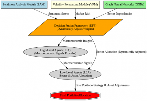
The MPLS is a hierarchical multi-agent reinforcement learning framework for adaptive portfolio optimization. It responds to evolving market dynamics by fusing sentiment, volatility, and structural signals within a unified learning architecture. An overview of the system’s architecture is illustrated in Figure 1.
Figure 1. The decision flow in the MPLS framework
MPLS features a two-tier agent hierarchy: An HLA sets sector-level strategies based on macroeconomic trends, sentiment, and volatility forecasts, while sector-specific LLAs refine asset-level allocations using localized indicators. This separation of strategic and tactical control enhances flexibility and scalability.
To capture interdependencies across assets and sectors, MPLS incorporates GNNs, modeling the market as a dynamic graph of financial relationships. Each agent learns policies within a Markov Decision Process (MDP), and final decisions are coordinated via a Decision Fusion Framework (DFF) that adaptively weights signal contributions using reinforcement learning.
3.2 SAM
The SAM plays a pivotal role in the MPLS by transforming unstructured financial text into actionable sentiment signals. Given that investor sentiment often drives short-term market dynamics and volatility [2], SAM provides a quantifiable measure of market mood, enabling MPLS to incorporate behavioral finance insights into its portfolio decision-making process.
SAM processes financial news, analyst reports, earnings call transcripts, and social media using FinBERT [10], a transformer model specifically fine-tuned on financial text corpora.
For each document d, the sentiment score $s_d$ is computed as:
$S_d=\left[p_{{pos }}, p_{ {neu }}, p_{ {neg }}\right]$ (1)
where, ppos, pneu, and pneg represent the predicted probabilities of positive, neutral, and negative sentiment. These values are aggregated across sources and time to form a daily sentiment index [26], adjusted for source credibility and volume using weighted averaging and a 3–5 days exponential smoothing filter.
To align sentiment with trading data, timestamps are matched to trading days. Same-day impact is assumed for news, while social media and earnings calls are lagged by one day to account for delayed reactions.
To mitigate noise and misinformation—especially during crises like COVID-19—SAM incorporates three mechanisms: (i) confidence-based filtering discards low-certainty FinBERT outputs (< 0.6); (ii) sentiment scores are smoothed using a 3-day EMA; (iii) emotionally charged keywords are normalized to reduce overreaction to social media language.
A feedback loop further refines model weights if sentiment predictions contradict actual market behavior. These robustness techniques ensure SAM remains stable and informative even under extreme market narratives.
Given its daily inference structure, SAM operates in batch mode and completes processing within 45 seconds on standard GPU hardware. Its modular implementation supports parallel execution, ensuring low-latency integration with the DFF.
The resulting sentiment index is passed to the Decision Fusion Framework (Section 3.5), where it is combined with other signals for final allocation decisions.
3.3 VFM
The VFM estimates market uncertainty using a hybrid architecture that combines sequential learning with uncertainty modeling. It fuses an LSTM network, which captures temporal patterns in historical volatility and returns, with a Bayesian Network that provides predictive variance estimates. Given an input sequence $X_t$ of past volatility values, the LSTM predicts a mean future volatility:
$\hat{\mu}_t=f_{L S T M}\left(X_t\right)$ (2)
To account for uncertainty, a Bayesian Network outputs the full volatility distribution:
$P\left(\sigma_t^2 \mid X_t, Z_t\right)=N\left(\mu_t, \sigma_t^2\right)$ (3)
In Eq. (3), $Z_t$ denotes a vector of macro-financial indicators used to condition the Bayesian inference process. These include interest rates, inflation, market volatility indices, and sector-level economic signals. Unlike neural embeddings, these features are selected based on domain expertise and data availability, allowing for interpretable modeling of causal financial relationships.
This dual-model approach enables VFM to deliver both precise volatility forecasts and associated confidence intervals. When the estimated uncertainty $\sigma_t^2$ exceeds a predefined threshold, the system promotes a more conservative allocation strategy. This threshold was empirically calibrated by analyzing the distribution of posterior variance estimates over the 2010–2018 training period. The 75th percentile of this distribution was selected to effectively capture abnormal volatility episodes while avoiding excessive reactivity to moderate fluctuations.
Notably, VFM employs a classical Bayesian Network, not a Bayesian Neural Network (BNN). This choice ensures greater interpretability and computational efficiency. The Bayesian structure captures conditional dependencies among macroeconomic inputs, using a hybrid strategy that combines domain knowledge and data-driven structure learning. Key relationships—such as inflation influencing interest rates, and interest rates affecting volatility—are encoded based on macroeconomic theory. In addition, structure learning algorithms (PC and BIC) were applied on historical macro-financial data (2010–2018) to detect latent dependencies. The final graph was selected based on likelihood score to ensure both robustness and interpretability.
VFM’s volatility forecasts and associated confidence bounds are sent to the DFF for downstream fusion and decision-making (see Section 3.5).
3.4 GNN module
The GNN module in MPLS models interdependencies among assets, sectors, and macroeconomic indicators. Unlike traditional methods that assume asset independence, it leverages GATs to learn dynamic financial relationships.
The market is represented as a graph G=(V,E), where nodes $v_i \in V$ denote assets or sectors, and edges $\left(v_i, v_j\right) \in E$ capture co-movement or sectoral links. Node features $h_i$ integrate historical returns, sentiment scores (from SAM), and volatility forecasts (from VFM).
Edge weights are computed using 60-day rolling Pearson correlations, updated every $T_g=5$ trading days. This weekly interval balances responsiveness and noise control, as shorter windows proved unstable and longer ones lagged in adapting to structural shifts.
The GAT architecture comprises four layers, selected empirically for its optimal balance between expressiveness and stability. Deeper configurations (e.g., six layers) led to oversmoothing, degrading performance. To regularize training, dropout (0.2), LeakyReLU activation, and layer normalization are applied.
$h_i^{(t+1)}=\sigma\left(W . \sum_{j \in N(i)} \alpha_{i j} h_j^{(t)}\right)$ (4)
In Eq. (4), $N(i)$ denotes the set of neighbors of node i, and $\alpha_{i j}$ represents the attention coefficient between node i and node j, which is learned during GAT training. This aggregation mechanism allows each node to refine its embedding using the weighted contributions of its neighbors.
Full training configuration of GAT layers is detailed in Section 4.1.
Learned node embeddings are fed into LLAs and the DFF, enriching decisions with structural context. Trained jointly via PPO, the GNN dynamically adapts to evolving market topologies, enabling MPLS to: detect sector momentum and reversals, capture cross-asset influence patterns, adapt to correlation shifts across regimes, and mitigate systemic risk through structural diversification.
3.5 Decision fusion and multi-agent coordination
MPLS adopts a hierarchical multi-agent reinforcement learning architecture powered by PPO. The system coordinates macro-level strategies through an HLA, which allocates capital across sectors, and LLAs, which execute asset-level decisions within each sector. The DFF is implemented as an autonomous PPO-trained agent. Rather than applying fixed or rule-based weightings, it learns a dynamic fusion policy that adjusts the importance of each analytical module (SAM, VFM, GNN) based on evolving market conditions. Its goal is to maximize long-term portfolio performance by learning to emphasize reliable signals and downweight misleading ones. This formulation enables the DFF to serve as a policy-driven aggregator, rather than a static fusion layer.
At each timestep t, the DFF constructs a fusion state vector aggregating signals from the SAM, VFM, and GNN:
$S_{ {fusion }}=\left[S_{{sentiment}}, S_{{volatility }}, S_{G N N}\right]$ (5)
A Softmax layer outputs attention weights:
$A_{{fusion }}=\left[\omega_{ {sentiment }}, \omega_{ {volatility }}, \omega_{G N N}\right], \sum \omega_i=1$ (6)
Each analytical module (SAM, VFM, GNN) proposes its own sector-level allocation vector $a_k$. These vectors are aggregated by the DFF using the attention weights to form a single fused sector allocation:
$\pi(s)=\sum_{k=1}^k \omega_k . a_k$ (7)
This fused policy π(s) is then passed to the HLA, which uses it as a base strategy to allocate capital across sectors. In other words, the HLA does not act independently, but conditions its final sector allocation directly on this weighted fusion output. The resulting sector weights are then passed to LLAs, which refine allocations at the asset level within each sector. LLAs take into account both the high-level sector allocation from the HLA and sector-specific dynamics to ensure responsive and regime-aware execution. This two-tiered delegation ensures both strategic alignment (via DFF and HLA) and tactical adaptability (via LLAs).
Reward Structure and Optimization
The PPO agent in DFF, along with the HLA and LLAs, receives a reward at the end of each episode based on risk-adjusted performance:
$R=\alpha . S R-\beta . \sigma$ (8)
In Eq. (8), the reward signal combines the Sharpe Ratio (SR) and the annualized portfolio volatility (σ). The coefficients α and β govern the trade-off between return maximization and risk penalization. In our initial configuration, we used α=1 and β=0.8, giving slightly more weight to return than to volatility. These initial values were subsequently fine-tuned on the validation set via Bayesian optimization, yielding optimal values of α=1.2 and β=1.0, which provide greater sensitivity to drawdown risk without suppressing performance gains.
State and Action Representations
$S_t^{H L A}=\left[M I_t, G S_t, V F_t, P H_t\right]$ (9)
where, $M I_t, G S_t, V F_t$ and ${PH}_t$ refer to MacroIndicators, GlobalSentiment, VolatilityForecast, and PortfolioHistory, respectively.
$a_t^{H L A}=\left[w_{ {Tech }}, w_{ {Healthcare }}, w_{ {Energy }}\right]$ (10)
$s_t^{L L A}=\left[S S_t, S V_t, A T_t, G R_t\right]$ (11)
where, $S S_t, S V_t, A T_t$ and $G R_t$ refer to Sector Sentiment, Sector Volatility, Asset Trends, and GNN Relations, respectively.
$a_t^{L L A}=\left[w_{A_1}, w_{A_2}, \ldots, w_{A_n}\right]$ (12)
Learning Horizon and Stability
The modular nature of this architecture allows interpretability and scalability. Each module’s outputs (e.g., FinBERT sentiment scores, GNN correlations, and volatility estimates) can be analyzed independently to understand their contribution to final allocation decisions.
4.1 Experimental setup
We evaluate MPLS using a ten-year dataset (2010–2020) that integrates 60 stocks from the S&P 500 (U.S.) [27], DAX (Germany) [28], and FTSE 100 (U.K.) [29] indices. To ensure diversity and avoid selection bias, 20 stocks per index were selected based on liquidity (average daily volume), market capitalization, and sectoral coverage across Technology, Healthcare, and Energy.
The dataset includes OHLCV data, macroeconomic indicators (interest rates, inflation, GDP from Fed, ECB, BoE), volatility indices, and sentiment scores extracted using FinBERT from financial news. All data are synchronized on a unified daily timeline (UTC-based). Regional market discrepancies are addressed by mapping each asset’s closing price to the same calendar day, and non-trading days are handled via forward-filling. To handle non-synchronous trading hours (e.g., between U.S. and European markets), closing prices are normalized to a unified reference day using time zone alignment and latest-available value mapping. Macroeconomic and sentiment data are timestamp-aligned, with a one-day lag when necessary to reflect realistic information availability.
The dataset is split chronologically: 70% for training, 10% for validation, and 20% for testing. Model evaluation relies on standard financial metrics, ensuring fair and consistent performance comparisons across market regimes.
We assess system performance in two distinct market regimes:
Model Architecture and Training Configuration
For reproducibility and clarity, we specify the architectural and training details of each core module. The SAM utilizes FinBERT, initialized with pretrained weights and fine-tuned for five epochs on a financial news corpus using a learning rate of $2 \times 10^{-5}$, a batch size of 32, and the Adam optimizer. The classification head includes two fully connected layers of sizes [768, 128] with ReLU activation.
The VFM comprises a two-layer LSTM with 64 hidden units per layer, using tanh activation and a dropout rate of 0.3. The Bayesian Network contains 10 nodes representing macroeconomic and market indicators, with a hybrid expert/data-driven structure and parameters learned via maximum likelihood estimation.
The GNN module adopts a four-layer GAT, each with 64 hidden units and four attention heads, using LeakyReLU activation and layer normalization.
All PPO-based agents (HLA, LLA, and DFF) are trained using a shared configuration: learning rate $3 \times 10^{-4}$, clip ratio 0.2, entropy coefficient 0.01, and the Adam optimizer. Policy/value networks have hidden layers of sizes [256, 128] with ReLU activation, trained for 10 epochs per update using a mini-batch size of 256 and 2048 rollout steps.
Hyperparameter Tuning
To ensure fair and stable training across all PPO-based agents, we employ a hybrid tuning strategy combining grid search and Bayesian optimization. A Gaussian process-based optimizer with an Expected Improvement acquisition function is used to explore promising regions of the hyperparameter space, following [27].
The final configuration, applied uniformly across the HLA, LLAs, and the DFF, is summarized in Table 1.
Table 1. Hyperparameters used in MPLS training
|
Parameter |
Value |
|
Learning rate |
$3 \times 10^{-4}$ |
|
PPO clip ratio |
0.2 |
|
Entropy coefficient |
0.01 |
|
Discount factor ($\gamma$) |
0.99 |
|
GAE Lambda ($\lambda$) |
0.95 |
|
Value loss coefficient |
0.5 |
|
Update steps |
2048 |
|
Mini-batch size |
256 |
|
PPO epochs |
10 |
|
Optimizer |
Adam |
|
Gradient clipping |
Max norm = 0.5 |
Evaluation Metrics
System performance is measured using the following financial metrics:
Baseline Models for Comparison
To evaluate the added value of the MPLS framework, we benchmark against:
These baselines offer diverse comparisons—traditional, learning-based, and naive—demonstrating the system’s strengths in adaptability, modularity, and risk-aware decision-making.
Computational Infrastructure and Optimization Trials
To support efficient training and reproducibility, all PPO-based agents (HLA, LLA, and DFF) were optimized using Bayesian optimization with Gaussian Processes and the Expected Improvement acquisition function. Each agent type underwent 50 optimization trials, leveraging a 3-fold cross-validation scheme on the training set.
Experiments were conducted on Google Colab Pro+ with an NVIDIA Tesla T4 GPU (16 GB VRAM), 32 GB RAM, and an Intel Xeon 2.2GHz CPU. Each complete training run required approximately 2.5 hours per agent configuration, balancing computational feasibility and search depth.
4.2 Performance evaluation
We assess MPLS against three baselines—Markowitz MVO, Single-Agent RL, and Equal-Weighted Portfolio (EWP)—across two distinct regimes: pre-COVID (stable) and COVID (volatile). MPLS outperforms all baselines on cumulative return, risk-adjusted ratios (Sharpe, Sortino), and drawdown control in both regimes.
All results reported in this section are computed under the assumption of frictionless execution—excluding transaction costs, slippage, and leverage—to maintain consistency and comparability across all evaluated models.
In the pre-COVID phase, MPLS achieved a Sharpe Ratio of 2.31 and a cumulative return of 39.87%, outperforming Single-Agent RL (34.98%) and MVO (27.68%). It also maintained a lower drawdown (−8.46%) and moderate volatility (22.18%).
During COVID, MPLS remained robust despite extreme conditions, reaching a Sharpe Ratio of 2.08, with reduced drawdown (−14.83%) and a cumulative return of 49.75%, outperforming Single-Agent RL (37.64%) and all baselines.
While transaction costs and slippage were not modeled to preserve fair comparisons, their impact is acknowledged. Future extensions will integrate cost-aware components (e.g., liquidity spreads, slippage). To capture tail risk, we also report VaR and CVaR at the 95% confidence level. MPLS consistently exhibited lower values across regimes, confirming its ability to mitigate rare but severe losses (see Tables 2-3).
Table 2. Performance in the pre-COVID period
|
Model |
MPLS |
MVO |
Single Agent |
EWP |
|
Sharpe Ratio |
2.31 |
1.79 |
1.92 |
1.38 |
|
Sortino Ratio |
3.74 |
3.02 |
2.51 |
1.91 |
|
Max Drawdown |
-8.46 |
-12.12 |
-10.23 |
-18.34 |
|
Annual Volatility |
22.18 |
18.03 |
20.17 |
15.06 |
|
Cumulative Return |
39.87% |
27.68% |
34.98% |
17.82% |
|
VaR@95% |
-6.12% |
-7.35% |
-6.85% |
-8.57% |
|
CvaR@95% |
-9.03% |
-10.12% |
-9.45% |
-12.18% |
Table 3. Performance in the COVID period
|
Model |
MPLS |
MVO |
Single Agent |
EWP |
|
Sharpe Ratio |
2.08 |
1.58 |
1.81 |
1.19 |
|
Sortino Ratio |
3.47 |
2.77 |
2.32 |
1.72 |
|
Max Drawdown |
-14.83 |
-20.38 |
-17.65 |
-24.76 |
|
Annual Volatility |
29.92 |
24.86 |
27.89 |
18.11 |
|
Cumulative Return |
49.75% |
21.93% |
37.64% |
10.42% |
|
VaR@95% |
-9.12% |
-10.27% |
-9.84% |
-11.35% |
|
CvaR@95% |
-13.84% |
-15.96% |
-14.52% |
-17.61% |
4.3 Ablation study: Module impact analysis
To evaluate the role of each module in MPLS, we conduct ablation experiments by selectively removing the SAM, the VFM, or the GNN. Performance drops observed across both pre-COVID and COVID regimes (Tables 4-5) confirm that each component contributes meaningfully to risk-adjusted returns and volatility control.
Table 4. Performance without SAM, VFM, GNNs - pre-COVID period
|
Model |
FULL MPLS |
NO SAM |
NO VFM |
NO GNNs |
|
Sharpe Ratio |
2.31 |
2.06 |
1.84 |
1.96 |
|
Sortino Ratio |
3.74 |
3.21 |
2.88 |
2.97 |
|
Max Drawdown |
-8.46% |
-10.47% |
-12.16% |
-11.02% |
|
Annual Volatility |
22.18% |
23.48% |
24.53% |
22.91% |
|
VaR@95% |
-6.12% |
-6.88% |
-7.41% |
-7.19% |
|
CvaR@95% |
-9.03% |
-10.22% |
-11.38% |
-10.71% |
Table 5. Performance without SAM, VFM, GNNs - COVID period
|
Model |
FULL MPLS |
NO SAM |
NO VFM |
NO GNNs |
|
Sharpe Ratio |
2.08 |
1.82 |
1.58 |
1.76 |
|
Sortino Ratio |
3.47 |
2.81 |
2.46 |
2.61 |
|
Max Drawdown |
-14.83% |
-19.87% |
-22.41% |
-21.07% |
|
Annual Volatility |
29.92% |
32.48% |
34.96% |
33.04% |
|
VaR@95% |
-9.12% |
-10.83% |
-12.29% |
-11.64% |
|
CvaR@95% |
-13.84% |
-15.94% |
-17.73% |
-16.42% |
Results from the pre-COVID and COVID periods are presented in Tables 4 and 5, respectively. In the pre-COVID environment, the removal of any individual module leads to a noticeable decline in Sharpe and Sortino Ratios, along with increases in both maximum drawdown and annualized volatility. For instance, excluding VFM results in the most significant performance drop, with a reduction in the Sharpe Ratio from 2.31 to 1.84 and an increase in drawdown from -8.46% to -12.16%. The absence of SAM also degrades performance, though to a lesser extent, highlighting its importance in stable market conditions for capturing investor sentiment trends.
During the pre-COVID period, excluding VFM led to the sharpest degradation (Sharpe: 2.31 → 1.84), while SAM and GNNs also showed measurable but smaller impacts. In the COVID phase, the importance of VFM and GNNs grew, highlighting their role in managing structural risk and uncertainty. SAM’s influence weakened due to erratic sentiment shifts, but still added value under calmer conditions.
To assess inter-module synergy, we further tested combinations of removed modules (e.g., SAM + VFM), with results presented in Tables 6-7. All combinations significantly underperformed the full MPLS. For instance, removing SAM and VFM jointly led to a 42.6% drop in Sharpe Ratio during COVID. Across all ablations, performance degradation was statistically significant (p < 0.01), and VaR/CVaR scores worsened, confirming reduced resilience.
Table 6. Combined module removal – pre-COVID period
|
Model |
FULL MPLS |
NO SAM + VFM |
NO SAM + GNNs |
NO VFM + GNNs |
|
Sharpe ± Std |
2.31 ± 0.06 |
1.63 ± 0.08 |
1.74 ± 0.07 |
1.58 ± 0.10 |
|
Return ± Std |
39.87 ± 1.22 |
29.32 ± 1.84 |
31.18 ± 1.67 |
27.81 ± 2.11 |
|
p-value (vs Full) |
- |
0.004 |
0.006 |
0.002 |
|
VaR@95% |
-6.12% |
-7.92% |
-8.41% |
-9.12% |
|
CvaR@95% |
-9.03% |
-11.96% |
-12.88% |
-13.72% |
Table 7. Combined module removal – COVID period
|
Model |
FULL MPLS |
NO SAM + VFM |
NO SAM + GNNs |
NO VFM + GNNs |
|
Sharpe ± Std |
2.08 ± 0.05 |
1.20 ± 0.09 |
1.38 ± 0.07 |
1.25 ± 0.08 |
|
Return ± Std |
49.75 ± 1.35 |
30.12 ± 2.24 |
33.47 ± 1.94 |
31.02 ± 1.76 |
|
p-value (vs Full) |
- |
0.001 |
0.003 |
0.002 |
|
VaR@95% |
-9.12% |
-12.43% |
-11.95% |
-12.67% |
|
CvaR@95% |
-13.84% |
-17.32% |
-16.52% |
-17.89% |
These results validate the complementary roles of SAM, VFM, and GNNs. While VFM is critical in volatile markets, GNNs contribute consistently by capturing interdependencies, and SAM enhances tactical responsiveness in stable conditions. Their combined integration via DFF is key to the system’s robustness and adaptability.
4.4 Generalization to post-2020 regimes
To assess the robustness of MPLS under more recent and structurally distinct market conditions, we extended the evaluation to include the 2021–2023 period. This timeframe captures the aftermath of COVID-19, characterized by macroeconomic instability including inflation surges, interest rate hikes, and sector rotations.
MPLS maintained strong performance, achieving a Sharpe Ratio of 2.12, a maximum drawdown of −10.71%, and consistently lower tail-risk exposure as measured by VaR and CVaR. These results highlight the model’s adaptability to unseen regimes and reinforce its robustness beyond the original training horizon. Table 8 summarizes the system’s performance metrics over the 2021–2023 period, further confirming its ability to generalize beyond the COVID training window.
Table 8. Performance in the post-COVID period (2021-2023)
|
Model |
MPLS |
MVO |
Single Agent |
EWP |
|
Sharpe Ratio |
2.12 |
1.61 |
1.85 |
1.32 |
|
Sortino Ratio |
3.59 |
2.81 |
2.47 |
1.89 |
|
Max Drawdown |
-10.71% |
-15.20% |
-13.56% |
-21.34% |
|
Annual Volatility |
24.80% |
19.96% |
22.47% |
16.02% |
|
Cumulative Return |
42.13% |
28.45% |
35.72% |
16.89% |
|
VaR@95% |
-8.42% |
-9.03% |
-8.67% |
-9.87% |
|
CvaR@95% |
-12.75% |
-13.81% |
-13.12% |
-14.92% |
4.5 Sector allocation analysis
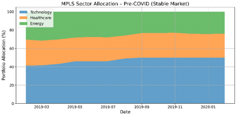
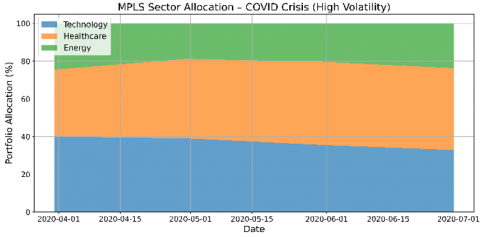
To evaluate the adaptability of the MPLS in adjusting portfolio composition under varying market regimes, we analyze the evolution of sector-level allocations across three core industries: Technology, Healthcare, and Energy. This analysis spans two distinct periods—pre-COVID (stable market) and COVID (high-volatility)—offering insight into how MPLS reallocates capital in response to changing economic signals and investor sentiment as shown in Figure 2.
During the pre-COVID period, MPLS consistently maintains a higher allocation to the Technology sector, reflecting its alignment with growth-oriented market conditions. Allocations to Healthcare and Energy remain comparatively stable, with only moderate fluctuations over time. This behavior illustrates MPLS’s ability to preserve diversification while capitalizing on high-performing sectors during periods of low volatility.
Conversely, in the COVID-19 crisis period, the system demonstrates a pronounced shift in sector allocation. Exposure to Technology is reduced amid increasing uncertainty, while Healthcare allocations rise significantly, signaling a strategic reallocation toward defensive sectors known for stability during macroeconomic shocks.
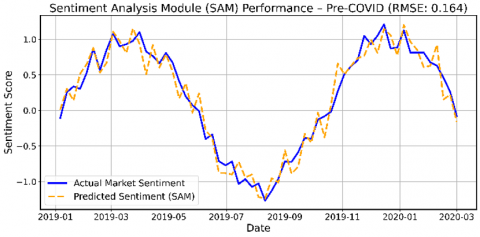
4.6 SAM performance
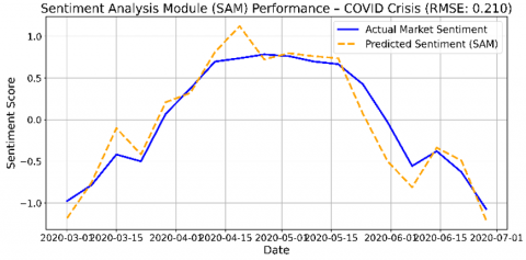
The performance of the SAM is evaluated by comparing its predicted sentiment scores to actual market sentiment trends during both the Pre-COVID and COVID periods. Sentiment scores are normalized to range between -1 and 1, with positive values indicating optimism and negative values reflecting bearish sentiment.
Figure 3 presents a side-by-side time-series comparison of SAM’s predicted sentiment versus actual market sentiment. During the pre-COVID period, SAM exhibits low prediction error and closely tracks sentiment dynamics, demonstrating strong alignment between its textual sentiment outputs and real-world investor behavior.
In contrast, during the COVID period—marked by abrupt sentiment reversals and market volatility—SAM’s prediction error increases. This degradation in accuracy reflects the heightened difficulty of modeling sentiment in crisis environments, where non-linear and sudden shifts are more frequent. The elevated prediction error during the COVID period may stem from increased linguistic noise and misinformation in online discourse during crisis periods.
Nonetheless, SAM continues to deliver valuable directional cues to the overall system.
(a)
(b)
Figure 2. Sector allocation evolution of MPLS during the Pre-COVID period (a) and the COVID period (b)
(a)
(b)
Figure 3. Performance of the SAM during the pre-COVID (stable) period (a) and the COVID (volatile) period (b)
Table 9. Sentiment analysis performance
|
Period |
RMSE |
|
Pre-Covid |
0.164 |
|
COVID |
0.210 |
Prediction accuracy is quantified using Root Mean Squared Error (RMSE) for both periods, with results summarized in Table 9. These metrics confirm SAM’s robustness in normal conditions and its resilience in turbulent markets.
4.7 VFM performance
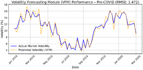
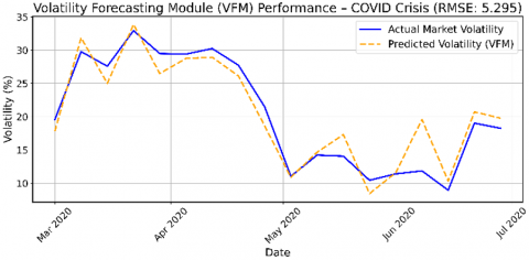
The VFM is assessed by comparing its predicted volatility levels to actual market volatility over the same two periods. Figure 4 illustrates the alignment of VFM predictions with observed volatility data.
(a)
(b)
Figure 4. VFM performance during pre-COVID (a) and COVID crisis (b) periods
In the pre-COVID period, VFM performs with high precision, capturing the temporal structure of volatility with minimal lag. This effectiveness is largely attributed to its hybrid architecture, which combines LSTM-based temporal modeling with Bayesian uncertainty estimation.
During the COVID period, the model faces increased prediction difficulty due to sudden spikes in volatility and deviations from historical norms. Although VFM continues to capture general volatility trends, the prediction error rises, as measured by RMSE values (Table 10).
Table 10. Volatility forecasting performance
|
Period |
RMSE |
|
Pre-Covid |
1.47 |
|
COVID |
5.29 |
These results confirm that VFM is well-suited for risk-aware portfolio construction under stable market conditions and still provides useful, albeit less precise, forecasts during crisis periods.
4.8 GNNs performance
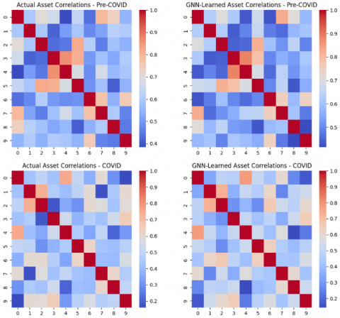
The effectiveness of the GNNs module is evaluated through its ability to learn and represent inter-asset correlations. This is achieved by comparing actual correlation matrices with those learned by the GNN during the Pre-COVID and COVID periods.
Figure 5 displays heatmaps comparing actual and GNN-derived correlation structures, with color gradients indicating the strength and direction of relationships. In the pre-COVID phase, the GNN captures asset interdependencies with high accuracy, enabling enhanced portfolio diversification and informed allocation across sectors.
During the COVID period, market uncertainty introduces greater instability in asset correlations. Despite this, the GNN adapts to the changing structure, learning new patterns that reflect the evolving network of asset relationships.
Quantitative evaluation is conducted using the MAE between the actual and learned correlation matrices. As reported in Table 11, the GNN maintains reasonable accuracy even under turbulent conditions, affirming its utility in modeling systemic relationships in dynamic financial environments.
Figure 5. Comparison of actual vs. GNN-learned asset correlation matrices during pre-COVID and COVID periods
Table 11. GNN learning accuracy
|
Period |
Mean Absolute Error (MAE) |
|
Pre-COVID |
0.041 |
|
COVID |
0.078 |
5.1 Overall performance
The results clearly demonstrate that the MPLS consistently outperforms traditional portfolio optimization models—including Markowitz Mean-Variance Optimization (MVO), single-agent reinforcement learning (RL), and Equal-Weighted Portfolios (EWP)—across both stable and turbulent market environments. This superior performance is most evident in cumulative returns, risk-adjusted metrics (Sharpe and Sortino ratios), and drawdown control.
During the pre-COVID period, MPLS achieved stable portfolio growth by dynamically reallocating assets in response to real-time market signals. It effectively exploited stable asset correlations and low volatility, leveraging its decision modules to maintain high returns while minimizing risk.
In contrast, during the COVID period, MPLS demonstrated robust adaptability to extreme volatility and market uncertainty. The system rapidly adjusted its exposure, reducing risk-heavy positions and reallocating capital toward more resilient sectors. As a result, MPLS maintained competitive returns while limiting drawdowns—a critical advantage over traditional static models during crises.
5.2 Sector allocation adaptability
One of MPLS’s most notable strengths lies in its ability to dynamically reallocate capital across sectors based on macroeconomic shifts and investor sentiment. In stable market conditions, MPLS maintained a diversified sector exposure, adjusting allocations based on historical patterns and underlying economic indicators.
However, during the COVID crisis, the system responded decisively by shifting away from volatile sectors like Technology and increasing its allocation to healthcare. This reallocation mirrors institutional investor behavior and was driven by the integration of sentiment analysis and macro-risk signals. The observed shift demonstrates MPLS’s capacity to detect and act on evolving market regimes, improving resilience and strategic alignment.
These dynamic reallocations underscore MPLS’s effectiveness in synthesizing both quantitative and qualitative signals, allowing it to balance return optimization with risk mitigation in a principled manner.
5.3 Module-level contributions
SAM contributes to MPLS by integrating behavioral finance into the portfolio decision-making process. During the pre-COVID period, it captured investor mood shifts with high accuracy, aligning well with actual sentiment trends. This alignment improved the system’s responsiveness and contributed to enhanced risk-adjusted returns.
In the COVID phase, characterized by erratic sentiment swings, SAM’s predictive accuracy declined, as reflected by higher RMSE values. However, even under such challenging conditions, it provided valuable directional signals that helped guide MPLS’s sector allocation and short-term adjustments, reinforcing the value of sentiment cues in dynamic investment environments.
The VFM is central to MPLS’s risk-aware strategy. In stable markets, it accurately forecasts volatility patterns using a hybrid model that combines temporal learning via LSTMs and uncertainty estimation via Bayesian Networks. This facilitates prudent asset allocation under predictable conditions.
During the COVID crisis, despite facing forecasting challenges due to unprecedented volatility spikes, VFM successfully captured broad volatility trends. Although RMSE values increased, the module continued to play a key role in rebalancing the portfolio away from high-risk assets and enhancing exposure to safer sectors. This demonstrates VFM’s contribution to maintaining system stability even under market stress.
The GNN module significantly enhances MPLS’s ability to model asset-level interdependencies. In the pre-COVID environment, the GNN effectively learned correlation structures that supported improved diversification and sector-wise asset selection.
Although the COVID crisis introduced fragmented and less predictable relationships among assets, the GNN adapted to these changes by recalibrating its learned correlation patterns. The slight increase in MAE during this period reflects the challenge, but GNNs still outperformed static correlation-based approaches. This confirms the value of dynamic graph-based modeling in tracking market structure evolution.
The DFF serves as the integrative engine of MPLS, combining outputs from SAM, VFM, and GNNs into a unified decision vector. Unlike traditional rule-based systems, DFF leverages reinforcement learning (PPO) to dynamically adjust the relative importance of each signal, based on observed market states.
This adaptive weighting mechanism enables the system to shift focus as needed—emphasizing volatility forecasts in high-risk environments, or prioritizing sentiment and structural trends during calmer periods. DFF’s flexibility and contextual awareness are essential to MPLS’s ability to maintain performance while adapting to shifting market regimes, ultimately enhancing both robustness and strategic precision.
While transformer-based RL models offer compelling performance in unstructured environments, MPLS demonstrates competitive results with improved interpretability and lower computational cost. Future work may incorporate temporal attention into agent-level encoders to further enhance signal integration.
5.4 Scalability and real-time deployment
Although MPLS is implemented as an offline daily inference system, latency and scalability remain key considerations for potential real-time deployment. In the current setup, both sentiment extraction and GNN graph updates are executed once per trading day in batch mode, minimizing computational overhead and ensuring temporal consistency.
On standard hardware (NVIDIA T4 GPU with 16 GB RAM), the full inference pipeline—including SAM, VFM, and GNN processing—completes in under 3 minutes. The modular architecture also supports parallel computation across signal modules, which further improves scalability and enables efficient integration into operational pipelines.
Future enhancements will explore streaming-compatible designs and incremental GNN updates to support more responsive, near-real-time decision-making in high-frequency market environments.
This study introduced the MPLS, a hierarchical multi-agent reinforcement learning framework for adaptive portfolio optimization. Empirical results across multiple regimes show that MPLS consistently outperforms traditional methods—including MVO, single-agent RL, and equal-weighted portfolios—achieving notable improvements in returns, drawdown control, and risk-adjusted metrics.
The system’s strength lies in its modular design: SAM captures market sentiment, VFM estimates volatility with uncertainty, and GNNs model structural dependencies. These modules are fused through a PPO-driven DFF, enabling context-aware and explainable allocations.
Despite strong results, MPLS has limitations. It relies on historical data, assumes constant liquidity, and omits execution costs and intraday dynamics. Moreover, its current implementation is limited to equity markets and daily inference.
Future work will focus on modeling transaction frictions, detecting regime shifts, enabling real-time updates, and extending MPLS to broader asset classes. In summary, MPLS offers a robust and scalable foundation for intelligent portfolio decision-making under uncertainty.
[1] Baker, S.R., Bloom, N., Davis, S.J. (2016). Measuring economic policy uncertainty. The Quarterly Journal of Economics, 131(4): 1593-1636. https://doi.org/10.1093/qje/qjw024
[2] Tetlock, P.C. (2007). Giving content to investor sentiment: The role of media in the stock market. The Journal of Finance, 62(3): 1139-1168. https://doi.org/10.1111/j.1540-6261.2007.01232.x
[3] Engle, R. (2002). Dynamic conditional correlation: A simple class of multivariate generalized autoregressive conditional heteroskedasticity models. Journal of Business & Economic Statistics, 20(3): 339-350. https://doi.org/10.1198/073500102288618487
[4] Xu, Y., Guan, B., Lu, W., Heravi, S. (2024). Macroeconomic shocks and volatility spillovers between stock, bond, gold and crude oil markets. Energy Economics, 136: 107750. https://doi.org/10.1016/j.eneco.2024.107750
[5] Markowitz, H. (1952). Portfolio selection. The Journal of Finance, 7(1): 77-91. https://doi.org/10.2307/2975974
[6] Murphy, K.P. (2012). Machine Learning. Cambridge, MA: MIT Press.
[7] Sutton, R.S., Barto, A.G. (2018). Reinforcement Learning: An Introduction, 2nd ed. Cambridge, MA: MIT Press.
[8] Vezhnevets, A.S., Osindero, S., Schaul, T., Heess, N., Jaderberg, M., Silver, D., Kavukcuoglu, K. (2017). FeUdal networks for hierarchical reinforcement learning. arXiv preprint arXiv:1703.01161. https://doi.org/10.48550/arXiv.1703.01161
[9] Schulman, J., Wolski, F., Dhariwal, P., Radford, A., Klimov, O. (2017). Proximal policy optimization algorithms. arXiv preprint arXiv:1707.06347. https://doi.org/10.48550/arXiv.1707.06347
[10] Araci, D. (2019). Finbert: Financial sentiment analysis with pre-trained language models. arXiv preprint arXiv:1908.10063. https://doi.org/10.48550/arXiv.1908.10063
[11] Fischer, T., Krauss, C. (2018). Deep learning with long short-term memory networks for financial market predictions. European journal of Operational Research, 270(2): 654-669. https://doi.org/10.1016/j.ejor.2017.11.054
[12] Feng, F., He, X., Wang, X., Luo, C., Liu, Y., Chua, T.S. (2019). Temporal relational ranking for stock prediction. ACM Transactions on Information Systems (TOIS), 37(2): 1-30. https://doi.org/10.1145/3309547
[13] Huang, G., Zhou, X., Song, Q. (2024). Dynamic optimization of portfolio allocation using deep reinforcement learning. arXiv preprint arXiv:2412.18563. https://doi.org/10.48550/arXiv.2412.18563
[14] Mohammadshafie, A., Mirzaeinia, A., Jumakhan, H., Mirzaeinia, A. (2025). Deep reinforcement learning strategies in finance: insights into asset holding, trading behavior, and purchase diversity. In: Arabnia, H.R., Deligiannidis, L., Amirian, S., Shenavarmasouleh, F., Ghareh Mohammadi, F., de la Fuente, D. (eds) Artificial Intelligence and Applications. CSCE 2024. Communications in Computer and Information Science, vol 2252. Springer, Cham. https://doi.org/10.1007/978-3-031-86623-4_41
[15] Zhang, Y., Zhao, P., Wu, Q., Li, B., Huang, J., Tan, M. (2020). Cost-sensitive portfolio selection via deep reinforcement learning. arXiv preprint arXiv:2003.03051. https://doi.org/10.48550/arXiv.2003.03051
[16] Mnih, V., Kavukcuoglu, K., Silver, D., et al. (2015). Human-level control through deep reinforcement learning. Nature, 518(7540): 529-533. https://doi.org/10.1038/nature14236
[17] Deng, Y., Bao, F., Kong, Y., Ren, Z., Dai, Q. (2016). Deep direct reinforcement learning for financial signal representation and trading. IEEE Transactions on Neural Networks and Learning Systems, 28(3): 653-664. https://doi.org/10.1109/TNNLS.2016.2522401
[18] Almahdi, S., Yang, S.Y. (2017). An adaptive portfolio trading system: A risk-return portfolio optimization using recurrent reinforcement learning with expected maximum drawdown. Expert Systems with Applications, 87: 267-279. https://doi.org/10.1016/j.eswa.2017.06.023
[19] Lillicrap, T.P., Hunt, J.J., Pritzel, A., Heess, N., Erez, T., Tassa, Y., Silver, D., Wierstra, D. (2015). Continuous control with deep reinforcement learning. arXiv preprint arXiv:1509.02971. https://doi.org/10.48550/arXiv.1509.02971
[20] Jiang, Z., Xu, D., Liang, J. (2017). A deep reinforcement learning framework for the financial portfolio management problem. arXiv preprint arXiv:1706.10059. https://doi.org/10.48550/arXiv.1706.10059
[21] Moody, J., Saffell, M. (2001). Learning to trade via direct reinforcement. IEEE Transactions on Neural Networks, 12(4): 875-889. https://doi.org/10.1109/72.935097
[22] Lim, B., Zohren, S. (2021). Time-series forecasting with deep learning: A survey. Philosophical Transactions of the Royal Society A, 379(2194): 20200209. https://doi.org/10.1098/rsta.2020.0209
[23] Wu, H., Xu, J., Wang, J., Long, M. (2021). Autoformer: decomposition transformers with auto-correlation for long-term series forecasting. arXiv preprint arXiv:2106.13008. https://doi.org/10.48550/arXiv.2106.13008
[24] Bacon, P.L., Harb, J., Precup, D. (2017). The option-critic architecture. Proceedings of the AAAI Conference on Artificial Intelligence, 31(1): 1726-1734. https://doi.org/10.1609/aaai.v31i1.10916
[25] Uddin, A., Tao, X., Yu, D. (2023). Attention based dynamic graph neural network for asset pricing. Global Finance Journal, 58: 100900. https://doi.org/10.1016/j.gfj.2023.100900
[26] Nassirtoussi, A.K., Aghabozorgi, S., Wah, T.Y., Ngo, D. C.L. (2014). Text mining for market prediction: A systematic review. Expert Systems with Applications, 41(16): 7653-7670. https://doi.org/10.1016/j.eswa.2014.06.009
[27] Finance, Y. (2022). Yahoo finance-stock market live, quotes, business & finance news. Dipetik 5/7/2021, dari.
[28] Bloomberg Middle East. https://www.bloomberg.com/middleeast, accessed on Feb. 5, 2025.
[29] Investing.com - Stock Market Quotes & Financial News. https://www.investing.com/, accessed on Feb. 5, 2025.