Mustafa T. Hussein*![]() | Ameen M. Al-Juboori
| Ameen M. Al-Juboori![]() | Sarah Z. Mahdi
| Sarah Z. Mahdi![]() | Essam Z. Fadhil
| Essam Z. Fadhil![]() | Salah Amroune
| Salah Amroune![]() | Amina Zohra Akkal
| Amina Zohra Akkal![]()
© 2025 The authors. This article is published by IIETA and is licensed under the CC BY 4.0 license (http://creativecommons.org/licenses/by/4.0/).
OPEN ACCESS
In this article, the modeling and model-based control of a motorcycle like inverted pendulum system with a gyroscope controller are addressed. The mathematical model of the system which includes an inverted pendulum and two gyroscopic flywheels is derived using the Lagrange equations. A problem arising from the derived dynamic model is that the system is highly nonlinear and unstable. Hence, the derived model is linearized to obtain a state-space model. Based on the linearized model, a controller and a state observer are designed. The controller is designed to generate required moment for stabilization using the two flywheel gyroscopes in the system. The observability and controllability of the designed observer and controller is verified based on the locations of the system eigenvalues. Several simulations are carried out in this work using the derived state-space model and the designed controller to ensure the efficiency of the model-based controlled system.
inverted pendulum system, motorcycle-like robot, gyroscopic control, Lagrangian modeling, nonlinear dynamics, system linearization
Urban environments are increasingly burdened by traffic congestion, limited parking, and air pollution, which have prompted growing interest in compact, smart, and environmentally friendly transportation alternatives [1]. Among these, motorcycles are widely used due to their lightweight and narrow profile, offering improved maneuverability and fuel efficiency. However, motorcycles are also among the most accident-prone vehicles due to their poor inherent stability, particularly when stationary or at low speeds. In response to global road safety concerns, the United Nations launched the Decade of Action for Road Safety 2021-2030, aiming to reduce fatalities through innovative safety solutions [2].
From a control systems perspective, a motorcycle behaves similarly to an inverted pendulum an unstable and nonlinear system that has served as a benchmark problem for testing advanced control algorithms [3]. Numerous configurations of inverted pendulum systems have been studied, including single-link, double, and triple pendulum models, as well as systems incorporating inertial wheels and gyroscopes [4-8]. Yet, many of these systems rely on external force or torque input from stationary platforms or mobile carts, rendering them unsuitable for self-balancing motorcycle applications. A well-known commercial application of inverted pendulum control is the Segway two-wheeled vehicle.
Counterbalancing mechanisms such as inertial wheels and Control Moment Gyroscopes (CMGs) have been proposed for improving balance in single-track vehicles [9-11]. Recent reviews have explored the application of CMGs as stabilization mechanisms in electric two-wheelers, highlighting their potential integration into Intelligent Balance Assistance Systems (IBAS). Pedapati and Chidambaram [12] provided a comprehensive overview of gyroscopic configurations, advanced control strategies, and sensor fusion approaches for enhancing the stability and adaptability of two-wheeled vehicles in real-world traffic conditions. While CMGs offer effective dynamic stabilization, challenges such as energy consumption and mechanical complexity remain key barriers to widespread implementation. Their work also emphasized the importance of networking and vehicle-to-infrastructure communication in developing smart, self-balancing electric two-wheelers. Inertial wheels operate by adjusting rotational acceleration, but they require high-performance motors and often struggle with real-time disturbances. Aranovskiy et al. [13] focused on the dynamic stabilization of a two-dimensional inverted pendulum using a scissored pair of CMGs. This configuration was motivated by applications in non-anthropomorphic bipedal robots, where such simplified pendulum dynamics can approximate the robot's motion. The researchers developed a mathematical model of the inverted pendulum that intentionally omits non-essential dynamics to allow for analytical tractability and control design. A linear control law was designed based on this simplified model, and the team conducted experimental validation to demonstrate its effectiveness in maintaining upright balance. The work emphasizes the feasibility of using scissored CMG systems for lightweight, real-time balance control in robotics, particularly in situations where traditional actuation methods are not practical. In contrast, CMGs use the principle of angular momentum conservation to resist changes in orientation, offering better stability and disturbance rejection [3]. These systems have been successfully applied in spacecraft attitude control and ship stabilization and are now being explored in terrestrial mobility platforms. Badgujar and Mohite [14] designed, implemented, and tested a CMG mechanism for self-balancing an electric moped (Okinawa IPRAISE Scooter), capable of maintaining stability both when stationary and in motion. The system uses two continuously spinning flywheels driven by DC motors around the vertical axis, paired with stepper motor-driven gimbals to generate corrective torque about the horizontal axis. A feedback loop with an IMU sensor and a PID controller provides dynamic balance correction by sensing tilt and adjusting gimbal motion.
The CMG mechanism demonstrated superior performance compared to traditional stabilization approaches like steering control or mass shifting, due to its torque amplification and momentum storage capacity. Simulation and analysis were performed using CREO for modeling and ANSYS for structural evaluation. Despite increased power consumption (+10%), added weight (+25%), and cost (+9%), the mechanism proved to be a compact and effective solution for enhancing ride stability, particularly in urban or uneven road conditions. Zheng et al. [15] presented a dynamic modeling and control approach for an unmanned motorcycle that integrates both steering actuation and a dual CMG system to improve stability. Unlike earlier studies that lock the steering mechanism and rely solely on CMG-based inverted pendulum models, this work emphasizes the importance of utilizing steering as an additional stabilizing component.
The authors developed a multibody dynamic model using Lagrange equations of the first kind for accurate physical simulation. For control design, a simplified model was derived, enabling the development of a combined balance controller that coordinates inputs from both the steering system and dual CMGs. Simulation results confirmed that the combined control strategy significantly outperformed both standalone steering and traditional CMG-only control systems in terms of roll stabilization and maneuverability. Jin et al. [3] proposed a novel inverted pendulum system that utilizes the gyroscopic precession effect as its core stabilization mechanism. Unlike traditional inertia-wheel pendulum systems which rely on accelerating and decelerating a flywheel to generate torque their design offers a more efficient, responsive, and compact alternative. The system leverages a high-speed gyroscopic rotor to produce significant precession torque, enabling rapid and stable equilibrium control. Both disturbance-free and disturbance-response experiments were conducted using a physical prototype, demonstrating effective stabilization and strong anti-interference performance. Additionally, the stabilizing mechanism was successfully applied to a bicycle posture control system, validating its practical applicability and robustness.
Recent advancements, such as Honda’s Riding Assist technology, demonstrate the feasibility of motorcycle self-balancing using gyroscopic systems. However, most existing works focus on single-gyroscope configurations, leaving a clear gap in the literature concerning the modeling and control of dual-gyroscope systems for enhanced stabilization.
To address this gap, this paper presents the modeling and control of a motorcycle-like inverted pendulum system using two counter-rotating flywheel gyroscopes. The dynamic model is formulated via the Euler-Lagrange approach and subsequently linearized to facilitate controller design. A Linear Quadratic Regulator (LQR) controller, in combination with a Kalman filter, is developed to stabilize the roll motion of the system. It is important to clarify that the presented system is a scaled-down prototype, with parameters such as the 1.25 kg body mass selected for simulation and controller validation purposes. The key contributions of this study include: the development of a dual-gyroscope dynamic model, observer-based LQR control system design, and validation of stabilization performance through simulations under various disturbance conditions.
This section aims to explain the stages of the system modeling carried out, namely mathematical modeling, three-dimensional modeling, determining the parameters used, and the stages of system design.
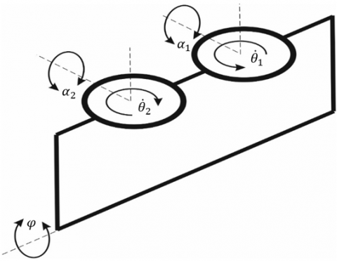
The general model of inverted pendulum as shown in Figure 1 has a mechanical base of inverted pendulum which consists of the following parts:
(i) Base of the inverted pendulum.
(ii) Mechanical rotating flywheel gyroscopes.
Figure 1. The sketch of the inverted pendulum system with double gyroscopes
Given the dynamics and size of the inverted pendulum, the balancing torque required to stabilize the pendulum is estimated.
The system can be made in two ways, namely by using one or two flywheel gyroscopes. Considerations in this research prefer to use two flywheel gyroscopes rather than one because to get mass properties so as to increase the value of precession torque, the greater the effect of the gyroscope produced will provide torque roll-motion inverted pendulum to maintain stability when deviating from its upright position.
2.2 Rigid body dynamics
In this research the use the Euler-Lagrange approach is implemented [8], which considers the system as a whole. Two key terms in this process are generalized variables and generalized forces. The main idea of this procedure is to find expressions for the total kinetic energy (T) and total potential energy (V) of the system. potential energy (V) of the system. Then, the equations of motion will be determined by solving the generalized equations of motion. The Lagrange formula is [16]:
$\frac{d}{d t}\left(\frac{\partial L}{\partial q_i}\right)-\frac{\partial L}{\partial q_i}=Q_i$
where, $q_i$ are generalized coordinates, $Q_i$ are generalized forces, and $L=T-V$ is the Lagrangian. In this study, the generalized coordinates are the roll angle $q_1=\varphi$ of the inverted pendulum and the precession angle of the gyroscope is $q_2=\alpha$. Therefore, a 2nd order differential equation can be obtained which is written with equation [17]:
$\left[\frac{d}{d t}\left(\frac{\partial T}{\partial \dot{q}_{\imath}}\right)-\frac{\partial T}{\partial q_1}\right]-\left[\frac{d}{d t}\left(\frac{\partial V}{\partial \dot{q}_1}\right)-\frac{\partial V}{\partial q_1}\right]=Q_1$
$\left[\frac{d}{d t}\left(\frac{\partial T}{\partial \dot{q}_2}\right)-\frac{\partial T}{\partial q_2}\right]-\left[\frac{d}{d t}\left(\frac{\partial V}{\partial \dot{q}_2}\right)-\frac{\partial V}{\partial q_2}\right]=Q_2$
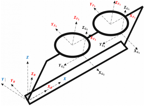
Figure 2. Sketch diagram of the system coordinates
Figure 2 illustrates an coordinates view of the system. It is assumed that the inverted pendulum consists of a main body (B), gyro-cages (G) and gyro-flywheel (F), then the total kinetic energy and total potential energy can be expressed as [18-22]:
$\begin{aligned} & T=T_B+T_{G 1}+T_{F 1}+T_{G 2}+T_{F 2} \\ & V=V_B+V_{G 1}+V_{F 1}+V_{G 2}+V_{F 2}\end{aligned}$
Before determining each part of the kinetic energy, first create a list table for the static inverted pendulum parameters (Table 1).
Furthermore, the velocity variables that occur are as follows:
$\omega_{G_i}=\left(\dot{\varphi} \cos \alpha_i\right) x_{G_i}+\dot{\alpha_{\imath}} y_{G_i}+\left(\dot{\varphi} \sin \alpha_i\right) z_{G_i}$
$\omega_{F_i}=\left(\dot{\varphi} \cos \alpha_i\right) x_{F_i}+\dot{\alpha}_l y_{F_i}+\left(\dot{\varphi} \sin \alpha_i\right) z_{F_i}+\dot{\theta} z_{F_i}$
The kinetic energy at each part of the inverted pendulum can be expressed by equation as follows:
$T_B=\frac{1}{2} m_B\left(\dot{\varphi} h_B\right)^2+\frac{1}{2} I_{B x x} \dot{\varphi}^2$
$T_{G_i}=\frac{1}{2} m_{G_i}\left(\dot{\varphi} h_{G_i}\right)^2+\frac{1}{2}\left[I_{G_i x}\left(\dot{\varphi} \cos \alpha_i\right)^2+I_{G_i y}\left(\dot{\alpha}_i\right)^2+I_{G_i z}\left(\dot{\varphi} \sin \alpha_i\right)^2\right]$
$T_{F_i}=\frac{1}{2} m_{F_i}\left(\dot{\varphi} h_{F_i}\right)^2+\frac{1}{2}\left[I_{F_i x}\left(\dot{\varphi} \cos \alpha_i\right)^2+I_{F_i y}\left(\dot{\alpha}_i\right)^2+I_{F_i z}\left(\dot{\varphi} \sin \alpha_i+\dot{\theta}_i\right)^2\right]$
Table 1. Static inverted pendulum parameters
|
Parameter |
Symbol |
|
Body mass and height of center of gravity (COG) |
$m_B, l_B$ |
|
Gyro- mass and height of COG |
$m_G, l_G$ |
|
Gyro- flywheel and mass of COG |
$m_F, l_F$ |
|
Body inertia |
$I_{B x}$ |
|
Gyro-cover inertia |
$\left[\begin{array}{lll}I_{G x} & I_{G y} & I_{G z}\end{array}\right]$ |
|
Gyro-flywheel inertia |
$\left[\begin{array}{lll}I_{F x} & I_{F y} & I_{F z}\end{array}\right]$ |
|
Gravity acceleration |
$g$ |
|
Flywheel rotation speed |
$\dot{\theta}$ |
Total kinetic energy can be found with the following equation
$T=\left[T_B\right]+\left[T_{G 1}+T_{F 1}\right]+\left[T_{G 2}+T_{F 2}\right]$
$\begin{aligned} T=\frac{1}{2} m_B\left(\varphi h_B\right)^2+\frac{1}{2}\left[I_{B x}(\varphi)^2\right] & +\frac{1}{2} m_{G_1}\left(\dot{\varphi} h_{G_1}\right)^2+\frac{1}{2}\left[I_{G_1 x}\left(\dot{\varphi} \cos \alpha_1\right)^2+I_{G_1 y}\left(\dot{\alpha}_1\right)^2+I_{G_1 z}\left(\dot{\varphi} \sin \alpha_1\right)^2\right] \\ & +\frac{1}{2} m_{F_1}\left(\dot{\varphi} h_{F_1}\right)^2+\frac{1}{2}\left[I_{F_1 x}\left(\dot{\varphi} \cos \alpha_1\right)^2+I_{F_1 y}\left(\dot{\alpha}_1\right)^2+I_{F_1 z}\left(\dot{\varphi} \sin \alpha_1+\dot{\theta}_1\right)^2\right] \\ & +\frac{1}{2} m_{G_2}\left(\dot{\varphi} h_{G_2}\right)^2+\frac{1}{2}\left[I_{G_2 x}\left(\dot{\varphi} \cos \alpha_2\right)^2+I_{G_2 y}\left(\dot{\alpha}_2\right)^2+I_{G_2 z}\left(\dot{\varphi} \sin \alpha_2\right)^2\right] \\ & +\frac{1}{2} m_{F_2}\left(\dot{\varphi} h_{F 2}\right)^2+\frac{1}{2}\left[I_{F_2 x}\left(\dot{\varphi} \cos \alpha_2\right)^2+I_{F_2 y}\left(\dot{\alpha}_2\right)^2+I_{F_2 z}\left(\dot{\varphi} \sin \alpha_2+\dot{\theta}_2\right)^2\right]\end{aligned}$
The potential energy at each part of the inverted pendulum can be expressed by equation as follows:
$\begin{aligned} V_B & =m_B . g . h_B \cos \varphi \\ V_{G i} & =m_{G_i} . g . h_{G_i} \cos \varphi \\ V_{F i} & =m_{F i} . g . h_{F i} \cos \varphi\end{aligned}$
Total potential energy can be known by the following equation:
$V=\sum_{i=1}^N m_i . g . h_i=\left[h_B m_B+2 h_G m_G+2 h_F m_F\right] g \cos (\varphi)$
Application of the kinetic energy and potential energy system equations to the Lagrangian equations of motion described earlier, so that we obtain the combination of two non-linear differential equations:
$\begin{aligned} \ddot{\varphi}\left[h_B^2 m_B+2 h_G^2 m_G+2 h_F^2\right. & \left.m_F+I_{B x}+2 \cos ^2(\varphi)\left(I_{G x}+I_{F x}\right)+2 \sin ^2(\alpha)\left(I_{G z}+I_{F z}\right)\right] \\ & -4 \dot{\varphi} \dot{\alpha} \cos (\alpha) \sin (\alpha)\left[I_{G x}+I_{F x}-I_{G z}-I_{F z}\right]+2 \dot{\theta} \cos (\alpha) \dot{\alpha} I_{F z} \\ & -\left[h_B m_B+2\left(h_G m_G\right)+2\left(h_F m_F\right)\right] g \sin (\varphi)=Q_1\end{aligned}$
$2 \ddot{\alpha}\left(I_{G y}+I_{F y}\right)+2 \dot{\varphi}^2 \cos (\alpha) \sin (\alpha)\left[I_{G x}-I_{G z}+I_{F x}-I_{F z}\right]-2 \dot{\varphi} \cos (\alpha) \dot{\theta} I_{F z}=Q_2$
where by defining the above equation:
$\begin{gathered}c=\cos \\ s=\sin \\ a_1=2\left(I_{G x}+I_{F x}\right) \\ a_2=2\left(I_{G y}+I_{F y}\right) \\ a_3=2\left(I_{G z}+I_{F z}\right) \\ a_4=I_{B x} \\ a_5=k_1-k_3 \\ a_6=h_B m_B+2\left(h_G m_G\right)+2\left(h_F m_F\right) \\ a_7=h_B^2 m_B+2 h_G^2 m_G+2 h_F^2 m_F\end{gathered}$
The application of the equation of motion can be written as follows:
$\ddot{\varphi}\left[a_4+a_7+a_1 c^2 \alpha+a_3 s^2 \alpha\right]-2 a_5 \dot{\varphi} \dot{\alpha} c \alpha s \alpha+2 \dot{\theta} c \alpha \dot{\alpha} I_{F z}-a_6 g s \varphi=Q_1$
$a_2 \ddot{\alpha}+a_5 \dot{\varphi}^2 c \alpha s \alpha-2 \dot{\varphi} c \alpha \dot{\theta} I_{F z}=Q_2$
where, $Q_i$ is the generalized forces.
$\begin{gathered}Q_1=h_B F_d \cos \varphi \\ Q_2=M_u\end{gathered}$
where, $Q_i$ is the general non-conservative force. $F_d$ represents the horizontal disturbance applied to the inverted pendulum as well as the model dynamics uncertainty, and $M_u$ denotes the torque generated by the DC motor.
2.3 Linearized full system dynamics
The study investigates the inverted pendulum system and validates the performance of controllers designed to stabilize a single-track vehicle by using the gyroscopic effects generated by two counter-rotating flywheels. The system is linearized around the upright equilibrium point, defined by a roll angle φ = 0 and a gimbal angle α = 0, while the flywheels rotate in opposite directions at a constant speed of 500 rpm. Accordingly, the linearization of the dynamic model is performed based on these equilibrium conditions:
$x=\left[\begin{array}{llllll}\varphi & \dot{\varphi} & \alpha_1 & \dot{\alpha}_1 & \alpha_2 & \dot{\alpha}_2\end{array}\right]$
Assuming the system with no input ($M_u=0$) and no disturbance ($F_d=0$), then the equilibrium points in the system in the upright position produce the numerical result for the linear model is:
$\dot{x}=\left[\begin{array}{cccccc}0 & 1 & 0 & 0 & 0 & 0 \\ \frac{g . k_6}{k_1+k_7+k_4} & 0 & 0 & -\frac{I_{F_1 z} \dot{\theta}_1}{k_1+k_7+k_4} & 0 & -\frac{I_{F_2 z} \dot{\theta}_2}{k_1+k_7+k_4} \\ 0 & 0 & 0 & 1 & 0 & 0 \\ 0 & \frac{I_{F_1 z} \dot{\theta}_1}{I_{F_1 y}+I_{G_1 y}} & 0 & 0 & 0 & 0 \\ 0 & 0 & 0 & 0 & 0 & 1 \\ 0 & \frac{I_{F_2 z} \dot{\theta}_2}{I_{F_2 y}+I_{G_2 y}} & 0 & 0 & 0 & 0\end{array}\right] x+\left[\begin{array}{ccc}0 & 0 \\ 0 & 0 \\ 0 & 0 \\ \frac{1}{I_{F_1 y}+I_{G_1 y}} & 0 \\ 0 & 0 \\ 0 & \frac{1}{I_{F_2 y}+I_{G_2 y}}\end{array}\right] u$
where, $x_1$ represents the roll angle of inverted pendulum, $x_2$ is angular velocity of roll inverted pendulum, $x_3$ denotes the inclination angle of gyroscope 1, $x_4$ is the angular velocity of precision gyroscope 1, $x_5$ is the precision angle of gyroscope 2, $x_6$ is the correspond to the angular velocity of precision gyroscope 2. The control input u is the input torque generated by the flywheel gyroscopes. The constants used in the linearized dynamic equations are defined to simplify the representation of mass, inertia, and gyroscopic effects. Specifically, k1=mb.lb2 represents the moment of inertia of the main body about the pivot axis; k2=mb.g.lb accounts for the gravitational torque acting on the pendulum body; and k3=If.ωf denotes the gyroscopic torque produced by the rotating flywheel, where If is the flywheel inertia and ωf is its angular speed. Additionally, k4=mg.lg2 represents the inertia of the gyroscope housing, k5=Ig.ωf corresponds to the gyroscopic precession torque generated by the gimbal system, and k6 is a composite term that aggregates the total moment of inertia from the gimbal and flywheel assemblies, including coupling effects. These constants are integrated into the linear state-space model to express the system matrices A and B compactly for control design. These constants represent grouped terms involving mass (m), lengths (l), and inertias (I), introduced for notational simplicity in the linearized matrix expressions.
Inverted pendulum is a system that under normal circumstances has an unstable condition and will tend to fall. In order to stabilized, an additional device or force is needed to counteract the force that causes the inverted pendulum to fall. Gyroscopic uses principle of the gyroscope effect produced by a rotating disk as shown in Figure 1.
As seen in Figure 1, a disk with mass that has inertia equal to I rotates about the z-axis with angular velocity ($\dot{\theta}$). If on y-axis there is an angular change of $\dot{\alpha}$ as shown in Figure 2 then the torque generated on the axis can be found by using equation of state space.
Based on the state space model derived earlier control system will be designed in order to determine how much precession torque is given to the inverted pendulum to meet the desired equilibrium point [17].
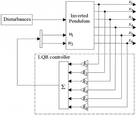
3.1 LQR control system design
The control used to control the stability in roll angle in this research is LQR. LQR controller design can be seen in Figure 3. LQR control system will be designed for the system, so that it can be applied to control the roll angle around the equilibrium point. In the calculation of the mathematical model, the state space equation is obtained as in equation below, in the LQR control design using the equation that has been diluted.
Figure 3. Block diagram of LQR controller
LQR control design uses equations that have been linearized by assuming the inverted pendulum deviation angle does not exceed the maximum degree boundaries or is considered to have very small changes. So that after the parameters are entered in the state space model, the state space with linear plant numerical form will be used to find the eigenvalues of the system to ensure stability [22-24].
The value of gain K which represent the controller gain matrix; is said to be optimal if it is able to combine the efficiency of energy use and performance. This energy efficiency will be shown by how much control torque/precision torque is needed in the simulation to maintain the stability of the inverted pendulum. Meanwhile, performance is said to be good if it is still able to prevent the inverted pendulum from falling.
The controller gain is designed using linear quadratic regulator in a way to minimize the following cost equation:
$J=\int_0^{\infty} e^2 d t=\frac{1}{2} \int_0^{\infty}\left[x^T Q_c x+u^T R_c u\right] d t$
The ideal values of the controller's $Q_c$ and $R_c$ matrices are obtained by trial and error since there is no unique solution for these matrices. The selection of these matrices depends on how much influence y and u are desired on the cost function. What needs to be considered in this trial-and-error process is that matrix $Q_c$ and $R_c$ must be symmetric and positive definite. The controller gain is calculated using the Riccati Equation:
$K=R^{-1} B^T P=\left[\begin{array}{llllll}k_1 & k_2 & k_3 & k_4 & k_5 & k_6\end{array}\right]$
$k_i$ is $[2 \times 1]$ matrix, P is determined using the system matrices and the $Q_c$, $R_c$ matrices as follows:
$A^T P+P A+Q_c-P B R_c^{-1} B^T P=0$
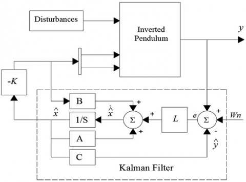
Furthermore; a Kalman filter is designed to estimate the unmeasured states of the system [8]. The value of Kalman gain L and LQR gain K will be calculated to obtain a good Control response. The diagram of the mathematical model with Control LQR is shown in Figure 4. The $Q_c$ matrix in the LQR controller will also be designed to prioritize the roll state as the most significantly affected state.
Figure 4. Block diagram of the system with observer and controller
The system parameters used in the simulation is addressed in the Table 2. These parameters are submitted in state space equation stated earlier which represent the full state space model of the system. The induced constant system matrices used to check the controllability and observability of the system and also to design the controller and observer gains for simulations.
By using the MATLAB program, the controllability matrix is obtained with determinant value is not equal to zero Because the controllability matrix has a full rank of 6, so it can be used to prove the controllability of the system rank of 6, thus it can be concluded that the system can be controlled. The observability matrix is also calculated using the MATLAB program the observability matrix is obtained with the value of the determinant not equal to zero. determinant is not equal to zero because the observability matrix has a full rank of 6, which is 6, thus it can be concluded that the system is observable.
Table 2. The system parameters and units
|
No. |
Parameter |
Symbol |
Value |
Units |
|
1 |
Body mass |
$m_B$ |
1.25 |
kg |
|
2 |
COG Body |
$h_B$ |
0.08 |
m |
|
3 |
Inertia $B_{x x}$ |
$I_{B x}$ |
0.005 |
kg, m2 |
|
4 |
Flywheel Mass 1 & 2 |
$m_F$ |
0.25 |
kg |
|
5 |
COG Flywheel |
$h_F$ |
0.08 |
m |
|
6 |
Inertia $F_{x x}$, $F_{y y}$, $F_{z z}$ |
$I_{F x}, I_{F y}, I_{F z}$ |
(0.00034; 0.00034; 0.00067) |
kg, m2 |
|
7 |
Gyroscope Mass 1 & 2 |
$m_G$ |
0.3 |
kg |
|
8 |
COG Gyroscope |
$h_G$ |
0.09 |
m |
|
9 |
Inertia $G_{x x}$, $G_{y y}, G_{z z}$ |
$I_{G x}, I_{G y}, I_{G z}$ |
(0.00057; 0.00036; 0.0009) |
kg, m2 |
|
10 |
Rotational Speed Flywheel 1 |
$\dot{\theta}_1$ |
3000 |
rpm |
|
11 |
Rotational Speed Flywheel 2 |
$\dot{\theta}_2$ |
-3000 |
rpm |
|
12 |
Gravitational coefficient |
g |
9.81 |
m/s2 |
The weight matrices are $Q_c$ and $R_c$ matrices. The selection of $Q_c$ and $R_c$ matrices is done by trial and error. With the condition that the $Q_c$ matrix is symmetrical, positive semidefinite and real ($Q_c$ > 0). Matrix $Q_c$ is a matrix [6 × 6] and diagonal matrix, and when separation will be obtained identity matrix multiplied by a constant. While the matrix R is a symmetrical matrix, positive definite and real ($R_c$ > 0). Matrix $R_c$ is a matrix of order [2 × 2] and a diagonal matrix, and when the separation will be obtained identity matrix multiplied by constant. To get the gain K, first determine the weights that will be used for each output of the system/plant. Weights are used to prioritize which outputs should have more priority to be improved. The values of $Q_c$ and $R_c$ matrices are selected as follow:
$Q_c=\left[\begin{array}{cccccc}100 & 0 & 0 & 0 & 0 & 0 \\ 0 & 10 & 0 & 0 & 0 & 0 \\ 0 & 0 & 100 & 0 & 0 & 0 \\ 0 & 0 & 0 & 1 & 0 & 0 \\ 0 & 0 & 0 & 0 & 100 & 0 \\ 0 & 0 & 0 & 0 & 0 & 1\end{array}\right]$
$R_c=\left[\begin{array}{ll}1 & 0 \\ 0 & 1\end{array}\right]$
From Riccati Equation, the matrix P will be known. Matrix P is the solution matrix of the Ricccati equation. If the values of matrix P are known, then substituted into costfunction equation, so that the value of the optimal feedback matrix (K) that minimizes the cost function J can be found.
The amount of data available in the calculation of the optimal control vector value K requires the help of a computer program, in this case MATLAB is used.
Calculations using MATLAB can be known feedback value K optimal system based on the system model. The calculation obtained the value of the optimal feedback gain matrix for the system value:
$K=\left[\begin{array}{cccccc}-18.13 & -2.89 & 0 & 1 & 10 & 0 \\ 18.13 & 2.89 & 10 & 0 & 0 & 1\end{array}\right]$
By the same procedure the Kalman filter matrix is also determined as:
$L=\left[\begin{array}{cccccc}0 & 0 & 0 & 0 & 0 & 0 \\ 0 & 0 & 0 & 0 & 0 & 0 \\ 0 & 0 & 0 & 0 & 0 & 0 \\ 0 & 0 & 0 & 0 & 0 & 0 \\ 0 & 0 & 0 & 3.6 & 0 & 0 \\ 0 & 0 & 0 & 0 & 0 & 3.6\end{array}\right]$
Using the mathematical model derived and the controller and observer designed based on the derived model the simulation of the system is done. The system is tested first using the eigenvalues by comparing the derived eigenvalues model and the controlled system eigenvalues as shown in the Table 3. It is clear from the values in the table that the derived model is unstable, while the controlled model is asymptotic stable system.
Table 3. The system eigenvalues comparison
|
System Eigenvalues |
Controlled System Eigenvalues |
|
0 |
-81999929.65 |
|
0 |
-81999989.99 |
|
0 |
-63.96 |
|
0.0 + 117.38i |
-3.19 + 1.66i |
|
0.0 - 117.38i |
-3.19 - 1.66i |
|
0 |
-10.00 |
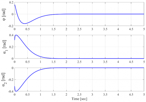
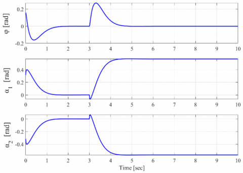
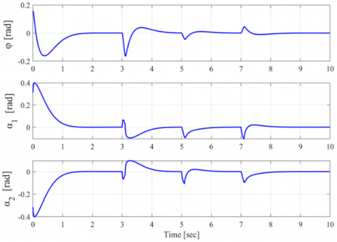
The system then simulated after the prove of the controllability check, several simulation results is presented based on the designed controller and observer. First simulation is shown in Figure 5. In this simulation results, the system given initial conditions as $x=\left[\begin{array}{llllll}\frac{p i}{20} & 0 & \frac{p i}{10} & 0 & -\frac{p i}{10} & 0\end{array}\right]$, makes the controller recover stability and eliminates the inclement of the motorcycle. The observer designed successfully estimates the states of the system and overcomes the error due to the unknown initial conditions in the states. After that the initial conditions is set as the same as in the first simulation $x=\left[\begin{array}{llllll}\frac{p i}{20} & 0 & \frac{p i}{10} & 0 & -\frac{p i}{10} & 0\end{array}\right]$, and the system also is subjected to step disturbance in all rotation variables $\varphi=9, \alpha_1=18, \alpha_2=-18$ degrees respectively as shown in Figure 6. This disturbance is used complicate the simulation situation on the observer and the controller. It can be noted from the Figure 6 which shows the second case of the simulation that the controller based on the observed states eradicate the effect of the disturbance effect very fast. In the third set of simulation (Figure 7) the model is tested under impulse disturbance on the $\varphi$, $\alpha_1$, and $\alpha_2$. The disturbances divided along time. The roll angle of inverted pendulum is subjected to Impulse disturbance at time 3 sec from the simulation, the inclination angle of the gyroscope 1 and 2 is subjected to impulse disturbance at 5th and the 7th sec of the simulation time. The disturbance is assumed as disturbance angle effect for instance (0.1 sec) on the each of the system variables the disappears. The behavior of the controller in this case is perfectly evade the effect of the impulse disturbance and keep the system stable although several impulse disturbances. From the all simulations figures it can be concluded that the controller keeps the roll angle of the pendulum always equal to zero which is the main setpoint of the motorcycle.
The results presented in this study clearly indicate that the model has only been simulated. In the case of experimental implementation, several practical challenges may arise. Specifically, the system parameters are likely to change, necessitating a redesign of the controllers and observer gain matrices. Additionally, issues such as measurement noise, mechanical constraints, and torque requirements must be taken into account during the design of both the controller and the observer.
Figure 5. Controlled system test against the change in initial conditions
Figure 6. Controlled system test against the step disturbance
Figure 7. Controlled system test against impulse disturbance
A physical model for a gyroscopic inverted pendulum system equipped with two gyroscopes was developed. Theoretical analysis and simulation results showed that increasing the flywheel rotation speed leads to a faster response in achieving equilibrium. The dual-gyroscope system demonstrated a more effective and rapid stabilization response compared to single-gyroscope configurations. The simulation results further confirmed that the LQR controller successfully maintained the roll angle of the inverted pendulum near zero degrees under various disturbances. This zero-degree setpoint represents the upright posture, which is particularly relevant during low-speed operation or when the vehicle is stationary conditions in which motorcycles are most vulnerable to tipping.
However, the scalability of the proposed system to full-size motorcycles introduces key engineering challenges. Real motorcycles have significantly higher mass and inertia, requiring larger gyroscopic devices capable of generating sufficient precession torque. This raises concerns about the gyroscope's physical size, energy consumption, and compatibility with the motorcycle's frame and existing vehicle dynamics. Furthermore, the continuous energy demand for high-speed rotation may impact power efficiency, particularly in electric two-wheelers.
The current controller design and simulations represent an important step, but experimental validation on a scaled prototype is essential to assess practical feasibility. Future work should also investigate the robustness of the control system under sensor noise, dynamic modeling uncertainties, and sudden external disturbances. Moreover, it is recommended to explore hybrid or adaptive control architectures that combine CMG stabilization with rider inputs and steering control for full-speed operation.
Finally, a comparative analysis with other stabilization approaches such as single CMG systems, reaction wheels, and active steering methods should be conducted to quantify the advantages and trade-offs of the dual-CMG design. These future developments will play a crucial role in realizing intelligent, self-balancing two-wheeled vehicles for real-world applications.
[1] Olivares, M., Albertos, P. (2014). Linear control of the flywheel inverted pendulum. ISA Transactions, 53(5): 1396-1403. https://doi.org/10.1016/j.isatra.2013.12.030
[2] World Health Organization. (2021). Decade of action for road safety 2021–2030. https://www.who.int/teams/social-determinants-of-health/safety-and-mobility/decade-of-action-for-road-safety-2021-2030.
[3] Jin, H., Yang, D., Liu, Z., Zang, X., Li, G., Zhu, Y. (2015). A gyroscope-based inverted pendulum with application to posture stabilization of bicycle vehicle. In 2015 IEEE International Conference on Robotics and Biomimetics (ROBIO), Zhuhai, China, pp. 2103-2108. https://doi.org/10.1109/ROBIO.2015.7419084
[4] Dhulkefl, E.J., Mahmood, Z.S., Nasret, A.N., Mohammed, A.B. (2023). A new method investigation for robotic inverted pendulum movement and control. Journal Européen des Systèmes Automatisés, 56(6): 1065-1071. https://doi.org/10.18280/jesa.560616
[5] Mourad, A., Zennir, Y., Tolba, C. (2022). Intelligent and robust controller tuned with WOA: Applied for the inverted pendulum. Journal Européen des Systèmes Automatisés, 55(3): 359-366. https://doi.org/10.18280/jesa.550308
[6] Lee, T., Ju, D., Lee, Y.S. (2025). Transition control of a double-inverted pendulum system using Sim2Real reinforcement learning. Machines, 13(3): 186. https://doi.org/10.3390/machines13030186
[7] Rani, M., Kamlu, S.S. (2025). Optimal LQG controller design for inverted pendulum systems using a comprehensive approach. Scientific Reports, 15: 4692. https://doi.org/10.1038/s41598-025-85581-3
[8] Al Juboori, A.M., Hussein, M.T., Qanber, A.S.G. (2024). Swing-up control of double-inverted pendulum systems. Mechanical Sciences, 15(1): 47-54. https://doi.org/10.5194/ms-15-47-2024
[9] Chu, T.D., Chen, C.K. (2017). Design and implementation of model predictive control for a gyroscopic inverted pendulum. Applied Sciences, 7(12): 1272. https://doi.org/10.3390/app7121272
[10] Xu, Q., Stepan, G., Wang, Z. (2015). Balancing a wheeled inverted pendulum with a single accelerometer in the presence of time delay. Journal of Vibration and Control, 23(4): 604-614. https://doi.org/10.1177/1077546315583400
[11] Amengonu, Y.H., Kakad, Y.P., Isenberg, D.R. (2014). The control moment gyroscope inverted pendulum. In Advances in Systems Science: Proceedings of the International Conference on Systems Science 2013 (ICSS 2013), pp. 109-118. https://doi.org/10.1007/978-3-319-01857-7_11
[12] Pedapati, P.R., Chidambaram, R.K. (2025). A review on control momentum gyroscopic stabilization for intelligent balance assistance in electric two-wheeler. Results in Engineering, 26: 105069. https://doi.org/10.1016/j.rineng.2025.105069
[13] Aranovskiy, S., Ryadchikov, I., Mikhalkov, N., Kazakov, D., Simulin, A., Sokolov, D. (2021). Scissored pair control moment gyroscope inverted pendulum. Procedia Computer Science, 186: 761-768. https://doi.org/10.1016/j.procs.2021.04.198
[14] Badgujar, C., Mohite, S. (2023). Design, analysis and implementation of control moment gyroscope (CMG) mechanism to self-balance a moped bike. Materials Today: Proceedings, 72: 1517-1523. https://doi.org/10.1016/j.matpr.2022.09.380
[15] Zheng, X., Zhu, X., Chen, Z., Sun, Y., Liang, B., Wang, T. (2022). Dynamic modeling of an unmanned motorcycle and combined balance control with both steering and double CMGs. Mechanism and Machine Theory, 169: 104643. https://doi.org/10.1016/j.mechmachtheory.2021.104643
[16] Hsieh, M.H., Chen, Y.T., Chi, C.H., Chou, J.J. (2014). Fuzzy sliding mode control of a riderless bicycle with a gyroscopic balancer. In 2014 IEEE International Symposium on Robotic and Sensors Environments (ROSE) Proceedings, Timisoara, Romania, pp. 13-18. https://doi.org/10.1109/ROSE.2014.6952976
[17] Jin, H., Hwang, J., Lee, J. (2011). A balancing control strategy for a one-wheel pendulum robot based on dynamic model decomposition: Simulations and experiments. IEEE/ASME Transactions on Mechatronics, 16(4): 763-768. https://doi.org/10.1109/TMECH.2010.2054102
[18] Franklin, G.F., Powell, J.D., Emami-Naeini, A. (2014). Feedback Control of Dynamic Systems. Prentice Hall.
[19] Tamayo-León, S., Pulido-Guerrero, S., Coral-Enriquez, H. (2017). Self-stabilization of a riderless bicycle with a control moment gyroscope via model-based active disturbance rejection control. In 2017 IEEE 3rd Colombian Conference on Automatic Control (CCAC), Cartagena, Colombia, pp. 1-6. https://doi.org/10.1109/CCAC.2017.8276434
[20] Gaude, A., Lappas, V. (2020). Design and structural analysis of a control moment gyroscope (CMG) actuator for CubeSats. Aerospace, 7(5): 55. https://doi.org/10.3390/aerospace7050055
[21] He, J., Zhao, M. (2015). Control system design of self-balanced bicycles by control moment gyroscope. In Proceedings of the 2015 Chinese Intelligent Automation Conference: Intelligent Technology and Systems, pp. 205-214. https://doi.org/10.1007/978-3-662-46466-3_21
[22] Precup, R.E., Roman, R.C., Hedrea, E.L., Petriu, E.M., Bojan-Dragos, C.A., Szedlak-Stinean, A.I. (2024). Metaheuristic-based tuning of proportional-derivative learning rules for proportional-integral fuzzy controllers in tower crane system payload position control. Facta Universitatis, Series: Mechanical Engineering, 22(3): 567-582. https://doi.org/10.22190/FUME240914044P
[23] Wakatsuki, Y., Hatano, R., Iwase, M. (2014). Stabilization control for inverted pendulum simulating behavior of circling bicycle. In 2014 13th International Conference on Control Automation Robotics & Vision (ICARCV), Singapore, pp. 882-887. https://doi.org/10.1109/ICARCV.2014.7064421
[24] Schwab, A.L., Meijaard, J.P., Kooijman, J.D. (2012). Lateral dynamics of a bicycle with a passive rider model: stability and controllability. Vehicle System Dynamics, 50(8): 1209-1224. https://doi.org/10.1080/00423114.2011.610898