Ali Bardadi*![]() | Budi Warsito
| Budi Warsito![]() | Bayu Surarso
| Bayu Surarso![]() | Wibowo Harry Sugiharto
| Wibowo Harry Sugiharto![]()
© 2025 The authors. This article is published by IIETA and is licensed under the CC BY 4.0 license (http://creativecommons.org/licenses/by/4.0/).
OPEN ACCESS
Accurate forecasting of air pollutant concentrations is critical for environmental management and public health protection, particularly in urban areas with dynamic, uncertain pollution patterns. This study proposes a lightweight and interpretable forecasting framework based on both Fuzzy C-Means (FCM) and Interval Type-2 Fuzzy C-Means (IT2FCM) clustering to predict short-term carbon monoxide (CO) levels. The framework employs cluster centroids as prediction anchors, with IT2FCM capturing uncertainty via lower and upper membership functions. Averaging these bounds provides the final forecast to balance precision and robustness. Real-world CO concentration data from an air quality monitoring station in Semarang, Indonesia, were used to validate the model. Following a systematic sensitivity analysis to optimize model parameters, experimental results show that IT2FCM significantly outperforms both standard FCM and classical time-series models (Autoregressive Integrated Moving Average and Double Exponential Smoothing), achieving an exceptionally low prediction error (MAPE=3.78%). Visual evaluation via heatmaps and dendrograms confirms the model's internal consistency and cluster separability. This research highlights the potential of fuzzy clustering—especially Interval Type-2 models—as an effective alternative to statistical forecasting techniques in uncertain real-time environmental contexts.
fuzzy clustering, Interval Type-2 Fuzzy C-Means (IT2FCM), carbon monoxide, air quality forecasting, time series forecasting, environmental monitoring
The increasing severity of urban air pollution has prompted governments and researchers to develop smarter, more proactive monitoring systems [1]. Carbon monoxide (CO), a toxic gas primarily produced from incomplete combustion, is among the most critical pollutants monitored in urban air quality management programs [2]. Short-term exposure to elevated levels of CO can lead to severe cardiovascular and neurological effects, while long-term exposure has been linked to chronic respiratory illnesses and increased mortality risks [3-5]. In countries with dense populations and high vehicle use, such as Indonesia, monitoring and predicting CO concentration is crucial for issuing early warnings and protecting vulnerable groups [6-8].
Despite the availability of environmental sensor networks, the challenge remains in generating reliable, real-time predictions from data that are often noisy, nonlinear, and uncertain [9]. Traditional forecasting methods such as Autoregressive Integrated Moving Average (ARIMA) and Double Exponential Smoothing have been widely used in air quality time series modeling due to their interpretability and mathematical tractability [10-12]. However, these methods typically assume linear relationships and stationary time series, which may not hold in dynamic urban conditions characterized by abrupt changes, sensor drift, and complex meteorological interactions [13].
To overcome these limitations, researchers have increasingly turned to machine learning and soft computing approaches, which offer better adaptability to nonlinearities and uncertainty in the data. Among them, fuzzy clustering, particularly Fuzzy C-Means (FCM), has gained attention due to its capability to partition ambiguous data and represent partial memberships [14, 15]. In environmental contexts, where pollutant levels often fluctuate near decision boundaries and sensor readings may be imprecise, FCM can uncover meaningful data groupings that conventional classifiers might miss [16].
Nevertheless, classical FCM, which relies on Type-1 fuzzy sets, does not fully address the uncertainty in the membership functions themselves. When data are highly overlapped or noisy, the crisp nature of Type-1 memberships may result in unstable or biased clustering outcomes. To address this, Interval Type-2 Fuzzy Sets (IT2FS) have been introduced as an extension that allows membership degrees to be expressed as bounded intervals. This results in a more robust and uncertainty-aware clustering method known as Interval Type-2 Fuzzy C-Means (IT2FCM) [17-19].
IT2FCM provides a more expressive modeling framework by incorporating both lower and upper membership functions, enabling it to better handle overlapping clusters and uncertain boundaries [20, 21]. Several studies have shown that IT2FCM improves classification and clustering stability in applications ranging from medical diagnostics to image processing [22], but its application to environmental time-series prediction—particularly for air pollution forecasting—remains underexplored.
Another challenge lies in the interpretability and computational efficiency of predictive models for deployment in real-time systems, such as IoT-based air quality monitoring stations [23]. Many advanced deep learning models offer high accuracy but at the cost of transparency and processing time, making them less ideal for embedded or edge-computing environments [24, 25]. In contrast, centroid-based prediction models using fuzzy clustering offer a lightweight alternative with strong explanatory value [26]. Rather than fitting complex regression equations, these models predict future values based on cluster centroids [27], ensuring fast [28], interpretable [29], and adaptable forecasting [30].
This study proposes a novel, centroid-based prediction framework combining FCM and IT2FCM for forecasting short-term CO concentration. It introduces a practical approach where the next predicted value is derived from the cluster centroid associated with the latest data point. For IT2FCM, the model aggregates predictions from lower and upper memberships into a single average value, balancing between sensitivity and robustness. The framework is evaluated using real-world CO concentration data from an urban monitoring station in Semarang, Indonesia, and compared with classical time-series models.
2.1 Related works
Recently, several studies have demonstrated the effectiveness of IT2-FCM and its hybrid variants in environmental time series forecasting. For instance, Yin et al. [31] showed that an IT2-FCM-FTS approach outperformed traditional ARIMA models in forecasting daily AQI levels in Beijing. Chen et al. [32] applied an enhanced IT2-FCM-FTS model for spatial NDVI prediction, achieving lower RMSE than both ARIMA and classical FCM. In Sydney, Bhanja and Das [33] combined Interval Type-2 fuzzy time series with butterfly optimization to improve AQI prediction accuracy. Pinto et al. [34] presented SODA‑T2FTS, a data-driven univariate IT2 fuzzy time series model that uses SODA for automated partitioning; it exhibited low error, fast computation, and robustness to noise on financial datasets. Moreover, Shao et al. [35] integrated a GARCH-based volatility model with an IT2-FIS to handle high-variability forecasting problems in air quality and traffic flow. However, most of these studies focus on univariate or spatial cases and have yet to explore real-time multivariate prediction and deployment implications in IoT-based systems, which this study aims to address.
2.2 FCM clustering
FCM is a soft clustering algorithm that enables data points to belong to multiple clusters with varying degrees of membership. It has been widely applied in pattern recognition, image analysis, and environmental data modeling due to its ability to model uncertainty and overlapping data structures [36]. Despite its effectiveness in dealing with imprecise boundaries, classical FCM assumes that membership degrees are crisp and deterministic, which limits its ability to model uncertainty in noisy or ambiguous data [37, 38].
2.3 IT2FCM
IT2FS extend traditional fuzzy logic by allowing the membership degrees themselves to be uncertain, represented as bounded intervals [39]. The IT2FCM clustering algorithm incorporates this concept by defining both lower and upper membership values for each data point. This enables the model to better represent overlapping and uncertain data regions, making it particularly suitable for real-world sensor data where noise and ambiguity are common [40, 41].
2.4 Centroid-based prediction
Centroid-based prediction leverages the centroid associated with the most recent observation to estimate the next data point. This approach is computationally efficient and offers strong interpretability, as it does not rely on complex regression functions. In the context of IT2FCM, the prediction is refined by averaging the lower and upper centroids, resulting in a bounded forecast that reflects the uncertainty in data-driven decisions [18, 42].
2.5 ARIMA and Double Exponential Smoothing
ARIMA is a classic linear time-series forecasting model widely used in environmental and economic forecasting [43, 44]. However, its assumptions of stationarity and linear relationships often do not hold in real-world pollution data characterized by abrupt changes and nonlinearity [43].
Double Exponential Smoothing is another traditional technique that predicts future values by applying exponentially decreasing weights to past observations [45, 46]. While computationally simple, its lack of adaptability to nonlinear dynamics and volatility makes it less suitable for environmental applications with high uncertainty [47].
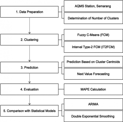
This study proposes a comprehensive forecasting framework for air quality time series data, specifically focusing on CO concentration obtained from the AQMS station in Semarang. The methodological flow, as illustrated in Figure 1, comprises five main stages: data preparation, clustering using FCM and IT2FCM, prediction based on cluster centroids, evaluation through MAPE, and comparison with traditional statistical models such as ARIMA and Double Exponential Smoothing.
3.1 Data preparation
In this stage, the collection and preparation of concentration data from the available dataset are performed. Raw data is read and structured into a matrix form suitable for clustering analysis. Subsequently, the optimal number of clusters is determined; in this study, the number of clusters is set as c=3.
The optimal number of clusters was determined not empirically, but through a systematic sensitivity analysis aimed at identifying the parameter that minimizes the Mean Absolute Percentage Error (MAPE) as detailed in Section 3.3.
Figure 1. Research methodology
3.2 Clustering
This stage involves data clustering using two methods: FCM and IT2FCM.
3.2.1 FCM
FCM is a fuzzy clustering method optimizing the following objective function (1).
$J_m(U, V)=\sum_{i=1}^n \sum_{j=1}^c\left(U_{i j}\right)^m| | x_i-v_j| |^2$ (1)
where, $U_{i j}$ represents the membership degree of data point $x_k$ to cluster $i, v_j$ denotes the centroid of cluster $j, c$ is the number of clusters, and $m$ is the fuzziness parameter, with $\mathrm{m}>1$ in this study.
3.2.2 IT2FCM
IT2FCM extends the FCM concept by incorporating two fuzziness parameters, lower m₁ and upper m2, to handle high uncertainty in data. While its objective function is conceptually similar to that of FCM, the core of the IT2FCM algorithm lies in its handling of uncertainty through type-reduction. The objective function can be expressed as:
$J_{m 1, m 2}\left(U_L, U_U, V_L, V_U\right)=\sum_{i=1}^n \sum_{j=1}^c\left[\left(U_{L i j}\right)^{m 1}| | x_i-v_{L j}| |^2+\left(U_{U i j}\right)^{m 2}| | x_i-v_{U j}| |^2\right]$ (2)
where, $U_{L i j}$, $U_{U i j}$ are respectively the lower and upper membership degrees for data $x_i$ and $v_{L j}$, $v_{U j}$ are the lower and upper centroids of cluster $j$. It is critical to note that the centroids $v_{L j}$ and $v_{U j}$ are not optimized independently. Instead, they are computed through an iterative type-reduction process, which is a hallmark of type-2 fuzzy systems. This study employs an approach aligned with established literature, where the typereduced centroid for each cluster is first calculated, and then the lower and upper centroids ($v_{L j}$ and $v_{U j}$) are derived from this type-reduced set. Algorithms such as the Karnik-Mendel (KM) algorithm are standard methods for performing this typereduction [48]. This ensures that the centroids properly reflect the footprint of uncertainty modelled by the interval memberships, rather than being simple independent optimizations.
This study set the fuzzifier parameter $\mathrm{m}=2.0$ for standard FCM, aligning with common practice and its robustness to noise in real-world datasets [49, 50]. Following the sensitivity analysis described in Section 3.3, the optimal fuzziness parameters were identified as $\mathrm{m}_1$ and $\mathrm{m}_2$. This interval, in conjunction with c clusters, was proven to provide the lowest prediction error, offering a refined balance between model sensitivity and robustness against data uncertainty.
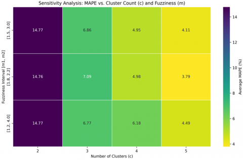
3.3 Sensitivity analysis for parameter optimization
To ensure the robustness and optimal performance of the proposed model, and in response to reviewer feedback, a sensitivity analysis was conducted. This process involved systematically evaluating the model's performance across a range of key parameters: the number of clusters (c) and the fuzziness interval [m₁, m₂]. The number of clusters c was varied from 2 to 5. The fuzziness interval was tested with three different configurations representing distinct uncertainty footprints: [1.5, 3.0], [1.8, 2.2], and [1.2, 4.0]. The model's performance for each parameter combination was measured using MAPE. This systematic approach allows for the data-driven selection of optimal parameters, moving beyond empirical estimation and enhancing the model's credibility. The results of this analysis are visualized in the heatmap in Figure 2.
Figure 2. Sensitivity analysis
3.4 Prediction
The prediction process is conducted based on the cluster centroids obtained from the previous clustering results. The predicted value $\widehat{x}_l$ for each data point is computed using the centroid of the cluster with the highest membership degree in function (3).
$\left(\widehat{x_l}\right)=v_j, j=\arg \max _j\left(U_{i j}\right)$ (3)
where, $v_j$ is the centroid of the cluster having the highest membership degree for data point $x_i$. Furthermore, the prediction mechanism is a centroid-based forecasting model that establishes a temporal link between consecutive data points via cluster membership. The process for forecasting the value at time $t+1$ based on the observation at time $t$ is as follows:
This can be formally expressed as: Let $C\left(x_t\right)$ be the cluster assigned to observation $x_t$. Then the forecast is $\hat{x}_t+1=v C_{(x t)}$. This approach effectively treats the cluster centroids as representative states of the system. The forecast is based on the assumption that the system will persist in its current state, represented by its cluster centroid, into the next time step. For the IT2FCM model, the final forecast $\hat{x}_t+1$ is the average of the lower and upper centroids for the assigned cluster, i.e., $\frac{\left(v_{L, C_{(x t)}}+v_{U, C\left(x_t\right)}\right)}{2}$.
3.5 Evaluation
Prediction performance evaluation is conducted using MAPE, computed with the Eq. (4). A lower MAPE indicates better prediction accuracy.
$M A P E=\frac{1}{n} \sum_{i=1}^n \left\lvert\, \frac{x_i-\widehat{x_l}}{x_i} \times 100 \%\right.$ (4)
3.6 Comparison with statistical models
For comparison purposes, two traditional statistical methods, namely ARIMA and Double Exponential Smoothing, are employed.
3.6.1 ARIMA
The ARIMA model is formulated in Eq. (5) with parameters $p$, $d$, $q$ representing autoregressive order, differencing, and moving average order, respectively. This study selected parameters $p, d, q$ for ARIMA via a combination of stationarity tests and inspection of ACF/PACF plots. A grid search over $\mathrm{p}=0-5$, $\mathrm{~d}=0-2$, $\mathrm{q}=0-5$ was conducted to find the model with the lowest AIC; ARIMA (2,1,2) was chosen. Additionally performed residual diagnostics to ensure model adequacy. We also tested auto arima() in pmdarima, confirming similar parameter ranges and AIC values.
$\operatorname{ARIMA}(p, d, q): y_t=c+\sum_{i=1}^p \phi_i y_{t-i}+\sum_{j=1}^q \theta_j \in_{t-j}+\in_t$ (5)
3.6.2 Double Exponential Smoothing
Double Exponential Smoothing is a time series forecasting method that addresses the limitation of simple exponential smoothing by incorporating a trend component. It uses two equations to update both the level and the trend in Eq. (6).
$\begin{aligned} & \hat{y}_t=\alpha y_t+(1-\alpha)\left(\hat{y}_{t-1}+\hat{b}_{t-1}\right) \\ & b_t=\beta\left(\hat{y}_t-\hat{y}_{t-1}\right)+(1-\beta) b_{t-1}\end{aligned}$ (6)
DES parameters $\alpha$ and $\beta$ were tuned via grid search ($\alpha$, $\beta$ $\in$[0.1,0.9]) to minimize MAPE on training data, resulting in $\alpha=0.35$ and $\beta=0.15$. This study further verified that a parameter estimation routine in Statsmodels yielded comparable values, optimizing via log-likelihood, where is the smoothing parameter for the level, and is the smoothing parameter for the trend component [51]. This method improves adaptability to trends but still assumes linearity and may struggle in volatile environments typical of sensorbased pollution monitoring.
4.1 Data source
The dataset used in this study was obtained from the AQMS Station in Mijen, Semarang City, through the official portal of the Ministry of Environment and Forestry (KLHK), Indonesia. The selected parameter is the ambient concentration of CO. The data was retrieved on 19 July 2022 and served as the input for fuzzy-based clustering and subsequent CO concentration prediction.
4.2 Clustering result
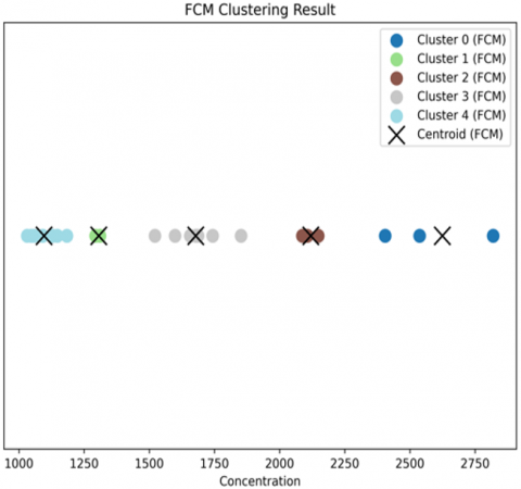
Following the parameter optimization from the sensitivity analysis, the clustering process was conducted using the optimal parameters: 5 clusters (c=5), and a fuzziness interval of [1.8, 2.2] for IT2FCM. Figure 3 presents the updated clustering results.
Figure 3(a) shows the output of the standard FCM method, which now partitions the CO concentration data into five distinct clusters. This finer granulation suggests the model has identified more nuanced concentration levels beyond a simple low-medium-high structure.
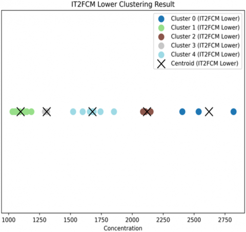
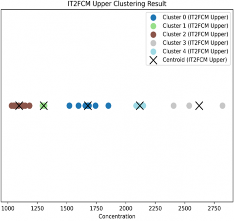
Figures 3(b) and 3(c) depict the results for the IT2FCM method, using the optimized lower and upper fuzziness parameters. Figure 3(b) (Lower Membership) and Figure 3(c) (Upper Membership) both illustrate the five-cluster structure. The subtle shifts in data point assignments and centroid positions between the lower and upper bounds demonstrate IT2FCM's capacity to robustly model the inherent uncertainty within the data, even with a more constrained fuzziness interval. This five-cluster partition forms the basis for the improved forecasting accuracy.
(a) FCM clustering result
(b) IT2FCM lower clustering result
(c) IT2FCM upper clustering result
Figure 3. IT2FCM clustering result
To provide quantitative insights into the clustering results, Tables 1-7 present the membership degrees and centroid values for each method. With the optimal parameter settings, the data points were assigned to five clusters with varying degrees of membership in Table 1, while the corresponding cluster labels are listed in Table 2. The centroid values obtained from FCM are shown in Table 3, with centroids located approximately at 2623.99, 1306.40, 2119.22, 1678.21 and 1096.26, respectively. These centroids reflect the grouping of low, medium, and high carbon monoxide concentrations.
Table 1. FCM membership
|
Data |
C1 |
C2 |
C3 |
C4 |
C5 |
|
A1 |
0.00362 |
0.00116 |
0.99076 |
0.00372 |
0.00074 |
|
A2 |
0.03113 |
0.06232 |
0.25980 |
0.61426 |
0.03248 |
|
A3 |
0.00048 |
0.00363 |
0.00209 |
0.99238 |
0.00142 |
|
A4 |
0.00530 |
0.06501 |
0.02057 |
0.88710 |
0.02202 |
|
A5 |
0.00000 |
0.00000 |
0.00000 |
0.99999 |
0.00000 |
|
A6 |
0.00009 |
0.00053 |
0.00041 |
0.99875 |
0.00022 |
|
A7 |
0.00065 |
0.00027 |
0.99795 |
0.00095 |
0.00017 |
|
A8 |
0.88003 |
0.01463 |
0.06835 |
0.02572 |
0.01128 |
|
A9 |
0.94140 |
0.00470 |
0.04081 |
0.00966 |
0.00343 |
|
A10 |
0.00507 |
0.02064 |
0.02779 |
0.93710 |
0.00940 |
|
A11 |
0.00001 |
0.99934 |
0.00003 |
0.00016 |
0.00046 |
|
A12 |
0.00046 |
0.03278 |
0.00105 |
0.00342 |
0.96229 |
|
A13 |
0.00152 |
0.05126 |
0.00327 |
0.00924 |
0.93471 |
|
A14 |
0.00093 |
0.03450 |
0.00202 |
0.00583 |
0.95672 |
|
A15 |
0.00058 |
0.02305 |
0.00126 |
0.00370 |
0.97142 |
|
A16 |
0.00049 |
0.03511 |
0.00112 |
0.00364 |
0.95965 |
|
A17 |
0.00238 |
0.32985 |
0.00565 |
0.02023 |
0.64189 |
|
A18 |
0.00001 |
0.00060 |
0.00003 |
0.00008 |
0.99929 |
|
A19 |
0.00106 |
0.09093 |
0.00244 |
0.00819 |
0.89738 |
|
A20 |
0.00009 |
0.99474 |
0.00022 |
0.00104 |
0.00391 |
|
A21 |
0.01150 |
0.30030 |
0.03914 |
0.57205 |
0.07701 |
|
A22 |
0.00356 |
0.00168 |
0.98758 |
0.00614 |
0.00104 |
|
A23 |
0.57284 |
0.02276 |
0.33636 |
0.05200 |
0.01604 |
Table 2. FCM assignment cluster
|
Data |
Cluster |
Data |
Cluster |
Data |
Cluster |
|
A1 |
3 |
A9 |
1 |
A17 |
5 |
|
A2 |
4 |
A10 |
4 |
A18 |
5 |
|
A3 |
4 |
A11 |
2 |
A19 |
5 |
|
A4 |
4 |
A12 |
5 |
A20 |
2 |
|
A5 |
4 |
A13 |
5 |
A21 |
4 |
|
A6 |
4 |
A14 |
5 |
A22 |
3 |
|
A7 |
3 |
A15 |
5 |
A23 |
1 |
|
A8 |
1 |
A16 |
5 |
Table 3. FCM centroid value
|
Cluster |
Centroid Value |
|
Cluster 1 |
2623.99 |
|
Cluster 2 |
1306.40 |
|
Cluster 3 |
2119.22 |
|
Cluster 4 |
1678.21 |
|
Cluster 5 |
1096.26 |
For the IT2FCM method, both lower and upper membership degrees are presented in Tables 4 and 5. These tables highlight how the introduction of interval fuzziness allows the same data point to have slightly different degrees of membership under varying fuzziness assumptions.
The lower and upper bound centroids in Table 6 demonstrate how IT2FCM captures uncertainty: the centroids shift slightly depending on whether a conservative (lower) or permissive (upper) fuzziness level is applied. This interval representation provides a richer characterization of the data structure, enhancing interpretability in environments with high uncertainty such as environmental pollution monitoring.
Table 4. IT2FCM lower membership
|
Data |
C1 |
C2 |
C3 |
C4 |
C5 |
|
A1 |
0.0009 |
0.0001 |
0.9978 |
0.0002 |
0.0009 |
|
A2 |
0.0168 |
0.0175 |
0.2346 |
0.0398 |
0.6913 |
|
A3 |
0.0001 |
0.0003 |
0.0005 |
0.0009 |
0.9982 |
|
A4 |
0.0016 |
0.0094 |
0.0086 |
0.0368 |
0.9436 |
|
A5 |
0.0000 |
0.0000 |
0.0000 |
0.0000 |
1.0000 |
|
A6 |
0.0000 |
0.0000 |
0.0001 |
0.0001 |
0.9998 |
|
A7 |
0.0001 |
0.0000 |
0.9997 |
0.0000 |
0.0002 |
|
A8 |
0.9377 |
0.0042 |
0.0403 |
0.0059 |
0.0119 |
|
A9 |
0.9778 |
0.0008 |
0.0174 |
0.0012 |
0.0029 |
|
A10 |
0.0014 |
0.0031 |
0.0119 |
0.0083 |
0.9753 |
|
A11 |
0.0000 |
0.0000 |
0.0000 |
1.0000 |
0.0000 |
|
A12 |
0.0001 |
0.9862 |
0.0002 |
0.0128 |
0.0008 |
|
A13 |
0.0003 |
0.9691 |
0.0009 |
0.0266 |
0.0032 |
|
A14 |
0.0002 |
0.9814 |
0.0005 |
0.0162 |
0.0018 |
|
A15 |
0.0001 |
0.9888 |
0.0003 |
0.0098 |
0.0010 |
|
A16 |
0.0001 |
0.9849 |
0.0002 |
0.0140 |
0.0008 |
|
A17 |
0.0006 |
0.7037 |
0.0018 |
0.2849 |
0.0090 |
|
A18 |
0.0000 |
0.9998 |
0.0000 |
0.0002 |
0.0000 |
|
A19 |
0.0002 |
0.9473 |
0.0006 |
0.0495 |
0.0025 |
|
A20 |
0.0000 |
0.0014 |
0.0000 |
0.9983 |
0.0003 |
|
A21 |
0.0048 |
0.0521 |
0.0222 |
0.2892 |
0.6317 |
|
A22 |
0.0009 |
0.0002 |
0.9968 |
0.0004 |
0.0018 |
|
A23 |
0.6371 |
0.0070 |
0.3145 |
0.0109 |
0.0305 |
Table 5. IT2FCM upper membership
|
Data |
C1 |
C2 |
C3 |
C4 |
C5 |
|
A1 |
0.00979 |
0.00369 |
0.00255 |
0.00968 |
0.97429 |
|
A2 |
0.55258 |
0.08177 |
0.04763 |
0.04636 |
0.27167 |
|
A3 |
0.97949 |
0.00898 |
0.00412 |
0.00168 |
0.00573 |
|
A4 |
0.82295 |
0.09214 |
0.03759 |
0.01156 |
0.03576 |
|
A5 |
0.99989 |
0.00004 |
0.00002 |
0.00001 |
0.00003 |
|
A6 |
0.99523 |
0.00189 |
0.00091 |
0.00043 |
0.00155 |
|
A7 |
0.00267 |
0.00094 |
0.00064 |
0.00196 |
0.99380 |
|
A8 |
0.04361 |
0.02720 |
0.02192 |
0.80901 |
0.09826 |
|
A9 |
0.01878 |
0.01029 |
0.00792 |
0.90083 |
0.06218 |
|
A10 |
0.88515 |
0.03669 |
0.01912 |
0.01152 |
0.04752 |
|
A11 |
0.00112 |
0.99572 |
0.00272 |
0.00013 |
0.00030 |
|
A12 |
0.00893 |
0.05964 |
0.92639 |
0.00169 |
0.00335 |
|
A13 |
0.01847 |
0.07777 |
0.89186 |
0.00412 |
0.00777 |
|
A14 |
0.01265 |
0.05626 |
0.92309 |
0.00276 |
0.00524 |
|
A15 |
0.00866 |
0.04022 |
0.94573 |
0.00185 |
0.00354 |
|
A16 |
0.00936 |
0.06293 |
0.92243 |
0.00177 |
0.00351 |
|
A17 |
0.03399 |
0.35579 |
0.59274 |
0.00573 |
0.01175 |
|
A18 |
0.00026 |
0.00137 |
0.99822 |
0.00005 |
0.00010 |
|
A19 |
0.01744 |
0.13187 |
0.84114 |
0.00318 |
0.00638 |
|
A20 |
0.00255 |
0.98878 |
0.00764 |
0.00032 |
0.00071 |
|
A21 |
0.52379 |
0.30191 |
0.09794 |
0.02025 |
0.05612 |
|
A22 |
0.01337 |
0.00453 |
0.00305 |
0.00856 |
0.97048 |
|
A23 |
0.07075 |
0.03546 |
0.02651 |
0.53382 |
0.33346 |
Table 6. IT2FCM centroid value
|
Data |
Centroid Value (Lower) |
Centroid Value (Upper) |
|
Cluster 1 |
2620.35 |
1678.09 |
|
Cluster 2 |
1097.52 |
1304.74 |
|
Cluster 3 |
2119.39 |
1095.10 |
|
Cluster 4 |
1308.16 |
2621.20 |
|
Cluster 5 |
1678.45 |
2118.26 |
4.3 Prediction result
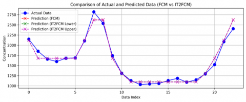
The prediction process was carried out by assigning each data point to the nearest cluster centroid and using that centroid value as the forecast. For the IT2FCM model, predictions were obtained using both lower and upper fuzziness levels. To produce a single interpretable forecast from IT2FCM, this study used the average of the two centroids, this average value reflects the central tendency of the uncertainty band modeled by IT2FCM.
Figure 4 compares the actual concentration data to the predicted values generated by FCM and IT2FCM (both lower and upper scenarios). The prediction curves closely follow the overall shape of the actual time series, with IT2FCM exhibiting improved alignment during regions of rapid fluctuation.
Figure 4. FCM and IT2FCM comparation actual data
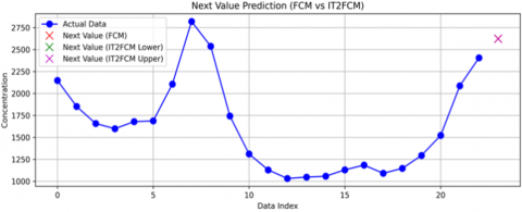
Figure 5. FCM and IT2FCM next value prediction
Figure 5 presents the next-step forecasts. The prediction from FCM was 2454.25, while IT2FCM produced a lower bound of 2374.18, an upper bound of 2464.13, and a selected average forecast of 2419.15. This average was used in subsequent comparisons for consistency.
As shown in Table 7, the use of IT2FCM-Average results in a value that is well-centered between the uncertainty bounds, providing a more stable and realistic forecast than either bound alone. This approach is particularly useful in environmental applications where short-term fluctuations and sensor noise are expected.
Table 7. MAPE and next value prediction
|
Method |
MAPE (%) |
Next Value Prediction |
|
FCM |
3.790 |
2623 |
|
IT2FCM (Lower) |
3.785 |
2620 |
|
IT2FCM (Upper) |
3.781 |
2621 |
|
IT2FCM (Average) |
3.783 |
2620 |
The quantitative evaluation using Mean Absolute Percentage Error (MAPE) supports this strategy. IT2FCM (Average) achieved a MAPE of 3.783%, which was lower than FCM (3.790%) and comparable to IT2FCM Higher (3.785%) and Upper (3.781%), as seen in the MAPE summary. These findings reinforce the use of the average value as a pragmatic balance between precision and stability.
4.4 Performance comparison with statistical models
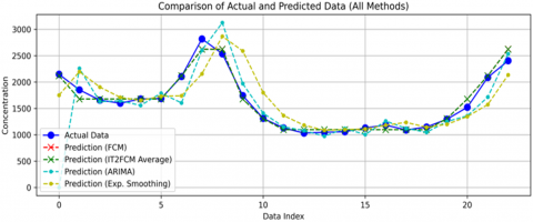
To benchmark the effectiveness of the proposed fuzzy clustering-based prediction models, two widely-used statistical forecasting methods—ARIMA and Double Exponential Smoothing—were also evaluated. Their performance was compared with FCM and IT2FCM, (average) in terms of both prediction accuracy and next value estimation. Figure 6 illustrates the actual vs. predicted concentration data for all methods.
Both FCM and IT2FCM closely follow the true data trajectory, with smoother and more stable prediction lines. In contrast, ARIMA and Double Exponential Smoothing tend to produce more erratic results, especially during abrupt changes in concentration levels. These statistical models either overreact to recent fluctuations or underrepresent rapid rises.
Figure 6. Performance comparison with statistical models
The performance metrics are summarized in the accompanying Table 8. The result is evident that IT2FCM (Average) outperforms all other methods in terms of accuracy, with a MAPE of 3.78%, significantly lower than ARIMA (13.07%) and Double Exponential Smoothing (13.75%). While FCM performs reasonably well, the added flexibility and uncertainty modeling of IT2FCM yield superior and more reliable predictions.
Table 8. Performance comparison with statistical models
|
Method |
MAPE (%) |
Next Value Prediction |
|
IT2FCM (Average) |
3.78 |
2620 |
|
ARIMA |
13.07 |
2333 |
|
Double Exp, Smoothing |
13.75 |
2455 |
The results presented in the previous sections demonstrate that the proposed fuzzy clustering-based forecasting approach—especially the IT2FCM—offers notable advantages over conventional statistical models for short-term prediction of CO concentration levels.
The first key finding is that IT2FCM consistently outperformed both FCM and baseline statistical methods (ARIMA, Exponential Smoothing) in terms of accuracy. This is evident from the MAPE, where the optimized IT2FCM (Average) model achieved a significantly lower MAPE of 3.79%. This result is not just a marginal improvement but a substantial leap in accuracy, with a prediction error less than one-third of that produced by traditional models like ARIMA (13.07%) and Exponential Smoothing (13.75%). These improvements validate the hypothesis that fuzzy clustering methods can more effectively model environmental data, which is often noisy, overlapping, and uncertain [52, 53].
Secondly, the use of interval modeling in IT2FCM introduces flexibility by capturing a range of potential centroid rather than a single point estimate. This design aligns well with real-world air quality monitoring, where variability is common, due to sensor noise, atmospheric conditions, and temporal patterns. By averaging the lower and upper bounds of IT2FCM centroids, the model yields a prediction that is both stable and interpretable, bridging precision and caution—essential in applications involving public health or environmental alerts [54].
A crucial contribution of this revised study is the inclusion of a sensitivity analysis, which addresses the parameter selection limitations of the initial approach. This analysis revealed that increasing the number of clusters from 3 to 5 allows the model to capture more granular patterns in the CO concentration data, likely corresponding to more nuanced states of air quality (e.g., very low, low, medium, high, very high). Similarly, the optimal fuzziness interval of [1.8, 2.2] demonstrates that a more constrained, moderate uncertainty footprint yields better results for this specific dataset compared to wider intervals. This data-driven parameter tuning not only validates the chosen parameters but also enhances the robustness and credibility of the proposed forecasting model.
A particularly insightful contribution is the use of the centroid-based prediction mechanism, which differs from traditional regression-based forecasting [55]. This lightweight mechanism avoids overfitting [56], ensures fast computation [57], and enables deployment in edge-computing scenarios such as IoT-based air quality monitoring stations [58].
A key limitation in the initial version of this study—the empirical selection of parameters—has now been directly addressed. By incorporating a systematic sensitivity analysis to optimize the number of clusters and fuzziness levels, the model's parameters are no longer based on heuristic choices but on a data-driven optimization process. This enhancement significantly strengthens the methodology's rigor. However, a remaining limitation is that the current study focuses solely on univariate prediction. Incorporating multivariate inputs (e.g., temperature, humidity, wind) could further enhance the model’s forecasting capabilities.
In summary, the IT2FCM-based approach introduces a novel direction in environmental time-series prediction by integrating fuzzy uncertainty modeling, interpretability, and computational simplicity. It represents a promising tool for smart environmental monitoring systems and offers potential integration into early warning platforms.
Future enhancements of the proposed IT2FCM model could include the use of multivariate input features, such as incorporating auxiliary environmental parameters (e.g., temperature, wind speed, humidity) to better capture the dynamic dependencies influencing pollutant concentration. Additionally, integrating adaptive clustering mechanisms—such as using validity indices or data-driven cluster evolution—could allow the model to adjust the number of clusters in response to non-stationary changes in environmental patterns. These improvements could significantly increase the model’s predictive robustness and operational flexibility in dynamic IoT deployments.
This study proposed a centroid-based forecasting approach for predicting ambient CO concentrations using FCM and IT2FCM clustering methods. The model was designed to handle uncertainty and overlapping patterns commonly found in environmental sensor data by leveraging fuzzy logic and interval modeling.
After performing a sensitivity analysis to identify optimal parameters (c=5, m=[1.8, 2.2]), the experimental results demonstrated the profound superiority of the proposed approach. The optimized IT2FCM (Average) model achieved the lowest MAPE at just 3.78%. This result is not only a significant improvement over the standard FCM model (3.79%) but represents a different class of accuracy compared to the traditional statistical models, ARIMA (13.07%) and Double Exponential Smoothing (13.75%). The findings strongly confirm that a data-driven, optimized IT2FCM model offers a far more accurate and reliable method for forecasting in complex environmental scenarios.
In future work to implement IT2‑FCM in microcontroller devices, measure execution time, memory usage, and power draw, and compare performance to ARIMA and DES models under identical conditions. Additionally, we will explore implementation optimizations — including memory-efficient representation and simplified fuzzification — to enable real-time uncertainty-aware forecasting on resource-constrained hardware. In future work to implement IT2‑FCM in microcontroller devices, measure execution time, memory usage, and power draw, and compare performance to ARIMA and DES models under identical conditions. Additionally, we will explore implementation optimizations—including memory-efficient representation and simplified fuzzification—to enable real-time uncertainty-aware forecasting on resource-constrained hardware.
Overall, the integration of IT2FCM clustering with a centroid-based prediction mechanism presents a promising, interpretable, and accurate approach to real-time environmental forecasting.
[1] Aswatha, S., Deepika, R., Piraba, M.D., Dhaneesh, V.P., et al. (2023). Smart air pollution monitoring system. Global Nest Journal, 25(3): 125-129. https://doi.org/10.30955/gnj.004396
[2] West, J.J., Osnaya, P., Laguna, I., Martínez, J., Fernández, A. (2004). Co-control of urban air pollutants and greenhouse gases in Mexico City. Environmental Science & Technology, 38(13): 3474-3481. https://doi.org/10.1021/es034716g
[3] Kim, H.H., Choi, S. (2018). Therapeutic aspects of carbon monoxide in cardiovascular disease. International Journal of Molecular Sciences, 19(8): 2381. https://doi.org/10.3390/ijms19082381
[4] Durante, W., Johnson, F.K., Johnson, R.A. (2006). Role of carbon monxide in cardiovascular function. Journal of Cellular and Molecular Medicine, 10(3): 672-686. https://doi.org/10.1111/j.1582-4934.2006.tb00427.x
[5] Liu, C., Yin, P., Chen, R., Meng, X., et al. (2018). Ambient carbon monoxide and cardiovascular mortality: A nationwide time-series analysis in 272 cities in China. The Lancet Planetary Health, 2(1): e12-e18. https://doi.org/10.1016/S2542-5196(17)30181-X
[6] Sitorus, R.J., Purba, I.G., Natalia, M., Tantrakarnapa, K. (2021). The effect of smoking and respiration of carbon monoxide among active smokers in Palembang. Indonesia. Kesmas, 16(2): 108-112. https://doi.org/10.21109/KESMAS.V16I2.3297
[7] Suglharto, W.H., Riadi, A.A., Ghozali, M.I. (2018). Web based information system of carbon monoxide pollution. E3S Web of Conferences, 73: 05026. https://doi.org/10.1051/e3sconf/20187305026
[8] Romero-Ávila, D., Omay, T. (2023). A long-run convergence analysis of aerosol precursors, reactive gases, and aerosols in the BRICS and Indonesia: Is a global emissions abatement agenda supported? Environmental Science and Pollution Research, 30(6): 15722-15739. https://doi.org/10.1007/s11356-022-22988-9
[9] Sugiharto, W.H., Susanto, H., Prasetijo, A.B. (2024). Selecting IoT-enabled Water Quality Index parameters for smart environmental management. Instrumentation Mesure Métrologie, 23(4): 253-263. https://doi.org/10.18280/i2m.230401
[10] Mahendra, H.N., Mallikarjunaswamy, S., Kumar, D.M., Kumari, S., Kashyap, S., Fulwani, S., Chatterjee, A. (2023). Assessment and prediction of air quality level using ARIMA model: A case study of Surat City, Gujarat State, India. Nature Environment & Pollution Technology, 22(1): 199-210. https://doi.org/10.46488/NEPT.2023.V22I01.018
[11] Bhosale, A., Chaudhari, K., Andhe, K., Naik, F., Chaudhari, S. (2023). Analysis of air pollutants affecting the air quality using ARIMA. International Research Journal of Engineering and Technology, 10(4): 585-590.
[12] Hansun, S., Wicaksana, A., Kristanda, M.B. (2021). Prediction of Jakarta City air quality index: Modified Double Exponential Smoothing approaches. International Journal of Innovative Computing, Information and Control, 17(4): 1363-1371. https://doi.org/10.24507/ijicic.17.04.1363
[13] Zhu, J., Zhang, R., Fu, B., Jin, R. (2015). Comparison of ARIMA model and exponential smoothing model on 2014 air quality index in Yanqing County, Beijing, China. Applied and Computational Mathematics, 4(6): 456-461. https://doi.org/10.11648/j.acm.20150406.19
[14] Basri, Z.A., Mohamad, N. (2018). A new hybrid of fuzzy C-Means method and fuzzy linear regression model in predicting manufacturing income. International Journal of Engineering & Technology, 7: 474-476. https://doi.org/10.14419/ijet.v7i4.30.22371
[15] Yang, B., Xu, K., Liu, Z. (2021). Fuzzy constrained inversion of magnetotelluric data using guided fuzzy C-Means clustering. Surveys in Geophysics, 42(2): 399-425. https://doi.org/10.1007/s10712-020-09628-y
[16] Mukhopadhaya, S., Kumar, A., Stein, A. (2018). FCM approach of similarity and dissimilarity measures with α-cut for handling mixed pixels. Remote Sensing, 10(11): 1707. https://doi.org/10.3390/rs10111707
[17] Ecer, F. (2022). Multi-criteria decision making for green supplier selection using interval type-2 fuzzy AHP: A case study of a home appliance manufacturer. Operational Research, 22(1): 199-233. https://doi.org/10.1007/s12351-020-00552-y
[18] Mai, D.S., Bui, K.T.T., Van Doan, C. (2023). Application of interval type-2 fuzzy logic system and ant colony optimization for hydropower dams displacement forecasting. International Journal of Fuzzy Systems, 25(5): 2052-2066. https://doi.org/10.1007/s40815-022-01452-3
[19] Yatak, M.Ö., Şahin, F. (2021). Ride comfort-road holding trade-off improvement of full vehicle active suspension system by interval type-2 fuzzy control. Engineering Science and Technology, an International Journal, 24(1): 259-270. https://doi.org/10.1016/j.jestch.2020.10.006
[20] Zheng, J., Du, W., Nascu, I., Zhu, Y., Zhong, W. (2020). An interval type-2 fuzzy controller based on data-driven parameters extraction for cement calciner process. IEEE Access, 8: 61775-61789. https://doi.org/10.1109/ACCESS.2020.2983476
[21] Chakraborty, S., Mali, K. (2022). Fuzzy and elitist cuckoo search based microscopic image segmentation approach. Applied Soft Computing, 130: 109671. https://doi.org/10.1016/j.asoc.2022.109671
[22] Najariyan, M., Qiu, L. (2021). Interval type-2 fuzzy differential equations and stability. IEEE Transactions on Fuzzy Systems, 30(8): 2915-2929. https://doi.org/10.1109/TFUZZ.2021.3097810.
[23] Sugiharto, W.H., Susanto, H., Prasetijo, A.B. (2023). Real-time water quality assessment via IoT: Monitoring pH, TDS, temperature, and turbidity. Ingénierie des Systèmes d’Information, 28(4): 823-831. https://doi.org/10.18280/isi.280403
[24] Chen, L., Lu, X. (2018). Making deep learning models transparent. Journal of Medical Artificial Intelligence. https://doi.org/10.21037/jmai.2018.07.01
[25] Ismail Fawaz, H., Forestier, G., Weber, J., Idoumghar, L., Muller, P.A. (2019). Deep learning for time series classification: A review. Data Mining and Knowledge Discovery, 33(4): 917-963. https://doi.org/10.1007/s10618-019-00619-1.
[26] Gkountakou, F.I., Papadopoulos, B.K. (2022). The use of fuzzy linear regression with trapezoidal fuzzy numbers to predict the compressive strength of lightweight foamed concrete. Mathematical Modelling of Engineering Problems, 9(1): 1-10. https://doi.org/10.18280/mmep.090101
[27] Hwang, H., Chun, I.Y., Shin, J. (2023). Improved test input prioritization using verification monitors with false prediction cluster centroids. Electronics, 13(1): 21. https://doi.org/10.3390/electronics13010021
[28] Hu, L., Pan, X., Tang, Z., Luo, X. (2021). A fast fuzzy clustering algorithm for complex networks via a generalized momentum method. IEEE Transactions on Fuzzy Systems, 30(9): 3473-3485. https://doi.org/10.1109/TFUZZ.2021.3117442
[29] Jiao, L., Yang, H., Liu, Z.G., Pan, Q. (2022). Interpretable fuzzy clustering using unsupervised fuzzy decision trees. Information Sciences, 611: 540-563. https://doi.org/10.1016/j.ins.2022.08.077
[30] Fu, Y.L., Liang, K.C. (2020). Fuzzy logic programming and adaptable design of medical products for the COVID-19 anti-epidemic normalization. Computer Methods and Programs in Biomedicine, 197: 105762. https://doi.org/10.1016/j.cmpb.2020.105762
[31] Yin, Y., Sheng, Y., Qin, J. (2022). Interval type-2 fuzzy C-Means forecasting model for fuzzy time series. Applied Soft Computing, 129: 109574. https://doi.org/10.1016/j.asoc.2022.109574
[32] Chen, Y., Liu, L., Cao, J., Wang, K., Li, S., Yin, Y. (2025). An enhanced interval type-2 fuzzy C-Means algorithm for fuzzy time series forecasting of vegetation dynamics: A case study from the Aksu Region, Xinjiang, China. Land, 14(6): 1242. https://doi.org/10.3390/land14061242
[33] Bhanja, S., Das, A. (2024). An air quality forecasting method using fuzzy time series with butterfly optimization algorithm. Microsystem Technologies, 30(5): 613-623. https://doi.org/10.1007/s00542-023-05591-x
[34] Pinto, A.C.V., Fernandes, T.E., Silva, P.C., Guimarães, F.G., Wagner, C., Pestana de Aguiar, E. (2022). Interval type-2 fuzzy set based time series forecasting using a data-driven partitioning approach. Evolving Systems, 13(5): 703-721. https://doi.org/10.1007/s12530-022-09452-2
[35] Shao, H., Zhang, D.Q., Lu, F. (2025). Enhanced prediction model for time series characterized by GARCH via interval type-2 fuzzy inference system. arXiv preprint arXiv:2505.01675. https://doi.org/10.48550/arXiv.2505.01675
[36] Che Mat Nor, S.M., Shaharudin, S.M., Ismail, S., Mohd Najib, S.A., Tan, M.L., Ahmad, N. (2022). Statistical modeling of RPCA-FCM in spatiotemporal rainfall patterns recognition. Atmosphere, 13(1): 145. https://doi.org/10.3390/atmos13010145
[37] Lu, W., Feng, G., Liu, X., Pedrycz, W., Zhang, L., Yang, J. (2019). Fast and effective learning for fuzzy cognitive maps: A method based on solving constrained convex optimization problems. IEEE Transactions on Fuzzy Systems, 28(11): 2958-2971. https://doi.org/10.1109/TFUZZ.2019.2946119
[38] Yang, Z., Chung, F.L., Shitong, W. (2009). Robust fuzzy clustering-based image segmentation. Applied Soft Computing, 9(1): 80-84. https://doi.org/10.1016/j.asoc.2008.03.009
[39] Huo, H., Guo, J., Li, Z.L., Jiang, X. (2017). Remote sensing of spatiotemporal changes in wetland geomorphology based on type 2 fuzzy sets: A case study of Beidagang wetland from 1975 to 2015. Remote Sensing, 9(7): 683. https://doi.org/10.3390/rs9070683
[40] Rodríguez-Ramos, A., da Silva Neto, A.J., Llanes-Santiago, O. (2023). An improved fault diagnosis scheme based on a type-2 fuzzy classification algorithms. In International Workshop on Artificial Intelligence and Pattern Recognition, pp. 84-95. https://doi.org/10.1007/978-3-031-49552-6_8
[41] Du, Y., Lu, X., Zeng, W., Hu, C. (2016). Interval type-2 fuzzy linear discriminant analysis for gender recognition. In Biometric Recognition: 11th Chinese Conference, Chengdu, China, pp. 195-202. https://doi.org/10.1007/978-3-319-46654-5_22
[42] Castillo, O., Castro, J.R., Melin, P. (2022). Interval type-3 fuzzy aggregation of neural networks for multiple time series prediction: The case of financial forecasting. Axioms, 11(6): 251. https://doi.org/10.3390/axioms11060251
[43] Sarkodie, S.A. (2017). Estimating Ghana’s electricity consumption by 2030: An ARIMA forecast. Energy Sources, Part B: Economics, Planning, and Policy, 12(10): 936-944. https://doi.org/10.1080/15567249.2017.1327993
[44] Jafridin, M.A., Fauzi, N.F., Alias, R., Ab Halim, H.Z., Bakhtiar, N.S.A., Khairudin, N.I., Shafii, N.H. (2021). A comparison of fuzzy time series and ARIMA to forecast tourist arrivals to homestay in Pahang. Journal of Computing Research and Innovation, 6(4): 83-92. https://doi.org/10.24191/jcrinn.v6i4.235
[45] Udenio, M., Vatamidou, E., Fransoo, J.C. (2023). Exponential smoothing forecasts: Taming the bullwhip effect when demand is seasonal. International Journal of Production Research, 61(6): 1796-1813. https://doi.org/10.1080/00207543.2022.2048114
[46] Sano, H., Yamada, K. (2021). Prediction accuracy of sales surprise for inventory turnover. International Journal of Production Research, 59(17): 5337-5351. https://doi.org/10.1080/00207543.2020.1778205
[47] Sadeghi, A. (2015). Providing a measure for bullwhip effect in a two-product supply chain with exponential smoothing forecasts. International Journal of Production Economics, 169: 44-54. https://doi.org/10.1016/j.ijpe.2015.07.012
[48] Karnik, N.N., Mendel, J.M. (2001). Operations on type-2 fuzzy sets. Fuzzy Sets and Systems, 122(2): 327-348. https://doi.org/10.1016/S0165-0114(00)00079-8
[49] Wu, K.L. (2012). Analysis of parameter selections for fuzzy C-Means. Pattern Recognition, 45(1): 407-415. https://doi.org/10.1016/j.patcog.2011.07.012
[50] Huang, M., Xia, Z., Wang, H., Zeng, Q., Wang, Q. (2012). The range of the value for the fuzzifier of the fuzzy C-Means algorithm. Pattern Recognition Letters, 33(16): 2280-2284. https://doi.org/10.1016/j.patrec.2012.08.014
[51] Parasian, S., Hidayatulah, H., Romanus, D. (2020). Forecasting acceptance of new students using Double Exponential Smoothing method. Journal of Critical Review, 7(1): 300-305. https://doi.org/10.31838/jcr.07.01.57
[52] Riaz, S., Arshad, A., Jiao, L. (2018). Fuzzy rough C-Mean based unsupervised CNN clustering for large-scale image data. Applied Sciences, 8(10): 1869. https://doi.org/10.3390/app8101869
[53] Shen, Y., Pedrycz, W., Chen, Y., Wang, X., Gacek, A. (2019). Hyperplane division in fuzzy C-Means: Clustering big data. IEEE Transactions on Fuzzy Systems, 28(11): 3032-3046. https://doi.org/10.1109/TFUZZ.2019.2947231
[54] Tarafdar, A., Majumder, P., Bera, U.K. (2023). Prediction of air quality index in Kolkata city using an advanced learned interval type-3 fuzzy logic system. In 2023 IEEE 8th International Conference for Convergence in Technology (I2CT), Lonavla, India, pp. 1-7. https://doi.org/10.1109/I2CT57861.2023.10126430
[55] Gong, Y., Xiang, L., Liu, G. (2020). Fuzzy regression model based on geometric centroid and incentre points and application to performance evaluation. International Journal of Uncertainty, Fuzziness and Knowledge-Based Systems, 28(2): 269-288. https://doi.org/10.1142/S0218488520500117
[56] Li, Y., Chen, X., Rao, P., Zhang, S., Liu, G. (2024). A resolution and localization algorithm for closely-spaced objects based on improved YOLOv5 joint fuzzy C-Means clustering. IEEE Photonics Journal, 16(4): 1-13. https://doi.org/10.1109/JPHOT.2024.3361433
[57] Yuwono, M., Su, S.W., Moulton, B., Nguyen, H. (2012). Method for increasing the computation speed of an unsupervised learning approach for data clustering. In 2012 IEEE Congress on Evolutionary Computation, Brisbane, QLD, Australia, pp. 1-8. https://doi.org/10.1109/CEC.2012.6252927
[58] Liang, Q. (2010). Situation understanding based on heterogeneous sensor networks and human-inspired favor weak fuzzy logic system. IEEE Systems Journal, 5(2): 156-163. https://doi.org/10.1109/JSYST.2010.2090404