Ali Alilouche*![]() | Rédha Bendoumia
| Rédha Bendoumia![]() | Islam Hassani
| Islam Hassani![]() | Felix Albu
| Felix Albu![]()
© 2025 The authors. This article is published by IIETA and is licensed under the CC BY 4.0 license (http://creativecommons.org/licenses/by/4.0/).
OPEN ACCESS
This paper presents a modified algorithm for addressing acoustic impulse responses identification for communication systems. This study introduces an enhanced sub-band version of variable-step-size µ-law proportionate normalized least-mean-square algorithm for achieving rapid convergence and minimal steady-state error. This algorithm is noted as SPV-NLMS: Sub-band Proportionate Variables-step-sizes NLMS algorithm. The proposed SPV-NLMS algorithm is dynamically and independently adjusting the N step-sizes parameters during adaptation using an optimal estimation of each sub-filter. The SPV-NLMS is adaptable and can be employed with various acoustic more dispersive, dispersive, more sparse or sparse environments. The effectiveness of this algorithm is validated through simulations in the context of acoustic impulse response identification. The SPV-NLMS algorithm has the potential to significantly improve the convergence and the steady-state error using the Mean Square Error (MSE) and Echo Return Loss Enhancement (ERLE) criteria.
acoustical system identification, adaptive sub-filter, dispersive and sparse impulse response, proportionate NLMS algorithm, variable-step-size
Digital signal processing is a very important field on communication systems, enabling smooth information exchange across vast distances and diverse environments, serving as the foundation of our interconnected world. Adaptive signal processing, noise reduction and echo cancellation are crucial for the efficiency and reliability of modern communication systems [1]. They involve processing and analyzing signals to extract useful information from noisy environments, leading to enhanced data transmission and reception [2]. Advanced adaptive filtering algorithms used in communication, such as acoustic system identification [3] and beamforming [4, 5], allow systems to adapt in changing channel conditions, ensuring continuous connectivity.
Acoustic impulse response identification is a fundamental aspect of adaptive filtering algorithms, which is integrated to diverse fields like telecommunications, audio engineering, and control systems [6-8]. The Least Mean Squares (LMS) and its normalized version (NLMS), utilize input signals and desired outputs to estimate the acoustical impulse response of a system [6]. By iteratively adjusting filter coefficients, the algorithm minimizes the error between predicted and actual outputs. This process allows us to adapt to changing environments in real-time, making it incredibly useful for applications like echo cancellation in telephony and reducing noise in audio processing. Identifying impulse responses using adaptive filtering enables systems to accurately capture the dynamic behavior of complex systems, leading to improved performance, improved signal quality, and more accurate responses in cases of varying conditions [9-11]. The basic proportionate NLMS algorithm and its variants are used in sparse impulse response identification applications [12-15]. To improve the convergence rate, the sub-band decomposition is very useful, but the final steady-state error is large [16-19]. To solve this problem, the addition of a variable step size parameter is crucial [20, 21].
In this paper, we propose a new sub-band implementation of the proportionate variable-step-sizes NLMS algorithm. The utilization of the µ-law compression in the PNLMS algorithm allows for enhanced handling of signals with varying dynamic ranges, effectively preserving the fine details while adapting to larger variations. By adopting a sub-band structure, the algorithm can segment the input signal into different frequency components, enabling precise adaptation within specific frequency ranges. Moreover, the incorporation of independent variable parameters improves the adaptability by optimal step-sizes to match the unique characteristics of each sub-band.
Section 2 presents the impulse response identification system using the basic NLMS algorithm. The new implementation of the proposed sub-band proportionate algorithm with new separated variable-step-sizes parameters, is presented and discussed in Section 3. Section 4 presents a comprehensive discussion of simulation results, incorporating diverse objective criteria that highlight the performance of the proposed SPV-NLMS algorithm. Section 5 presents the conclusion of this study.
2.1 Acoustic impulse response
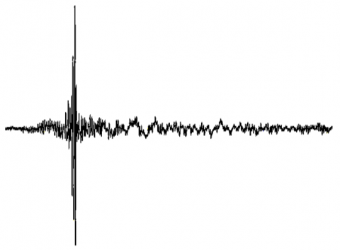
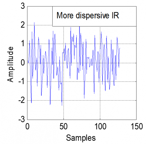
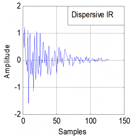
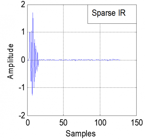
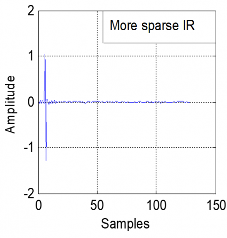
An acoustical impulse response refers to the characteristic acoustic behavior of a space or environment in response to a short impulsive sound signal. It describes how sound waves travel, reflect, and attenuate within a given space over time. The acoustical impulse response encompasses various acoustic phenomena, such as reflections, diffraction, absorption, and reverberation, which collectively shape the sound behavior within a specific location. There are two types of impulse responses in acoustical systems [22]: dispersive impulse responses and sparse impulse responses. The dispersive impulse responses are characterized by the propagation of signal components over time, resulting in a spread-out or smeared response. In such cases, the system response is influenced by frequency-dependent delays, causing diverse frequency components of the signal to arrive at diverse times. The sparse impulse responses are characterized by a relatively small number of significant response values, with most of the response values being close to zero [12]. Sparse impulse responses are often encountered in scenarios where there is a clear line-of-sight propagation path or minimal reflections [13]. In Figure 1, we present the real acoustical dispersive/sparse impulse responses.
(a)
(b)
Figure 1. Real impulse responses, (a) Dispersive, (b) Sparse [23]
2.2 Identification system process
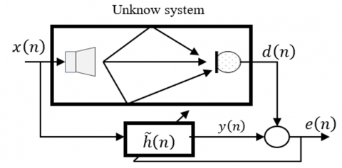
Impulse response identification is a process in signal processing where the characteristics of a system in response to an impulsive input signal are estimated [24]. The impulse response describes how a system reacts to a brief, instantaneous input, and it encompasses information about the system behavior, time delays, amplitude scaling, and filtering effects. This process is fundamental in understanding and modeling various systems, such as communication channels, audio systems, and room acoustics [25]. Figure 2 shows a basic acoustical adaptive system identification, where we note that the output desired signal $d(n)$ in the closed acoustical room is given by convoluting the input signal $x(n)$ with the acoustic impulse response $h(n)$.
$d(n)=x(n) * h(n)$ (1)
In the other hand, the adaptive filter output $y(n)$ presents as convolution among the input $x(n)$ and adaptive filter coefficients $\tilde{h}(n)$.
$y(n)=x(n) * \tilde{h}(n)$ (2)
We note that the error $e(n)$ is a crucial component in various algorithms used to adjust system parameters. The goal is to iteratively reduce this error signal, thus improving the system's performance or convergence to a desired state. Mathematically, $e(n)$ can be defined as:
$e(n)=d(n)-y(n)$ (3)
By inserting Eqs. (1) and (2) into Eq. (3), we obtain
$e(n)=x(n) * h(n)-x(n) * \tilde{h}(n)$ (4)
$e(n)=x(n) *[h(n)-\tilde{h}(n)]$ (5)
During the phase of stable convergence, the filter $\tilde{h}(n)$ achieves convergence with the room impulse response $\tilde{h}(n)=$ $h(n)$. Consequently, the computed error takes the form:
$e(n)=0$ (6)
Figure 2. Acoustical adaptive system identification [26]
2.3 Adaptive NLMS algorithm
The NLMS is a popular adaptive filtering algorithm used in various signal processing applications, including system identification. The NLMS algorithm is specifically used for identifying the dispersive impulse response.
Firstly, we note that the adaptive filter vector is defined as: $\widetilde{\boldsymbol{h}}(n)=\left[\tilde{h}_1(n), \tilde{h}_2(n), \ldots, \tilde{h}_M(n)\right]^T$, where $M$ is the length of the impulse response. We compute the estimated output $y(n)$ at iteration $n$ by taking the dot product of the current impulse response estimate and the input signal vector $x(n)$ :
$y(n)=[\tilde{\mathbf{h}}(n-1)]^T \mathbf{x}(n)$ (7)
where, $\mathbf{x}(n)=[x(n), x(n-1), \ldots, x(n-M+1)]^{\mathrm{T}}$.
The error $e(n)$ is the difference between the actual output $d(n)$ and the estimated output $y(n)$, i.e., $e(n)=d(n)-$ $y(n)$. Then the output error $e(n)$ is normalized by a normalization factor $\alpha(n)$ which is the sum of squares of the recent $M$ elements of the input signal vector $x(n)$, plus a small positive constant $\varepsilon$ to prevent division by zero is calculated:
$\alpha(n)=\mathbf{x}(n)^T \mathbf{x}(n)+\varepsilon$ (8)
The adaptation of the estimate filter $\widetilde{\boldsymbol{h}}(n)$ using the NLMS algorithm is defined by the next expression:
$\tilde{\mathbf{h}}(n)=\tilde{\mathbf{h}}(n-1)+\mu_n \frac{e(n) \mathbf{x}(n)}{\alpha(n)}$ (9)
These steps are repeated for each iteration $n=$ $1,2,3, \ldots$, end, and a stopping criterion is used. This criterion can be a maximum number of iterations or a threshold on the error $e(n)$, indicating that the algorithm has converged or the desired accuracy has been achieved. $\mu_n$ is the fixed normalized step-size parameter that has values between 0 and 2 [1-6].
For some applications [3], the length of acoustic impulse responses can be high, often ranging from 100 to 400 milliseconds and characterized by sparse impulse responses. An essential aspect is the individual adjustment of adaptation step-sizes for these sub-filters. This signifies that the variable parameter assigned to each independent sub-filter is personalized and fine-tuned autonomously in comparison to the others.
In this section, we present the proposed sub-band proportionate variable-step-sizes NLMS algorithm, noted SPV-NLMS. In SPV-NLMS, the µ-law proportionate enhances signal handling for varying dynamic ranges, preserving details while adapting to larger variations. The proposed algorithm introduces an innovative approach by employing proportionate variable step sizes specifically tailored to each individual sub-band frequency. While existing proportionate algorithms, such as PNLMS, excel in improving the convergence rate during the initial stages of adaptation, their performance significantly deteriorates thereafter. Sub-band decomposition-based algorithms, on the other hand, offer the advantage of achieving high convergence rates, particularly when input sequences exhibit strong correlation. To ensure minimal misalignment in the steady state, various variable step-size (VSS) algorithms have been developed in the literature.
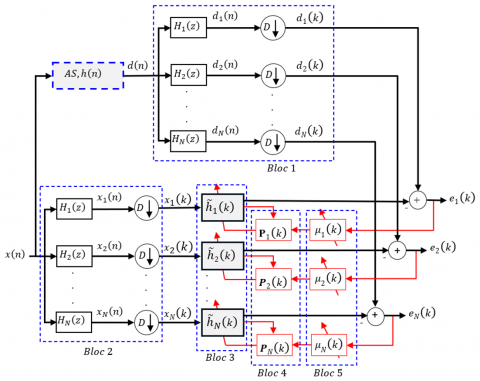
The key contribution of the proposed algorithm lies in leveraging these advantages to deliver superior performance compared to existing methods. It achieves precise adaptation across diverse frequency components, with the unique incorporation of distinct variable step-size parameters for each sub-band further enhancing the algorithm's adaptability and efficiency. The general diagram of the proposed SPV-NLMS algorithm is presented in Figure 3.
As an initial stage, as presented in Figure 3, (see two blocs 1 and 2), two analysis filter banks combined with decimation parts to partition $x(n)$ and $d(n)$ into $N$ separate frequency sub-bands are employed The decimation parts are used to down-sample the $N$-sub-signals. The process of analysis filtering involves the decomposition of the input signal into $N$. sub-bands, wherein each of these sub-bands corresponds to a distinct frequency range. Each filter is responsible for isolating a particular set of frequencies, thereby generating an array of sub-band signals. The output sub-signals of two analysis filter banks can be described as follows:
$\left\{\begin{array}{c}x_1(n)=x(n)^* h_1(n) \\ x_2(n)=x(n)^* h_2(n) \\ \vdots \\ x_N(n)=x(n) * h_N(n)\end{array}\right.$ (10)
$\left\{\begin{array}{c}d_1(n)=d(n)^* h_1(n) \\ d_2(n)=d(n)^* h_2(n) \\ \vdots \\ d_N(n)=d(n) * h_N(n)\end{array}\right.$ (11)
Each analysis filter directly relates to one of the sub-signals. The comprehensive expressions, both in general and vector form, for decomposing the input and desired sub-signals are as follows:
$x_i(n)=x(n)^* h_i(n)$ (12)
$d_i(n)=d(n) * h_i(n)$ (13)
$x_i(n)=\left[\mathbf{x}_l(n)\right]^T \mathbf{h}_i(n)$ (14)
$d_i(n)=[\mathbf{d}(n)]^T \mathbf{h}_i(n)$ (15)
with $i=1,2, \ldots, N, L$ is the length of analysis filter and:
$\begin{gathered}\mathbf{h}_i(n)=\left[h_{(i, 1)}(n), h_{(i, 2)}(n), \ldots, h_{(i, L)}(n)\right]^T, \\ \mathbf{x}_l(n)=[x(n), x(n-1), \ldots, x(n-L+1)]^T, \\ \mathbf{d}(n)=[d(n), d(n-1), \ldots, d(n-L+1)]^T .\end{gathered}$
The down-sampling factor is denoted as $D$, and it governs the extent of reduction in the sample rate, specifically $N=D$. In this process, the timing index " $n$ " is modified to " $k$ " to reflect the decimated timing. The result of this decimation applied to the input sub-signals are defined as:
$\left\{\begin{array}{c}x_1(k)=x_1(n D) \\ x_2(k)=x_2(n D) \\ \vdots \\ x_N(k)=x_N(n D)\end{array}\right.$ (16)
$\left\{\begin{array}{c}d_1(k)=d_1(n D) \\ d_2(k)=d_2(n D) \\ \vdots \\ d_N(k)=d_N(n D)\end{array}\right.$ (17)
The general formulation of the decimated input and the desired sub-signals can be presented as follows:
$x_i(k)=x_i(n D)$ (18)
$d_i(k)=d_i(n D)$ (19)
where, $x_i(n)$ represent the original input sub-signals prior to decimation, $x_i(k)$ denote the decimated input subsignals, $d_i(n)$ represent the original desired sub-signals prior to decimation, and $d_i(k)$ denote the decimated desired subsignals. Using the sub-band methodology provides an efficient adaptation procedure, leading to faster convergence rates when identifying acoustic impulse responses within long sparse environments (the third block of Figure 3).
Figure 3. The detailed scheme of the proposed adaptive algorithm for impulse response identification
All adaptation formulas of the proposed SPV-NLMS algorithm, which relies on distinct proportionate and variable-step-size parameters, are defined as follows:
$\left\{\begin{array}{c}\tilde{\boldsymbol{h}}_1(k)=\tilde{\boldsymbol{h}}_1(k-1)+\mu_1(k) \frac{\boldsymbol{P}_1(k-1) \boldsymbol{x}_1(k) e_1(k)}{\alpha_1(k)} \\ \widetilde{\boldsymbol{h}}_2(k)=\widetilde{\boldsymbol{h}}_2(k-1)+\mu_2(k) \frac{\boldsymbol{P}_2(k-1) \boldsymbol{x}_2(k) e_2(k)}{\alpha_2(k)} \\ \vdots \\ \widetilde{\boldsymbol{h}}_N(k)=\widetilde{\boldsymbol{h}}_N(k-1)+\mu_N(k) \frac{\boldsymbol{P}_N(k-1) \boldsymbol{x}_N(k) e_N(k)}{\alpha_N(k)}\end{array}\right.$ (20)
with $\alpha_1(k), \alpha_2(k), \ldots, \alpha_N(k)$ represent the modified normalization factors linked to each input sub-signals $x_1(k)$, $x_2(k), \ldots, x_N(k)$, respectively. These modified factors are given by:
$\left\{\begin{array}{c}\alpha_1(k)=\left[\mathbf{x}_1(k)\right]^T \mathbf{P}_1(k-1) \mathbf{x}_1(k)+\varepsilon \\ \alpha_2(k)=\left[\mathbf{x}_2(k)\right]^T \mathbf{P}_2(k-1) \mathbf{x}_2(k)+\varepsilon \\ \vdots \\ \alpha_N(k)=\left[\mathbf{x}_N(k)\right]^T \mathbf{P}_N(k-1) \mathbf{x}_N(k)+\varepsilon\end{array}\right.$ (21)
In this context, the M × M size matrices $\mathbf{P}_1(k-1), \mathbf{P}_2(k-$ $1), \ldots, \mathbf{P}_N(k-1)$ are used to govern the step-sizes associated with each coefficient of the individual sub-filters. $\mu_1(k)$, $\mu_2(k), \ldots, \mu_N(k)$ represent the individual variable-step-size parameters assigned respectively to the sub-filters $\tilde{\mathbf{h}}_1(k)$, $\tilde{\boldsymbol{h}}_2(k), \ldots, \tilde{\boldsymbol{h}}_N(k)$.
Next, all control diagonal matrices $\mathbf{P}_i(k-1)$ and individual variable-step-size parameters $\mu_i(k)$ that are used to ensure a rapid and efficient adaptation of all sub-filters $\widetilde{\boldsymbol{h}}_i(k)$ are detailed. The general updating equation by the proposed SPV-NLMS algorithm is given by:
$\tilde{\mathbf{h}}_i(k)=\tilde{\mathbf{h}}_i(k-1)+\mu_i(k) \frac{\mathbf{P}_i(k-1) \mathbf{x}_i(k) e_i(k)}{\alpha_i(k)}$ (22)
with, $\begin{aligned} & \tilde{\mathbf{h}}_i(k)=\left[\tilde{h}_{i, 1}(k), \tilde{h}_{i, 2}(k), \ldots, \tilde{h}_{i, M}(k)\right]^{\mathrm{T}}, \quad \mathbf{x}_i(k)=\left[x_i(k),\right. \left.x_i(k-1), \ldots, x_i(k-M+1)\right]^{\mathrm{T}}, \quad \alpha_i(k)=\left[\mathbf{x}_i(k)\right]^T \mathbf{P}_i(k- { 1) } \mathbf{x}_i(k)+\varepsilon .\end{aligned}$
Block 3 of Figure 3 presents the adaptation filters in sub-band form using N individual proportionate and variable-step-size parameters. We note that the decimated error sub-signals in the output are given by:
$\left\{\begin{array}{c}e_1(k)=d_1(k)-y_1(k) \\ e_2(k)=d_2(k)-y_2(k) \\ \vdots \\ e_N(k)=d_N(k)-y_N(k)\end{array}\right.$ (23)
The general formula for the sub-signal $y_i(k)$ of the all-output filters can be defined as:
$y_i(k)=x_i(k) * \tilde{h}_i(k)$ (24)
The general vectorial equation is the following:
$y_i(k)=\left[\mathbf{x}_i(k)\right]^T \widetilde{\mathbf{h}}_i(k)$ (25)
By substituting the last equation into Eq. (23) for estimated sub-signals, the next expressions are obtained:
$\left\{\begin{array}{c}e_1(k)=d_1(k)-\left[\mathbf{x}_1(k)\right]^T \tilde{\mathbf{h}}_1(k) \\ e_2(k)=d_2(k)-\left[\mathbf{x}_2(k)\right]^T \tilde{\mathbf{h}}_2(k) \\ \vdots \\ e_N(k)=d_N(k)-\left[\mathbf{x}_N(k)\right]^T \tilde{\mathbf{h}}_N(k)\end{array}\right.$ (26)
Considering the general equation for error sub-signals, it can be expressed as follows:
$e_i(k)=d_i(k)-\left[\mathbf{x}_i(k)\right]^T \tilde{\mathbf{h}}_i(k)$ (27)
The utilization of the proportionate adaptive algorithm proves to be particularly effective in the context of identifying sparse impulse responses (see Block 4). This adaptive filtering technique enhances the precision of signal processing tasks in scenarios where the impulse responses are sparsely distributed. The algorithm capitalizes on the inherent sparsity by assigning varying step-sizes to individual filter coefficients as presented in fourth step. Larger coefficients, which are more influential in contributing to the response, are assigned proportionately larger step-sizes. In the proportionate adaptive approach, each filter coefficient is assigned a unique step-size [14].
This means that larger coefficients are granted greater increments, resulting in an amplified convergence rate for those specific coefficients.
The µ-law compression function employed in our algorithm is instrumental in emphasizing small signal variations while compressing larger amplitudes, making it particularly effective for signals with large dynamic ranges. For larger values of $\left|\tilde{h}_{i, m}(k)\right|$, the logarithmic nature of the compression reduces the relative magnitude, mitigating the impact of dominant coefficients.
Conversely, for smaller coefficients, the compression function behaves approximately linearly, allowing for more precise adjustments. This balance ensures improved steady-state precision and enhances convergence speed, as smaller coefficients are not neglected during adaptation, and large variations are effectively controlled.
Additionally, µ-law compression inherently provides robustness to outliers and better handling of non-stationary environments, making it a critical feature for adaptive filtering algorithms in dynamic scenarios.
The values of the diagonal control matrix $\mathbf{P}_i(k)$ are determined by the following formulas:
$\left\{\begin{array}{c}\mathbf{P}_1(k)={diag}\left[p_{1,1}(k), p_{1,2}(k), \ldots, p_{1, M}(k)\right] \\ \mathbf{P}_2(k)={diag}\left[p_{2,1}(k), p_{2,2}(k), \ldots, p_{2, M}(k)\right] \\ \vdots \\ \mathbf{P}_N(k)={diag}\left[p_{N, 1}(k), p_{N, 2}(k), \ldots, p_{N, M}(k)\right]\end{array}\right.$ (28)
The diagonal elements of $\mathbf{P}_i(k)$, as represented in Eq. (28), are denoted by $p_{i, m}(k)$ with $m=1,2, \ldots, M$. These elements are determined through the following expressions:
$\left\{\begin{aligned} p_{1, m}(k)= & \frac{\gamma_{1, m}(k)}{\sum_{l=1}^M\left[\gamma_{1, l}(k)\right]} \\ p_{2, m}(k)= & \frac{\gamma_{2, m}(k)}{\sum_{l=1}^M\left[\gamma_{2, l}(k)\right]} \\ & \vdots \\ p_{N, m}(k)= & \frac{\gamma_{N, m}(k)}{\sum_{l=1}^M\left[\gamma_{N, l}(k)\right]}\end{aligned}\right.$ (29)
where, the general diagonal elements of $\mathbf{P}_i(k)$ is given by:
$p_{i, m}(k)=\frac{\gamma_{i, m}(k)}{\sum_{l=1}^M\left[\gamma_{i, l}(k)\right]}$ (30)
and
$\left\{\begin{array}{c}\gamma_{1, m}(k)={Max}\left\{\rho \times F\left(\left|\tilde{h}_{1, m}(k)\right|\right), F_{Log }\left(\left|\tilde{h}_{1, m}(k)\right|\right)\right\} \\ \gamma_{2, m}(k)={Max}\left\{\rho \times F\left(\left|\tilde{h}_{2, m}(k)\right|\right), F_{Log }\left(\left|\tilde{h}_{2, m}(k)\right|\right)\right\} \\ \vdots \\ \gamma_{N, m}(k)={Max}\left\{\rho \times F\left(\left|\tilde{h}_{N, m}(k)\right|\right), F_{Log }\left(\left|\tilde{h}_{N, m}(k)\right|\right)\right\}\end{array}\right.$ (31)
with the general formula is:
$\gamma_{i, m}(k)={Max}\left\{\rho \times F\left(\left|\tilde{h}_{i, m}(k)\right|\right), F_{{Log }}\left(\left|\tilde{h}_{i, m}(k)\right|\right)\right\}$ (32)
with $\rho=5 / M$, to prevent any inactivity during the adaptation phase.
The functions $F\left(\left|\tilde{h}_{1, m}(k)\right|\right), F\left(\left|\tilde{h}_{2, m}(k)\right|\right), \ldots, F\left(\left|\tilde{h}_{\mathrm{N}, m}(k)\right|\right)$ are given by:
$\left\{\begin{array}{l}F\left(\left|\tilde{h}_{1, m}(k)\right|\right)={Max}\left\{\begin{array}{c}\delta, F_{Log}\left(\left|\tilde{h}_{1,1}(k)\right|\right), F_{Log}\left(\left|\tilde{h}_{1,2}(k)\right|\right), \\ \ldots, F_{log }\left(\left|\tilde{h}_{1, M}(k)\right|\right) .\end{array}\right\} \\ F\left(\left|\tilde{h}_{2, m}(k)\right|\right)={Max}\left\{\begin{array}{c}\delta, F_{Log}\left(\left|\tilde{h}_{2,1}(k)\right|\right), F_{Log}\left(\left|\tilde{h}_{2,2}(k)\right|\right), \\ \ldots, F_{Log}\left(\left|\tilde{h}_{2, M}(k)\right|\right) .\end{array}\right\} \\ \vdots \\ F\left(\left|\tilde{h}_{N, m}(k)\right|\right)={Max}\left\{\begin{array}{c}\delta, F_{Log}\left(\left|\tilde{h}_{N, 1}(k)\right|\right), F_{Log}\left(\left|\tilde{h}_{N, 2}(k)\right|\right) \\ \ldots, F_{Log}\left(\left|\tilde{h}_{N, M}(k)\right|\right) .\end{array}\right\}\end{array}\right.$ (33)
The general function $F\left(\left|\tilde{h}_{\mathrm{I}, m}(k)\right|\right)$ is:
$F\left(\left|\tilde{h}_{i, m}(k)\right|\right)={Max}\left\{\begin{array}{c}\delta, F_{log }\left(\left|\tilde{h}_{i, 1}(k)\right|\right), F_{log }\left(\left|\tilde{h}_{i, 2}(k)\right|\right), \\ \ldots, F_{log }\left(\left|\tilde{h}_{i, M}(k)\right|\right)\end{array}\right\}$ (34)
where, $\delta$ is the regularization component that is typically set at 0.01, and introduces a slight non-zero value, contributing to the regulation and stabilization of the updating process. The $N$ logarithmic functions are given by:
$\left\{\begin{aligned} F_{ {Log }}\left(\left|\tilde{h}_{1, m}(k)\right|\right)= & \frac{ln \left(\mu \times\left|\tilde{h}_{1, m}(k)\right|+1\right)}{ln (\mu+1)} \\ F_{ {Log }}\left(\left|\tilde{h}_{2, m}(k)\right|\right)= & \frac{ln \left(\mu \times\left|\tilde{h}_{2, m}(k)\right|+1\right)}{ln (\mu+1)} \\ & \vdots \\ F_{ {Log }}\left(\left|\tilde{h}_{N, m}(k)\right|\right)= & \frac{ln \left(\mu \times\left|\tilde{h}_{N, m}(k)\right|+1\right)}{ln (\mu+1)}\end{aligned}\right.$ (35)
with the general logarithmic function is given by:
$F_{L o g}\left(\left|\tilde{h}_{I, m}(k)\right|\right)=\frac{ln \left(\mu \times\left|\tilde{h}_{i, m}(k)\right|+1\right)}{\ln (\mu+1)}$ (36)
The determination of the positive quantity $\mu$ depends on the noise level. For identifying sparse impulse responses, a practical selection for $\xi$ is 0.001 . Additionally, $\mu$ stands for the inverse of $\xi, \mu=1 / \xi$.
An important contribution presented in Block 5 is the distinct optimal step-size relationships designed for faster convergence and very low error. In adaptive filtering, the significance of the step-size lies in its efficient role during updates of coefficients. Our focus in optimizing these distinct step-size parameters is dual: enhancing the convergence rate and lessening the difference between desired various impulse responses and both estimated and actual impulse responses. It's significant that our primary attention centers on $N$ error sub-signals, denoted as $e_i(k)$, which derive from the process of adaptive sub-filtering. We define $\boldsymbol{\epsilon}_i(k)$ as weight-error vectors used to measure the variance between real $\boldsymbol{h}$ and estimated sub-filter, $\widetilde{\boldsymbol{h}}_i(k)$.
$\left\{\begin{array}{c}\boldsymbol{\epsilon}_1(k)=\boldsymbol{h}-\widetilde{\boldsymbol{h}}_1(k) \\ \boldsymbol{\epsilon}_2(k)=\boldsymbol{h}-\widetilde{\boldsymbol{h}}_2(k) \\ \vdots \\ \boldsymbol{\epsilon}_N(k)=\boldsymbol{h}-\widetilde{\boldsymbol{h}}_N(k)\end{array}\right.$ (37)
The formula for the weight-error vectors $\boldsymbol{\epsilon}_i(k)$ is:
$\boldsymbol{\epsilon}_i(k)=\boldsymbol{h}-\widetilde{\boldsymbol{h}}_i(k)$ (38)
Based on Eq. (38), the minimization of mean square deviation (MSD) is used and determined by the next system of equations:
$\left\{\begin{aligned} c_1(k)=E\left[\left\|\boldsymbol{\epsilon}_1(k)\right\|^2\right] & =E\left[\left\|\mathbf{h}-\tilde{\mathbf{h}}_1(k)\right\|^2\right] \\ c_2(k)=E\left[\left\|\boldsymbol{\epsilon}_2(k)\right\|^2\right] & =E\left[\left\|\mathbf{h}-\tilde{\mathbf{h}}_2(k)\right\|^2\right] \\ \vdots & \\ c_N(k)=E\left[\left\|\boldsymbol{\epsilon}_N(k)\right\|^2\right] & =E\left[\left\|\mathbf{h}-\tilde{\mathbf{h}}_N(k)\right\|^2\right]\end{aligned}\right.$ (39)
After replacing Eq. (20) into Eq. (39), the next system of equations is obtained:
$\left\{\begin{array}{c}c_1(k)-c_1(k-1)=\mu_1^2 E\left[\frac{\left(e_1(k)\right)^2}{\alpha_1(k)}\right]- 2 \mu_1 E\left[\frac{\epsilon_1^T(k-1) \mathbf{P}_1(k-1) \mathbf{x}_1(k) e_1(k)}{\alpha_1(k)}\right] \\ c_2(k)-c_2(k-1)=\mu_2^2 E\left[\frac{\left(e_2(k)\right)^2}{\alpha_2(k)}\right]- 2 \mu_2 E\left[\frac{\epsilon_2^T(k-1) \mathbf{P}_2(k-1) \mathbf{x}_2(k) e_2(k)}{\alpha_2(k)}\right] \\ \vdots \\ c_N(k)-c_N(k-1)=\mu_N^2 E\left[\frac{\left(e_N(k)\right)^2}{\alpha_N(k)}\right]- 2 \mu_N E\left[\frac{\epsilon_N^T(k-1) \mathbf{P}_N(k-1) \mathbf{x}_N(k) e_N(k)}{\alpha_N(k)}\right]\end{array}\right.$ (40)
The formula for the system of Eq. (40) is:
$\begin{gathered}c_i(k)-c_i(k-1)=\mu_i^2 E\left[\frac{\left(e_i(k)\right)^2}{\alpha_i(k)}\right]- 2 \mu_i E\left[\frac{\epsilon_i^T(k-1) \mathbf{P}_i(k-1) \mathbf{x}_i(k) e_i(k)}{\alpha_i(k)}\right]\end{gathered}$ (41)
Based on the last equation, the relationship $c_i(k)-$ $c_i(k-1)=f\left(\mu_i\right)$ is obtained. It's important to allow that each separated fixed step-size $\mu_i$ carries an influence on the respective function $f\left(\mu_i\right)$, subsequently affecting the MSD. When we select for specific values of $\mu_i$ that maximize the function $f\left(\mu_i\right)$, we are effectively ensuring that the MSD experiences the most substantial reduction between successive iterations (from $k-1$ to $k$ ), i.e., $c_i(k)<c_i(k-1)$. By using the principal selection of $c_i(k)<c_i(k-1)$, it can be inferred that $f\left(\mu_i\right)<0$.
$\mu_i^2 E\left[\frac{\left(e_i(k)\right)^2}{\alpha_i(k)}\right]-2 \mu_i E\left[\frac{\epsilon_i^T(k-1) \mathbf{P}_i(k-1) \mathbf{x}_i(k) e_i(k)}{\alpha_i(k)}\right]<0$ (42)
By employing Eq. (42) the obtained general expression of all optimal values of step-size is the following:
$\mu_{i, o p t}<2\left\{\frac{E\left[\frac{\epsilon_i^T(k-1) \mathbf{P}_i(k-1) \mathbf{x}_i(k) e_i(k)}{\alpha_i(k)}\right]}{E\left[\frac{\left(e_i(k)\right)^2}{\alpha_i(k)}\right]}\right\}$ (43)
We note that all these optimal values are bounded as, $0<$ $\mu_{i, \text { opt }}<2$, and indicates that the optimal values of adapted step-size should fall within the range of 0 to 2 . This is a common guideline in adaptive filtering to ensure stability and convergence of the algorithm. Too small values might lead to slow convergence, while too large values might cause instability or divergence.
We define $\Delta_i(k)$ as a small quantity associated with the adaptive sub-filter $\tilde{h}_i(k)$, with $\mu_{i, \text { opt }}<2 \Delta_i(k)$, and $\Delta_i(k)$ is defined by:
$\Delta_i(k)=\left\{\frac{E\left[\frac{\epsilon_i^T(k-1) \mathbf{P}_i(k-1) \mathbf{x}_i(k) e_i(k)}{\alpha_i(k)}\right]}{E\left[\frac{\left(e_i(k)\right)^2}{\alpha_i(k)}\right]}\right\}$ (44)
To verifies the Eq. (43) and $0<\mu_{i, \text { opt }}<2$, apply that $\Delta_i(k)$ must be less to 1 . In the following, we will introduce our innovative approach to determine separated Variable-stepsizes parameters $\mu_i(k)$ using recursive estimations. Through these novel adaptations, we establish recursive formulas for calculating $\mu_{i, o p t}$, where $i$ takes values from 1 to $N$. In the last equation, it is important to highlight that all $\Delta_i(k)$ quantities are small sub-unitary scalar values. However, the $N$ small $\Delta_i(k)$ quantities can be approximated through an analysis of cross-correlation function between input signal $x_i(k)$ and estimated output sub-signal $e_i(k)$ of each adaptive sub-filter $\tilde{h}_i(k)$. We introduce a new approach to estimate $\Delta_i(k)$ using newly derived estimates denoted as $\tilde{\Delta}_i(k)$ that is equal to
$\tilde{\Delta}_i(k)=\frac{\left\|\boldsymbol{K}_i(k)\right\|^2}{\rho_i+\left\|\boldsymbol{K}_i(k)\right\|^2}$ (45)
We note that $0<\rho_i$ and $\left\{\rho_i+\left\|\boldsymbol{K}_i(k)\right\|^2\right\}>\left\|\boldsymbol{K}_i(k)\right\|^2$, it follows that $\tilde{\Delta}_i(k)<1$. Also, they are calculated as follows:
$\left\{\begin{array}{c}\tilde{\Delta}_1(k)=\frac{\left\|\boldsymbol{K}_1(k)\right\|^2}{\rho_1+\left\|\boldsymbol{K}_1(k)\right\|^2} \\ \tilde{\Delta}_2(k)=\frac{\left\|\boldsymbol{K}_2(k)\right\|^2}{\rho_2+\left\|\boldsymbol{K}_2(k)\right\|^2} \\ \vdots \\ \tilde{\Delta}_N(k)=\frac{\left\|\boldsymbol{K}_N(k)\right\|^2}{\rho_N+\left\|\boldsymbol{K}_N(k)\right\|^2}\end{array}\right.$ (46)
We notice that:
$\left\{\begin{array}{c}\mu_{1, {opt }}<2 \times \tilde{\Delta}_1(k) \\ \mu_{2, { opt }}<2 \times \tilde{\Delta}_2(k) \\ \vdots \\ \mu_{N, {opt }}<2 \times \tilde{\Delta}_N(k)\end{array}\right.$ (47)
In the last equations, we change 2 by the maximum value step-size denoted $\mu_{{max}}$, which is selected to achieve a faster convergence rate, under the condition that this maximum value is less than 2 . Now, we note that the optimal separated stepsizes are given by $\mu_{i, \text { opt }}(k)=\mu_{\max } \tilde{\Delta}_1(k)$. We then propose a method to independently and iteratively estimate the $N$ optimal step-size parameters using the following formulas:
$\left\{\begin{array}{c}\tilde{\mu}_{1, {opt}}(k)=\mu_{max} \times \frac{\left\|\boldsymbol{K}_1(k)\right\|^2}{\rho_1+\left\|\boldsymbol{K}_1(k)\right\|^2} \\ \tilde{\mu}_{2, {opt}}(k)=\mu_{max} \times \frac{\left\|\boldsymbol{K}_2(k)\right\|^2}{\rho_2+\left\|\boldsymbol{K}_2(k)\right\|^2} \\ \vdots \\ \tilde{\mu}_{N, {opt}}(k)=\mu_{max } \times \frac{\left\|\boldsymbol{K}_N(k)\right\|^2}{\rho_N+\left\|\boldsymbol{K}_N(k)\right\|^2}\end{array}\right.$ (48)
The general formula for $N$ optimal Variable-step-sizes parameters is the following:
$\tilde{\mu}_{i, o p t}(k)=\mu_{max } \times \frac{\left\|\boldsymbol{K}_i(k)\right\|^2}{\rho_i+\left\|\boldsymbol{K}_i(k)\right\|^2}$ (49)
The $N$ vectors $\boldsymbol{K}_i(k)$ are calculated taking in consideration the diagonal proportionate step-size $\mathbf{P}_i(k-1)$ and normalized by input sub-signal energy $\alpha_i(k)$. The estimation of these vectors follows the procedure outlined below:
$\left\{\begin{array}{c}\boldsymbol{K}_1(k)=\lambda_1 \boldsymbol{K}_1(k-1)+\left(1-\lambda_1\right) \frac{\mathbf{P}_1(k-1) \mathbf{x}_1(k) e_1(k)}{\alpha_1(k)} \\ \boldsymbol{K}_2(k)=\lambda_2 \boldsymbol{K}_2(k-1)+\left(1-\lambda_2\right) \frac{\mathbf{P}_2(k-1) \mathbf{x}_2(k) e_2(k)}{\alpha_2(k)} \\ \vdots \\ \boldsymbol{K}_N(k)=\lambda_N \boldsymbol{K}_N(k-1)+\left(1-\lambda_N\right) \frac{\mathbf{P}_N(k-1) \mathbf{x}_N(k) e_N(k)}{\alpha_N(k)}\end{array}\right.$ (50)
with $0<\lambda_1<1,0<\lambda_2<1, \ldots$, and $0<\lambda_N<1$. Generally, we can write:
$\boldsymbol{K}_i(k)=\lambda_i \boldsymbol{K}_i(k-1)+\left(1-\lambda_i\right) \frac{\boldsymbol{P}_i(k-1) \boldsymbol{x}_i(k) e_i(k)}{\alpha_i(k)}$ (51)
We note here that $\alpha_i(d)=\left[\mathbf{x}_i(k)\right]^T \mathbf{P}_i(k-1) \mathbf{x}_i(k)+\varepsilon$.
Finally, to ensure the convergence of the proposed SPV-NLMS algorithm. The values of all independent variable parameters must be verified using the following conditions:
$\left\{\begin{array}{l}\mu_1(k)= \begin{cases}\mu_{min } & { if } \tilde{\mu}_{1, {opt }}(k)<\mu_{min } \\ \tilde{\mu}_{1, { opt }}(k) & { otherwise }\end{cases} \\ \mu_2(k)= \begin{cases}\mu_{min } & { if } \tilde{\mu}_{2, { opt }}(k)<\mu_{min } \\ \tilde{\mu}_{2, {opt}}(k) & {otherwise }\end{cases} \\ \mu_N(k)= \begin{cases}\mu_{min } & {if} \tilde{\mu}_{N, {opt }}(k)<\mu_{\min } \\ \tilde{\mu}_{N, {opt}}(k) & { otherwise }\end{cases} \end{array}\right.$ (52)
The general separated Variable-step-sizes parameters can be managed through the following condition:
$\mu_i(k)=\left\{\begin{array}{lc}\mu_{min } & \text { if } \tilde{\mu}_{i, { opt }}(k)<\mu_{min } \\ \tilde{\mu}_{i, { opt }}(k) & { otherwise }\end{array}\right.$ (53)
While taking into account the good quality level, $\mu_{min }$ represents the possible minimum value that ensures and attains an optimal performance.
3.1 Optional reconstruction block
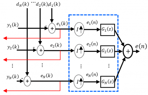
As an additional or optional stage, our attention is directed towards the synthesis filter bank that is placed in the output of the proposed algorithm. In some applications, such as acoustic noise reduction, speech enhancement and acoustic echo cancellation, the full-band output signal is required and must be calculated. For this aim, in our methodology, an interpolation block as illustrated in Figure 4 is integrated. The process of precisely reconstructing the entire error signal across all frequencies involves interpolating the $N$ output error sub-signals and using $G_1(z), \ldots, G_N(z)$.
Figure 4. The detailed bloc for creating full-band signal
The interpolated sub-errors are calculated as follows:
$\begin{cases}e_1(n)= \begin{cases}e_1\left(\frac{k}{I}\right) & n=0, \pm I, \pm 2 I, \ldots \\ 0 & { otherwise }\end{cases} \\ e_2(n)= \begin{cases}e_2\left(\frac{k}{I}\right) & n=0, \pm I, \pm 2 I, \ldots \\ 0 & { otherwise }\end{cases} \\ e_N(n)= \begin{cases}e_N\left(\frac{k}{I}\right) & n=0, \pm I, \pm 2 I, \ldots \\ 0 & { otherwise }\end{cases} \end{cases}$ (54)
The general formula for the N interpolated error sub-signals and full-band output signal is the following:
$e_i(n)=\left\{\begin{array}{cl}e_i\left(\frac{k}{I}\right) & n=0, \pm I, \pm 2 I, \ldots \\ 0 & { otherwise }\end{array}\right.$ (55)
$e(n)=\sum_{i=1}^N \boldsymbol{g}_i^T(n) \boldsymbol{e}_i(n)$ (56)
where, $\mathbf{g}_i(n)=\left[g_i(n), g_i(n-1), \ldots, g_i(n-L+1)\right]^{\mathrm{T}}$, and $\boldsymbol{e}_i(n)=\left[e_i(n), e_i(n-1), \ldots, e_i(n-L+1)\right]^{\mathrm{T}}$.
In this experimental section, a series of experiments were conducted involving a proposed sub-band proportionate separated variable-step-sizes NLMS algorithm within four acoustic impulse response identification, noted respectively, (i) More-Sparse, (ii) Sparse, (iii) Dispersive, and (iv) More Dispersive.
The primary goal is to evaluate the performance of this version while preserving the inherent characteristics of real acoustical rooms. The evaluation was carried out using two types of input signals, both sampled at a frequency of 8 kHz.
The experimental setup is based on four acoustic impulse response, visualized in Figure 5. These impulse responses were employed for all simulations and results presented in this study with different lengths: $M=128,256,512\ and\ 1024$. The sparseness level of impulse response can be computed as follow [27]:
$\zeta=\frac{M}{M-\sqrt{M}} \frac{1-\left\|\boldsymbol{h}_1\right\|}{\sqrt{M}\left\|\boldsymbol{h}_2\right\|}$ (57)
where, $\|.\|_1$ and $\|.\|_2$ denote respectively $l_1$ and $l_2$ norms, and $M$ represent the length of the impulse response. The experiments were conducted over 100,000 iterations.
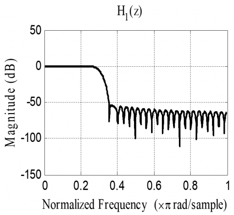
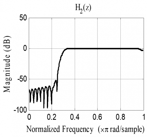
To achieve an effective sub-band decomposition of the signals $x(n)$ and $d(n)$, we used the analysis filters whose length has been deliberately set be proportionate to a parameter $N$. We conducted experiments with $N$ equal to 2 and $L$ equal to 16 . In Figure 6 the frequency representation of the analysis and synthesis filter banks is shown.
These filter banks are designed with a focus on utilizing two sub-bands in the context of employing variable-step-sizes algorithms.
Figure 5. Four types of impulse responses used in simulations
Figure 6. Frequency representation of $H_1(n)$ and $H_2(n)$ with L = 16
4.1 Parameter values and simulation procedure
The assessment of an adaptive algorithm tracking capability is a very important aspect in various applications, particularly those involving dynamic and variable environments. Tracking capability refers to the algorithm's inherent skill to rapidly adapt to changes in input conditions, ensuring consistent and accurate responses. This attribute is particularly crucial in like noise reduction in audio or echo cancellation applications where the input data, such as signals or parameters, show rapid changes and fluctuations. Table 1 shows the used constants and variable parameters. Where they are chosen carefully to ensure firstly, the stability and secondly to find the highest performances of the algorithms by numerous trials.
4.2 Stability study
Assessing the stability of an adaptive algorithm against white noise involves ensuring it can consistently perform well despite random disturbances. In our simulation, white noise represents unpredictable fluctuations that could challenge the algorithm stability. The analysis is centered on how well the adaptive filter maintains convergence and steady-state behavior in the presence of white noise. The evaluation of stability uses the MSE measure. The main objective is to confirm the convergence to best values without showing irregular behavior caused by the white noise.
Table 1. Algorithms parameters
|
Algorithms |
Parameters |
|
NLMS |
$\mu_n=0.9, \varepsilon=10^{-6}, N=1$, |
|
PNLMS |
$\begin{gathered}\mu_n=0.9, \varepsilon=10^{-6}, N=1, \\ \rho=5 / M, \delta=0.01, \mu=0.001\end{gathered}$ |
|
S-NLMS |
$\mu_i=0.9, \varepsilon=10^{-6}, N=2$ |
|
SP-NLMS |
$\begin{gathered}\mu_i=0.9, \varepsilon=10^{-6}, N=2 \\ \rho=5 / M, \delta=0.01, \mu=0.001\end{gathered}$ |
|
MPNLMS |
$\begin{gathered}\mu_n=0.9, \varepsilon=10^{-6}, N=1 \\ \rho=5 / M, \delta=0.01, \mu=0.001\end{gathered}$ |
|
Proposed |
$\begin{gathered}\mu_{max }=0.9, \mu_{min }=0.005, \varepsilon=10^{-6}, N=2, \\ \rho=5 / M, 0<\lambda_i<1,0<\rho_i, \\ \delta=0.01, \mu=0.001\end{gathered}$ |
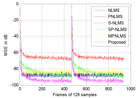
Figure 7. MSE performance using white noise, M = 128
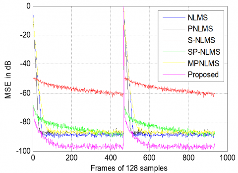
Figure 8. MSE performance using white noise, M = 256
Figures 7 and 8 presents the outcomes achieved using six algorithms: basic NLMS, proportionate NLMS, sub-band NLMS, sub-band proportionate NLMS, $\mu$-law PNLMS (MPNLMS) and proposed SPV-NLMS. In Figure 7, a sparse impulse response with 128 taps was used. The results presented in Figure 8 used a dispersive impulse response with $M=256$.
Based on obtained results presented in Figures 7 and 8, the proposed SPV-NLMS algorithm is a robust candidate, in both types of impulse responses, having an improved convergence and tracking abilities.
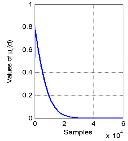
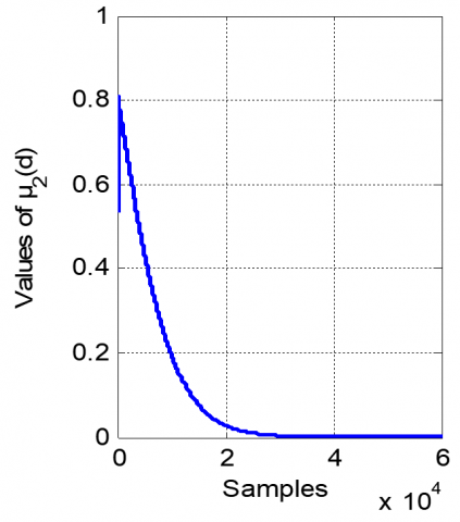
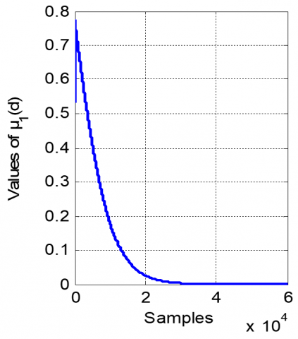
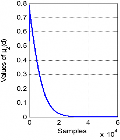
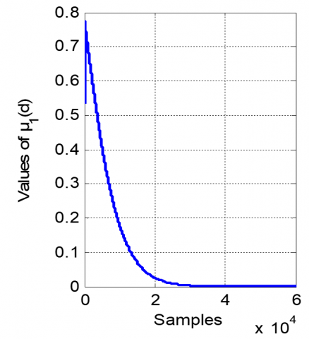
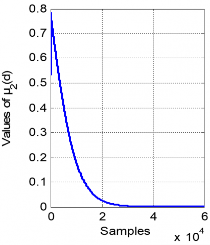
4.3 Time evolution of the proposed separated variables-step-sizes
This simulation part involves the optimization of the proposed sub-band proportionate separated variable-step-sizes NLMS algorithm across consistent parameters and various types of acoustic impulse responses. By applying these refined parameters to different acoustic impulse response systems (More Dispersive, Dispersive, Sparse, and More-Sparse) the study seeks to assess the algorithm adaptability and effectiveness.
Figure 9. Variation of proposed separated step-size parameters in more-dispersive IR case
Figure 10. Variation of proposed separated step-size parameters in dispersive IR case
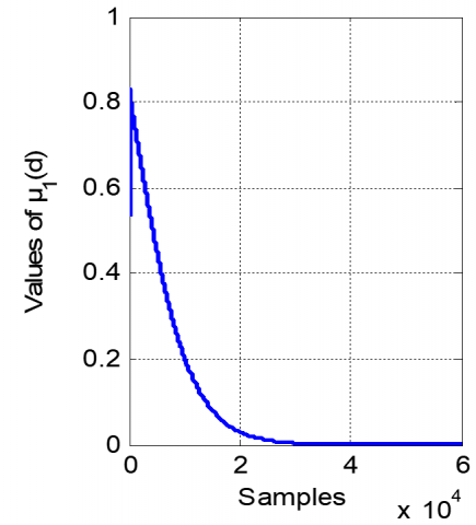
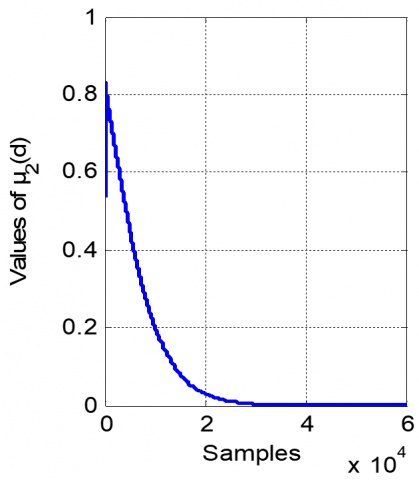
The observed minimization of the separated step-sizes over time, as depicted in Figures 9-12, holds significant implications for the adaptability and convergence behavior of the proposed algorithm. This temporal reduction in step-sizes suggests a proactive response to evolving acoustic conditions. Initially, larger step-sizes are chosen to obtain a rapid convergence during the algorithm early stages, optimizing the estimation process. As the algorithm iterates, the step sizes progressively decrease, indicating a cautious and refined approach to adaptation. This dynamic adjustment allows the algorithm to strike a balance between rapid convergence and low final MSE values. The decreasing step-sizes signify the algorithm ability to fine-tune its learning process, mitigating potential overshooting or divergence issues that might arise in complex and changing acoustic environments. This behavior is particularly relevant in real-world scenarios where maintaining accurate estimates over time is essential. The trend aligns with the algorithm goal to strike a balance between rapid convergence and long-term stability for diverse acoustic scenarios.
Figure 11. Variation of proposed separated step-size parameters in sparse IR case
Figure 12. Variation of proposed separated step-size parameters in more-sparse IR case
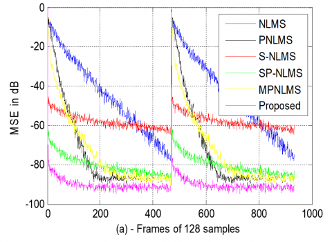
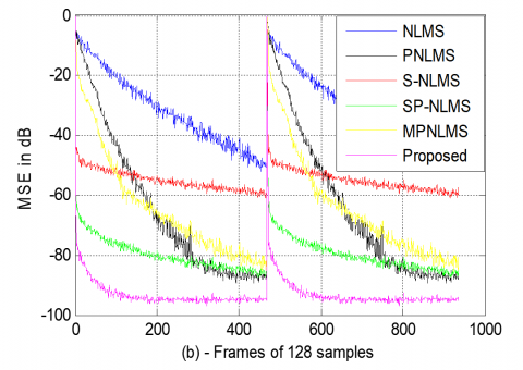
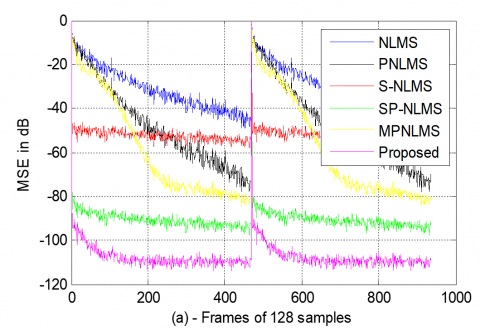
4.4 MSE performance
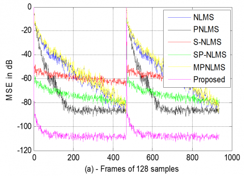
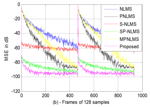
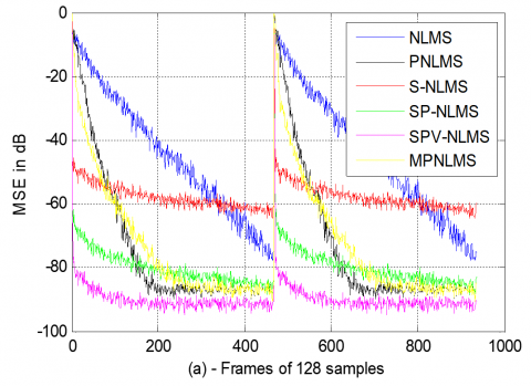
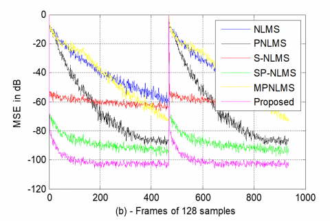
The convergence rate plays an important role in assessing the efficiency and adaptability of different adaptive signal processing algorithms, specifically focusing on the NLMS adaptation. The convergence rate signifies how rapidly an algorithm refines its estimations to reach stable and accurate results during iterative updates. To measure this convergence speed, the MSE criterion is used. The evolution of MSE values is illustrated in Figures 13-16, using the USASI noise under consistent conditions, $\mu=\mu_{max }=0.5$.
We evaluated these algorithms across four distinct noisy acoustic systems with dimensions M = 128 and 256 using four types of acoustic systems, More-Dispersive, Dispersive, Sparse and More-Sparse. This investigation primarily centers on the comparative analysis of six algorithms.
By analyzing the MSE extracted from Figures 13-16, we can readily discern the performance of the first full-band NLMS variant within dispersive IR (Figures 13 and 14). Notably, the conventional FNLMS algorithm also exhibits unsatisfactory performance in scenarios characterized by sparsity (see Figures 15 and 16). However, the proportionate version gives the best performance compared with classical NLMS. The S-NLMS presents a good algorithm in convergence speed but a very modest performance in MSE values in different acoustical systems. After implementing the proportionate strategy on Sub-band NLMS algorithm (SP-NLMS), a fast convergence rate and the same final MSE values compared with other algorithms (S-NLMS, PNLMS, MPNLMS, and the basic NLMS algorithm) are obtained. Also, it can be noticed that the proposed SPV-NLMS algorithm has a very fast convergence; its superiority is proved by the low final MSE values in different acoustical environments compared with S-NLMS, PNLMS, MPNLMS, and the basic NLMS algorithms. This suggests that the proposed algorithm adapts to dynamic changes in acoustic conditions, making it a potential favourite for applications demanding rapid adjustments, such as echo cancellation and noise reduction in communication systems.
Figure 13. MSE evaluation of simulated and proposed algorithms in more-dispersive IR case, with M = 128 in (a) and M = 256 in (b)
Figure 14. MSE evaluation of simulated and proposed algorithms in dispersive IR case, with M = 128 in (a) and M = 256 in (b)
Figure 15. MSE evaluation of simulated and proposed algorithms in sparse IR case, with M = 128 in (a) and M = 256 in (b)
Figure 16. MSE evaluation of all algorithms in more-sparse IR case, with M = 128 in (a) and M = 256 in (b)
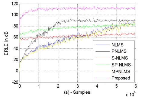
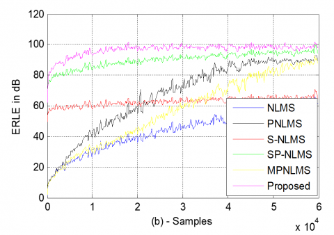
4.5 ERLE performance
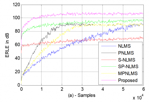
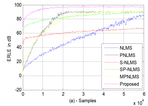
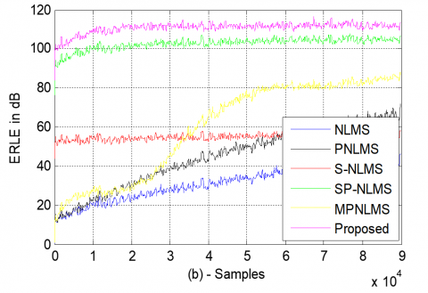
The objective ERLE criterion serves as a good measure for evaluating the efficacy and performance of the proposed SPVNLMS algorithm under conditions similar to those previously announced (see Section 4.4). ERLE, a ratio measure of the residual echo power to the input near-end signal power, offers insight into the algorithm ability to attenuate undesired echoes while preserving the clarity and intelligibility of near-end signal. The ERLE performance is illustrated in Figures 17-20 for acoustic systems employing the USASI noise, $\mu=$ $\mu_{\max }=0.5$.
Figure 17. ERLE evaluation of all algorithms in the more-dispersive IR case, with M = 128 in (a) and M = 256 in (b)
By assessing the ERLE criterion in the same conditions as previously established, the effectiveness of the SPV-NLMS algorithm is proved. Higher ERLE values indicate superior echo suppression and, consequently, a higher level of overall performance in scenarios characterized by acoustic echo, making it a consistent level for validating the proposed algorithm capabilities in mitigating acoustic echoes and enhancing communication quality.
The ERLE results provide a comprehensive view of the algorithmic performance, specifically highlighting the proposed SPV-NLMS algorithm superiority over SP-NLMS, S-NLMS, P-NLMS, MPNLMS and the basic NLMS algorithm.
The proposed algorithm consistently outperforms S-NLMS and P-NLMS due to its innovative combination of sub-band processing and proportionate separated step-sizes. In contrast to the basic NLMS, the proposed algorithm demonstrates significant improvements, underscoring the limitations of uniform step-sizes in handling complex impulse response types. Therefore, the proposed algorithm is well-suited for real applications requiring effective and reliable signal cancellation.
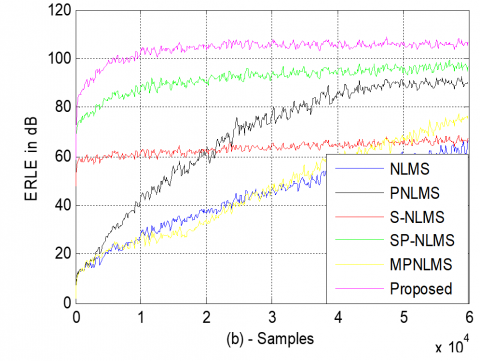
Figure 18. ERLE evaluation of all algorithms in dispersive IR case, with M = 128 in (a) and M = 256 in (b)
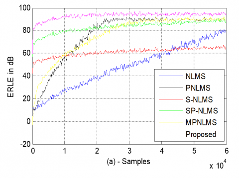
Figure 19. ERLE evaluation of simulated and proposed algorithms in the sparse IR case, with M = 128 in (a) and M = 256 in (b)
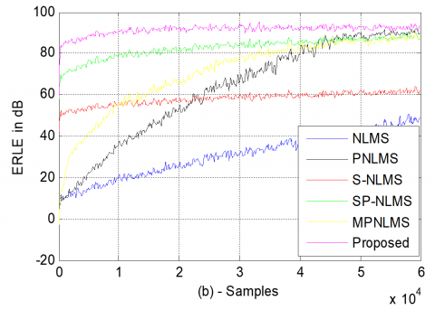
Figure 20. ERLE evaluation of simulated and proposed algorithms in more-sparse IR case, with M = 128 in (a) and M = 256 in (b)
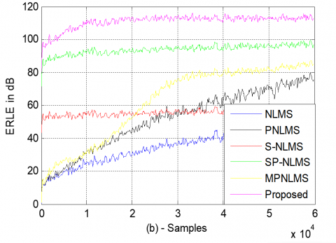
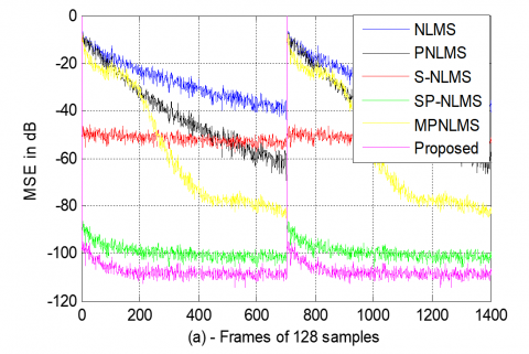
4.6 Proposed algorithm performance in acoustical long impulse response sparse system
Within the experimental framework outlined in this section, a comprehensive experiment was presented to evaluate the proposed algorithm in the context of long impulse responses. These impulse responses, characterized by lengths of M = 512 and 1024, were integrated into the simulation scenarios having sparse systems using two objective criteria, MSE and ERLE, and using the USASI noise with $\mu=\mu_{\max }=0.5$.
Figure 21. Performance of all algorithms in the sparse IR case with M = 512, MSE in (a) and ERLE in (b).
Figure 22. Performance of all algorithms in the sparse IR case with M = 1024, MSE in (a) and ERLE in (b)
In simulation results presented in Figure 21, a sparse impulse response with 512 taps was used. In the next simulation (see Figure 22), the same type of impulse response but with M = 1024 was used.
The detailed analysis of the experimental outcomes, as evaluated by both the MSE and ERLE criteria, proves that the SPV-NLMS algorithm consistently outperforms its counterparts, showcasing its ability to handle and suppress echoes across different acoustic environments
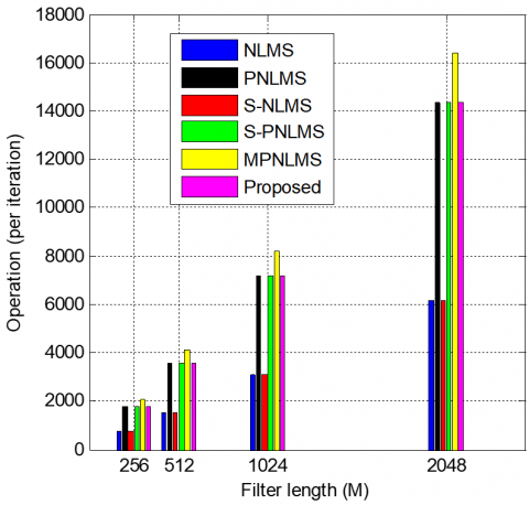
4.7 Numerical complexities
It is necessary to examine the computational complexity of an algorithm. This complexity is relative to mathematical operations in adaptation process. We define the number of operations taken by the algorithm in one iteration. Table 2 below shows computational complexity of classical NLMS, S-NLMS, MPNLMS and the proposed algorithm.
Table 2. Computational complexity
|
Algorithm |
Multiplication |
Division |
Logarithm |
|
NLMS |
3 M + 2 |
1 |
0 |
|
S-NLMS |
3 M + 3 N + 1 |
1 |
0 |
|
PNLMS |
6 M + 3 |
M + 3 |
0 |
|
S-PNLMS |
6 M + 3 N + 4 |
M + 3 |
0 |
|
MPNLMS |
7 M + 3 |
M + 3 |
M |
|
Proposed |
6 M + 3 N + 1 |
M + 5 |
M |
As shown in Table 2, the computational costs for the adaptation process are analyzed in terms of the number of multiplications, divisions, and logarithmic operations required per iteration. Compared to other algorithms such as NLMS, S-NLMS, and MPNLMS, the proposed SPV-NLMS algorithm demonstrates a manageable increase in computational requirements, specifically. The number of multiplications is 6M + 3N + 1, which is comparable to other advanced variants like S-NLMS and lower than MPNLMS. While divisions and logarithmic operations are slightly higher than NLMS and S-NLMS, the cost is significantly optimized compared to MPNLMS.
Figure 23. Computational complexity comparison of simulated algorithms in function of filter length
In addition, Figure 23 presents a representation of the computational complexity, where the slope of the proposed algorithm demonstrates an acceptable level of complexity compared to other simulated algorithms.
To assess real-time applicability and feasibility in resource-constrained environments (e.g., embedded systems), we are conducting simulations and tests on platforms with limited computational power. Preliminary findings suggest that with optimizations such as fixed-point arithmetic and hardware-level parallelism, the algorithm can meet real-time constraints.
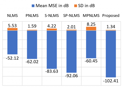
4.8 MSE and standard deviation
The standard deviation analysis of the simulated algorithms, presented in Figures 24 and 25, serves to validate the consistency of the observed performance improvements. We note that the standard deviation is calculated after convergence.
Figure 24. Mean MSE and standard deviation bar chart of simulated algorithms in sparse IR case
Figure 25. Mean MSE and standard deviation bar chart of simulated algorithms in dispersive IR case
This SD analysis provides a statistical measure of variation, confirming the reliability and robustness of the enhancements across different scenarios.
Based on two Figures 24 and 25, the proposed algorithm outperforms all compared methods in both sparse and dispersive impulse response (IR) cases, achieving the lowest Mean MSE (-111.77 dB for sparse IR and -102.41 dB for dispersive IR) and the smallest Standard Deviation (1.58 dB and 1.34 dB, respectively). These results highlight its superior accuracy and consistency, as it effectively minimizes error and variability compared to other algorithms such as NLMS, PNLMS, S-NLMS, SP-NLMS, and MPNLMS, which exhibit higher error levels and greater variability. This demonstrates the robustness and adaptability of the proposed method in diverse acoustic scenarios.
This research paper provides a detailed investigation into the performance and effectiveness of the proposed SPV-NLMS algorithm for identifying various acoustic impulse responses. The algorithm is designed based on a sub-band structure, with each sub-filter utilizing individual proportionate step sizes. The study begins by establishing the novelty of the proposed algorithm in comparison to existing classical NLMS variants. A comprehensive derivation of the variable step size is presented, followed by an in-depth mathematical analysis of the algorithm's stability.
Through extensive simulations and analyses, the SPV-NLMS algorithm demonstrates robust performance, superior stability, a fast convergence rate, and remarkably low MSE values across diverse acoustic scenarios, including More-Dispersive, Dispersive, Sparse, and More-Sparse environments. The research examines various aspects of the algorithm, including stability under white noise conditions using MSE criteria. Notably, the proposed algorithm consistently outperforms other NLMS variants, highlighting its adaptability, accuracy, and efficiency. It effectively manages challenges introduced by USASI noise, maintains stable convergence, and achieves low final MSE values. By integrating sub-band processing with separate variable step-size adjustments, the algorithm excels in handling complex and dynamic acoustic systems, making it an ideal solution for applications requiring high stability, precise convergence, and dependable results.
Furthermore, the algorithm’s strong ERLE performance in suppressing residual signals underscores its effectiveness in echo cancellation tasks, proving its suitability for practical applications. As a potential future direction, the implementation of the proposed algorithm on digital signal processors and its application in real-world acoustic echo cancellation scenarios is recommended.
|
LMS |
Least Means Square |
|
NLMS |
Normalized Least Means Square |
|
SPV-NLMS |
Sub-band Proportionate Variable-step-size NLMS |
|
MSE |
Means Square Error |
|
ERLE |
Echo Return Loss Enhancement |
|
MSD |
Means Square Diviation |
|
USASI |
USA Standards Institute. |
|
IR |
Impulse Response |
|
FNLMS |
Fast NLMS |
|
P-NLMS |
Proportionate NLMS |
|
S-PNLMS |
Sub-band NLMS |
|
MPNLMS |
µ_law Proportionate NLMS |
|
Greek symbols |
|
|
$\alpha(n)$ |
Normalized Factor |
|
$\mu_n$ |
Fixed Step-Size |
|
$\alpha_i(k)$ |
normalization factors link to ith input sub-signals |
|
$\mu_i(k)$ |
Individual variable step-size parameters assigned to ith sub-filters |
|
$\delta, 0, \lambda$ |
Regularization components |
|
$\mu, \xi$ |
Positive Quantities |
|
$\boldsymbol{\epsilon}_i(k)$ |
weight-error vector |
|
$\Delta_i(k)$ |
Small Quantity |
|
$\mu_{max }$ |
Maximal Step-Size value |
|
$\mu_{min }$ |
Minimal Step-Size value |
|
$\varepsilon$ |
Small Positive Constant |
|
Subscripts |
|
|
M |
Lenth of Impulse Response |
|
L |
Length of sub-filter |
|
D |
Down-sampling factor |
|
N |
Number of the Sub-band |
[1] Haykin, S., Widrow, B. (2003). Least Mean Square Adaptive Filters. Wiley. https://doi.org/10.1002/0471461288
[2] Rashmi, R., Jagtap, S. (2019). Adaptive noise cancellation using NLMS algorithm. Soft Computing and Signal Processing. Advances in Intelligent Systems and Computing, 898: 515-525, https://doi.org/10.1007/978-981-13-3393-4_53
[3] Ciochină, S., Paleologu, C., Benesty, J. (2016). An optimized NLMS algorithm for system identification. Signal Processing, 118: 115-121. https://doi.org/10.1016/j.sigpro.2015.06.016
[4] Dakulagi, V., Dakulagi, R., Yeap, K.H., Nisar, H. (2023). Improved VSS-NLMS adaptive beamformer using modified antenna array. Wireless Personal Communications, 128(4): 2741-2752. https://doi.org/10.1007/s11277-022-10068-7
[5] Li, J., Stoica, P. (2006). Robust Adaptive Beamforming. Hoboken, NJ: John Wiley.
[6] Benesty, J., Paleologu, C., Ciochină, S., Kuhn, E.V., Bakri, K.J., Seara, R. (2022). LMS and NLMS algorithms for the identification of impulse responses with intrinsic symmetric or antisymmetric properties. In ICASSP 2022-2022 IEEE International Conference on Acoustics, Speech and Signal Processing (ICASSP), Singapore, Singapore, pp. 5662-5666. https://doi.org/10.1109/ICASSP43922.2022.9747430
[7] Kim, H.W., Kim, H.J., Choi, J.Y. (2020). Multiparameter identification for SPMSMs using NLMS adaptive filters and extended sliding‐mode observer. IET Electric Power Applications, 14(4): 533-543. https://doi.org/10.1049/iet-epa.2019.0643
[8] Prasad, S.R., Patil, S.A. (2016). Implementation of LMS algorithm for system identification. In 2016 International Conference on Signal and Information Processing (IConSIP), Nanded, India, pp. 1-5. https://doi.org/10.1109/ICONSIP.2016.7857460
[9] Janjanam, L., Saha, S.K., Kar, R., Mandal, D. (2021). An efficient identification approach for highly complex non-linear systems using the evolutionary computing method based Kalman filter. AEU-International Journal of Electronics and Communications, 138: 153890. https://doi.org/10.1016/j.aeue.2021.153890
[10] Bellanger, M. (2024). Adaptive filtering. In Digital Signal Processing (Chap 14). https://doi.org/10.1002/9781394182695.ch14
[11] Bendoumia, R. (2021). New sub-band proportionate forward adaptive algorithm for noise reduction in acoustical dispersive-and-sparse environments. Applied Acoustics, 175: 107822. https://doi.org/10.1016/j.apacoust.2020.107822
[12] Duttweiler, D.L. (2000). Proportionate normalized least-mean-squares adaptation in echo cancelers. IEEE Transactions on Speech and Audio Processing, 8(5): 508-518. https://doi.org/10.1109/89.861368
[13] Benesty, J., Gay, S.L. (2002). An improved PNLMS algorithm. In 2002 IEEE International Conference on Acoustics, Speech, and Signal Processing, Orlando, USA, pp. II-1881-II-1884. https://doi.org/10.1109/ICASSP.2002.5744994
[14] Deng, H., Doroslovacki, M. (2005). Improving convergence of the PNLMS algorithm for sparse impulse response identification. IEEE Signal Processing Letters, 12(3): 181-184. https://doi.org/10.1109/LSP.2004.842262
[15] Das, P., Deb, A., Kar, A., Chandra, M. (2014). A unique low complexity parameter independent adaptive design for echo reduction. In Advanced Computing, Networking and Informatics- Volume 1, 27: 33-40. https://doi.org/10.1007/978-3-319-07353-8_5
[16] Husøy, J.H. (2022). A simplified normalized subband adaptive filter (NSAF) with NLMS-like complexity. In 2022 International Conference on Applied Electronics (AE), Pilsen, Czech Republic, pp. 1-5. https://doi.org/10.1109/AE54730.2022.9919894
[17] Abadi, M.S.E., Kadkhodazadeh, S. (2011). A family of proportionate normalized subband adaptive filter algorithms. Journal of the Franklin Institute, 348(2): 212-238. https://doi.org/10.1016/j.jfranklin.2010.11.003
[18] Abadi, M.S.E. (2009). Proportionate normalized subband adaptive filter algorithms for sparse system identification. Signal Processing, 89(7): 1467-1474. https://doi.org/10.1016/j.sigpro.2008.12.025
[19] Yu, Y., Ye, J., Zakharov, Y., He, H. (2023). Robust proportionate subband adaptive filter algorithms with optimal variable step-size. IEEE Transactions on Circuits and Systems II: Express Briefs, 71(4): 2444-2448. https://doi.org/10.1109/TCSII.2023.3328779
[20] Bekrani, M., Khong, A.W. (2020). A delayless sub-band PNLMS adaptive filter for sparse channel identification. In 2020 28th Iranian Conference on Electrical Engineering (ICEE), Tabriz, Iran, pp. 1-6. https://doi.org/10.1109/ICEE50131.2020.9260596
[21] Yu, Y., Zhao, H. (2016). A band-independent variable step size proportionate normalized subband adaptive filter algorithm. AEU-International Journal of Electronics and Communications, 70(9): 1179-1186. https://doi.org/10.1016/j.aeue.2016.05.016
[22] Liu, J.M. (2016). Adaptive filters for sparse system identification. Doctoral Dissertations, Missouri University of Science and Technology. https://www.proquest.com/openview/46cba630d5f89ae394669a408554f4f0/1?pq-origsite=gscholar&cbl=18750.
[23] Roman, N., Wang, D. (2005). A pitch-based model for separation of reverberant speech. In Proceedings of Interspeech, Lisbon.
[24] Iannelli, A., Yin, M., Smith, R.S. (2021). Experiment design for impulse response identification with signal matrix models. IFAC-PapersOnLine, 54(7): 625-630. https://doi.org/10.1016/j.ifacol.2021.08.430
[25] Ribas, C.H., Bermudez, J.C., Bershad, N.J. (2012). Identification of sparse impulse responses–design and implementation using the partial Haar block wavelet transform. Digital Signal Processing, 22(6): 1073-1084. https://doi.org/10.1016/j.dsp.2012.06.004
[26] Becker, A.C., Kuhn, E.V., Matsuo, M.V., Benesty, J. (2024). On the NP-VSS-NLMS algorithm: Model, design guidelines, and numerical results. Circuits Syst Signal Process 43: 2409-2427. https://doi.org/10.1007/s00034-023-02565-2
[27] Albu, F., Kwan, H.K. (2013). New proportionate affine projection sign algorithms. In 2013 IEEE International Symposium on Circuits and Systems (ISCAS), Beijing, China, pp. 521-524. https://doi.org/10.1109/ISCAS.2013.6571895