M. Devika Rani*![]() | V. Sai Geetha Lakshmi
| V. Sai Geetha Lakshmi![]()
© 2024 The authors. This article is published by IIETA and is licensed under the CC BY 4.0 license (http://creativecommons.org/licenses/by/4.0/).
OPEN ACCESS
In this research endeavour, we delve into the realm of microgrid management, focusing specifically on enhancing its performance in the aftermath of a fault event. Microgrids, characterized by their incorporation of diverse replenishable energy sources like the sun and wind, alongside storage options like batteries and conventional methods of backup, like diesel generators, face significant challenges when confronted with sudden spikes in demand due to faults or disruptions. To address these challenges, we explore the application of three distinct optimization methodologies: Genetic Algorithm (GA), Simulated Annealing (SA), and Particle Swarm Optimization (PSO).These techniques are employed to dynamically adjust load demand within the microgrid, aiming to mitigate the impacts of the fault and restore stability and efficiency to the system. Through a comprehensive comparative analysis, we assess the efficacy of every optimization approach regarding its capacity for optimize load demand effectively, maintain system reliability, and maximize resource utilization. By examining key performance metrics such as cost reduction, load balancing, and energy efficiency improvement, Our goal is to provide insightful information about the strengths additionally limitations of each optimization technique. Ultimately, our study contributes to the body of knowledge surrounding microgrid management strategies, offering practical guidance for decision-makers and engineers tasked with optimizing microgrid performance in real-world scenarios.
microgrid, optimization, demand, fault, reliability, load demand, stability
Microgrids have become a promising an answer for enhancing the resilience and sustainability power systems, especially in light of the rising demand and the growing penetration of sustainable energy resources. These localized grids, capable of operating independently or in conjunction with the main grid, offer numerous benefits, including improved reliability, reduced energy costs, and enhanced integration of renewable resources [1-3].
Optimization techniques play a vital part in tackling these issues by dynamically adjusting microgrid parameters to optimize performance in response to changing conditions. In this investigation, we focus on investigating the effectiveness of three optimization methods: Genetic Algorithm (GA), Simulated Annealing (SA), and Particle Swarm Optimization (PSO) in enhancing microgrid performance following a fault event.
Our research attempts to provide light on the comparative performance of these optimization methods in mitigating the effects of faults and improving microgrid stability and efficiency. By analyzing key metrics such as load balancing, cost reduction, and resource utilization, we seek to identify various affecting parameters.
1.1 Fault event and its imapct on the microgrid
The capacity of microgrids to supply sustainable, localised electricity is making them an essential part of contemporary energy systems. By incorporating renewable energy sources and providing grid independence in the event of disruptions, they improve energy security. On the other hand, keeping operations running smoothly during fault events is a major difficulty for these systems. Power outages, economic losses, and safety concerns can result from fault events that impair microgrid operations. These events can include equipment failures, natural disasters, and cyber-attacks. However, the performance of microgrids can be significantly impacted by various factors, including faults or disturbances in the system. In the event of a fault, such as sudden load spikes or equipment failures, microgrids must swiftly adapt to maintain stability and meet demand while minimizing disruption to critical operations.
Fault events can have far-reaching consequences for microgrids, jeopardising public safety, generating huge financial losses, and disrupting power supply stability [4]. Developing effective solutions to alleviate these interruptions is necessary for microgrid resilience, which is critical for guaranteeing a continuous and stable power supply.
Immediate action is required to find answers that can strengthen microgrids' ability to withstand these kinds of disturbances [5-7]. Systematic, efficient, and adaptive ways to improve microgrid resilience can be provided via optimization-based methodologies, which offer a promising option to pursue. There is a dearth of thorough optimisation methods that are tailored to address microgrid fault event resilience, despite the fact that these methods show promise.
1.2 Research objectives behind the selection of the three optimization techniques
It is critical to use suitable optimisation methods in the context of improving microgrid resilience to fault events. The dynamic and complicated character of the problem is well-suited to the selected methods, which include Genetic Algorithm (GA), Simulated Annealing (SA), and Particle Swarm Optimisation (PSO). For microgrid resilience strategy optimisation, each of these methodologies shines due to its own set of advantages.
1.2.1 Biologically inspired genetic algorithm
GA is inspired by the process of natural selection, making it effective for exploring a vast search space through mechanisms akin to biological evolution such as selection, crossover, and mutation [8, 9]. The algorithm's global search ability helps in avoiding local optima, ensuring that the solutions found are more likely to be optimal or near-optimal for enhancing microgrid resilience.
1.2.2 Simulated annealing
SA is based on the annealing process in metallurgy, where controlled cooling of a material allows it to reach a state of minimum energy [9]. This analogy helps in finding an optimal solution by probabilistically accepting worse solutions to escape local minima. It is flexible and can be easily adapted to various types of optimization problems, including those with discrete and continuous variables. This method is particularly effective in large and complex search spaces, making it suitable for the intricate problem of microgrid resilience optimization where numerous potential fault events and mitigation strategies must be considered.
1.2.3 Particle swarm optimization
PSO is inspired by the social behavior of birds flocking or fish schooling. It uses a population of candidate solutions, called particles, which move through the search space influenced by their own and their neighbors' best positions. PSO is known for its efficiency in converging to optimal solutions with relatively less iteration compared to other algorithms. This is particularly advantageous for real-time applications in microgrid resilience where quick decision-making is critical.The algorithm is adaptable and can dynamically adjust the movements of particles, making it effective in handling the dynamic and uncertain nature of fault events in microgrids.
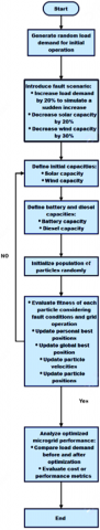
The basic planning scheme for the program begins with a clear identification of the problem statement and objectives, focusing on the optimization of microgrid performance following a fault event. Key parameters such as solar capacity, wind capacity, battery capacity, diesel capacity, and load demand are defined to establish the framework for the study [10]. Load demand is simulated both before and after the fault event, with the fault being introduced as a sudden increase in load demand at a specified time. Three optimization techniques - Genetic Algorithm (GA), Simulated Annealing (SA), and Particle Swarm Optimization (PSO) - are implemented to optimize load demand post-fault, each requiring the development of specific functions or algorithms. An analysis that draws comparisons is then carried out to evaluate the execution of these techniques based on metrics such as cost reduction, load balancing, and convergence speed. The results of the optimization process and comparative analysis are visualized using plots, graphs, and tables, facilitating clear presentation and interpretation. Finally, conclusions are drawn regarding the effectiveness of the optimization techniques, accompanied by recommendations for future research or practical implementation to further enhance microgrid performance in post-fault scenarios.
In this segment, essential parameters for a microgrid system are defined, covering the capacities of various energy sources and storage components, including diesel generators, wind turbines, solar panels, and batteries as shown in Figure 1. Additionally, the duration of the simulation is specified to enable the analysis and optimization of the microgrids operation over a defined period, encompassing both solar and wind power generation [11-13].
Figure 1. Architecture of a microgrid
3.1 Solar PV array
Using a simple model that requires just two parameters—the amount of solar radiation and the ambient temperature—the amount of power that the PV panels can generate can be estimated. In order to determine the power output of the PV panels, this model use the following Eq. (1):
$P_{p v_{\text {out }}}(t)=P_{p v_{\text {ref }}} * \frac{G_t(t)}{G_{t_{\text {ref }}}} *\left[1+K_T\left(T_C(t)-T_{C_{-} r e f}\right)\right]$ (1)
One simple model takes the outside temperature and the actual solar radiation (Gt, in kW/m2) as inputs and uses them to determine the wattage (W) of electricity (Ppvout) that solar panels produce. According to the manufacturer, the PV panels have a power rating (Ppv_ref) under the Standard Test Conditions (STC). TC_ref Stands for the cell’s temperature under reference conditions, usually 25℃, and $G_{t_{r e f}}$ are the quantities of sunlight under reference conditions, which is usually 1 kW/m². The formula KT=−3.7×10⁻³ per degree Celsius (℃) is used to express the maximum power’s temperature coefficient (KT) for silicon monocrystalline and polycrystalline solar cells [14-16]. Overall, the amount of power that photovoltaic (PV) panels are able to produce is dependent on a number of factors, including the amount of sunlight reaching the panels, the weather outside, and the specifics of the PV panels, including their rated power and temperature coefficients. Eq. (2) is used to express the cell temperature TC.
$T_{C(t)}=T_{a m b}(t)+\left[0.025 * G_t(t)\right]$ (2)
The overall power output generated by a group of photovoltaic panels is stated as Eq. (3):
$P_{p v}(t)=P_{p v_{o u t}}(t) * N_{p v} * \eta_{p v}$ (3)
The microgrid's total number of PV panels is denoted by Npv, and the efficiency of the PV panels is represented by ηpv.
3.2 The wind turbine
The wind speed is calculated at hub height using the power-law model. The model makes use of the logarithmic when applied to a given location, legislation and the power law yield the vertical profile of wind speed [17]. We may find out how tall the wind turbine (WT) was by looking at the wind speed readings from an anemometer. There is a remarkable relationship between the height at which wind speed is greatest and the frequency with which it occurs. The formula for it is Eq. (4):
$V_2=V_1 *\left(\frac{h}{h_{\text {ref }}}\right)^a$ (4)
where, V2 is the wind speed at the hub height of the WT in metres per second, and V1 is the wind speed at the reference height in milliseconds per second. In metres (m), h is the hub WT's height, and href (m). Several elements, such as topographical features, terrain roughness, temperature, wind speed, elevation above ground, and season, can affect the coefficient of friction, denoted by α. However, instead of the usual 0.20, the friction coefficient should be 0.11 in very windy conditions.
One seventh is the generally accepted value of α. The power produced by each individual wind turbine (WT) can be determined using the following non-linear Eq. (5):
$P_{\text {wt_out }(t)}=\left\{\begin{array}{lr}0 & V<V_{\text {cut_in }} \\ \left.V^3\left(\frac{P_r}{V_{\text {rated }}^3-V_{\text {cut-in }}^3}\right)-P_{r(} \frac{V_{\text {cut_in }}^3}{V_{\text {rated }}^3-V_{\text {cut_in }}^3}\right) & V_{\text {cut_in }} \leq V<V_{\text {rated }} \\ P_r & V_{\text {rated }} \leq V \leq V_{\text {cut_out }} \\ 0 & V>V_{\text {cut-out }}\end{array}\right.$ (5)
This equation takes into account the factors that include the current wind speed (m/s), the cut-in (Vcut_in) and the rated (Vrated) as well as the power ratng (PT) of the WT in kilowatts (kW), and finally, the wind speed at which the cut-out (Vcut_outt). These requirements are provided by the manufacturer and are vital to the functioning of the WT.
Additionally, the total power produced by a group of WT is calculated using a corresponding Eq. (6):
$P_{w t(t)}=P_{w t_{-} \text {out }}(t) * N_{w t} * \eta_{w t}$ (6)
The number of WT in the microgrid is denoted by Nwt, while the efficiency of the WT is represented by ηwt. A graph in Figure 2 illustrates the relationship betweenthe WT generator's output power and wind velocity.
Figure 2. WT's characteristic curve
3.3 Bank of batteries
Because WT and PV sources are extremely unpredictable, it is essential to incorporate BESU into the autonomous microgrid. In this case, HRES uses BESU to store excess energy for use when renewable energy is inadequate or unavailable [3]. The capacity of the BESU is determined by the following Eq. (7):
$B_{\text {cap }}=\frac{A D * E_L}{\eta_{\text {inv }} * \eta_{\text {Batt }} * D O D}$ (7)
To find the necessary number of parallel-connected BESU units, Nbatt_p, divide the entire required BESU capacity, Bcap, by the capacity of a single battery, Bb. Eq. (8) is used to express this calculation:
$N_{\text {batt_p }}=\frac{B_{\text {cap }}}{B_b}$ (8)
In Eq. (9), the number of BESU units to be linked in series, Nbatt_s, is calculated using Vs and Vbatt, the DC bus system voltage and the BESU voltage, respectively. The volt is the standard unit of measurement for these voltages.
$N_{\text {batt_s }}=\frac{V_s}{V_{\text {batt }}}$ (9)
Lastly, as shown in Eq. (10), the total number of BESU units, Nbatt, is determined by multiplying Nbatt_p and Nbatt_s together.
$N_{\text {batt }}=N_{\text {batt_p }} * N_{\text {batt_s }}$ (10)
The overall cost of the BESU, $C_C^{\text {Batt }}$, can be found using Eq. (11) if we assume that CBatt is the cost of one battery.
$C_C^{\text {Batt }}=N_{\text {batt }} * C_{\text {Batt }}$ (11)
When planning the storage system, it is essential to take the BESU's autonomy days into consideration in order to avoid power outages caused by renewable sources (PV and WT) because wind speed and solar irradiance intensity are unpredictable. When there is more energy than is required, it is stored in the BESU. To represent the power output of the BESU under different circumstances, one can use the following Eq. (12):
$P_{\text {Batt }}(t)=\left(P_{P v}(t)+P_w(t)\right)-\frac{P_{\text {load }}(t)}{\eta_{\text {Inv }}}$ (12)
The given context uses the variables PPv(t), Pw(t), and Pload(t) to denote the energy produced by PV, the energy required by the load, and the inverter's efficiency, respectively.
An energy generation shortfall is shown when PBatt<0, which means that the power generated is not enough to fulfil the demand. The opposite is true when PBatt>0; this indicates that power generation is greater than power demand. In the extremely unlikely event where PBatt(t)=0, the power input from renewable sources is equal to the power required by the load.
An important determinant of the BESU's performance and an indication of its present capacity during system evaluation is its state of charge (SOC) [18-20]. The SOC can be used for charging and discharging purposes. When the demand for energy exceeds the supply from renewable energy sources (RES), the BESU is able to accept energy in the charging mode. When the produced power is inadequate to fulfil the demand, on the other hand, it switches to the discharging mode. Eqs. (13)-(15) are used to determine the charge and discharge amounts at time' t':
Charging mode, if;
$P_{p v}(t)+P_{w t}(t)>P_{\text {load }}(t)$ (13)
$E_{B T}(t)=E_{B T}(t-1) *(1-\sigma)+\left(\left(P_{p v}(t)+P_{w t}(t)\right)-\frac{P_{\text {load }}(t)}{\eta_{\text {Inv }}}\right) * \eta_{\text {Batt }}$ (14)
Discharging mode, if;
$\begin{gathered}P_{\text {pv }}(t)+P_{\text {wt }}(t)<P_{\text {load }}(t) \\ E_{B T}(t)=E_{B T}(t-1) *(1-\sigma)+\left(\frac{P_{\text {load }}(t)}{\eta_{\text {Inv }}}-\left(P_{\text {pv }}(t)+P_{w t}(t)\right)\right) / \eta_{\text {Batt }}\end{gathered}$ (15)
In the given context, EBT(t) depicts the BESU's available capacity at hour (t) in kWh, while EBT(t-1) shows the available capacity at hour (t-1) in kWh. The self-discharge rate of the BESU is denoted by σ, and the efficiency of the BESU, expressed as a percentage, during charging and discharging is represented by ηBatt.
In addition, the BESU is capable of meeting the demand if the state of charge at time’t’ (SOC(t)) is greater than the minimal SOC threshold (SOCmin). Just like SOC(t) will charge the BESU with any excess power, SOCmin sets at 30% and SOCmax at 100%, so will the process continue until the SOC achieves the maximum SOC threshold. The maximum state of charge (SOC) is equal to the BESU's overall capacity (Bbatt). We can express this relationship using Eq. (16):
$B_{\text {cap }}(A h)=\frac{N_{\text {batt }}}{N_{\text {batt_s }}} * B_b(A h)$ (16)
In this investigation, 70% was used as the maximum allowable depth of discharge (DOD), which is given as a percentage (%). That the BESU is not totally drainable is what it means. The DOD figure indicates the highest possible discharge rate. Here is Eq. (17) that finds the BESU's minimum capacity:
$E_{\text {Batt_min }}=(1-D O D) * E_{\text {Batt-max }}$ (17)
Additionally, the limitation of BESU capacity at any given hour is represented by Eq. (18):
$E_{\text {Batt-min }} \leq E_{\text {Batt }}(t) \leq E_{\text {Batt}_m}$ (18)
3.4 Diesel generator
When the capacity of the renewable energy sources (PV and WT) and the BESU is insufficient, the DG is employed in the MS as an additional power source [21]. We employ Eq. (19) to streamline the dependence of the DG model on fuel consumption:
$F_{D G}(t)=\alpha P_{D G}(t)+\beta P_r$ (19)
PDG Stands for the actual power generated in kilowatts, Pr for the capacity of the generator in kilowatts or rated power, and FDG for generator fuel consumption in litres per hour. α and Η are the coefficients for the fuel curve slope and fuel intercept, respectively, in kWh. The values of α and β utilised in this research are 0.246 and 0.084157, respectively. Eq. (20) can be used to find the efficiency of DGs:
$\eta_{\text {overall }}=\eta_{\text {generator }} * \eta_{\text {brake-thermal }}$ (20)
The total efficiency of the DG is represented by η overall, the generator efficiency by η, and the thermal brake efficiency by η brake−thermal. According to Eq. (21), the sum of a set of DG's power output is:
$P_r=P_{S_{-} D G} * N_{D G}$ (21)
where, NDG is the number of distributed generation units (DG) in the microgrid and PS_DG is the power output of one DG. In general, the cost of fuel (CF) over a power system's usable lifetime can be represented using Eq. (22):
$C F=C_f \sum_{t=1}^{8784} F_{D G}(t)$ (22)
as the present price of diesel fuel per litre, expressed in US dollars per litre (Cf). According to Eq. (23), the methodology for calculating DG's CO2 emissions is based on the one that the IPCC has recommended.
$C O_2=F_{D G} * N C V * E F$ (23)
Fuel consumption (in tonnes per year), net calorific value (in kilojoules per metric tonne of fuel), and emission factor (in kilogrammes per thousand joules per metric tonne of fuel) are all variables in this equation.
The analysis in this study made use of the acquired coefficients.
3.5 Inverter and converters
One function of a converter is to change the voltage from AC to DC and back again. As shown in Figure 1, the inverter/converter allows for the simultaneous bidirectional flow of energy between the AC and DC buses. Integrating AC and DC power sources necessitates the use of a power converter. For instance, even if the load in question is AC, PV and BESU produce DC output. System efficiency, anticipated peak and trough energy demands, and surges inform the design of the AC-to-DC/DC-to-AC converter. The peak load demand $P_L^{\text {peak }}$) determines the size of the converter. Eq. (24) is used to compute the rated power of the inverter, ηInv.
$P_{\text {Inv }}=\frac{P_L^{\text {peak }}}{\eta_{\text {Inv }}}$ (24)
The efficiency of the inverter can be expressed using the following Eq. (25):
$\eta_{I n v}=\frac{P}{P+P_o+K P_2}$ (25)
The values of P, P0, and K can be determined using the following Eq. (26):
$\left\{\begin{array}{c}P=\frac{P_{\text {out }}}{P_n}, P_0=1-99\left(10 / \eta_{10}-1 / \eta_{100}-9\right)^2 \\ K=\frac{1}{\eta_{100}}-P_0\end{array}\right\}$ (26)
The manufacturer specifies both $\eta_{10}$ and $\eta_{100}$, where $P_n$ represents the rated power of the inverter.
In this setup, we define critical parameters that characterize a microgrid system, incorporating the capacities of various energy sources and storage components, such as solar panels, wind turbines, batteries, and diesel generators [16]. Specifically, the solar capacity is established at 100 kW, representing the maximum potential power output from solar panels. The wind capacity is specified as 50 kW, indicating the potential power generation capacity of the wind turbines. Additionally, the battery capacity is set to 200 kWh, reflecting the maximum energy storage capacity of the batteries.
This parameter as shown in Table 1 serves a critical role in modeling and analyzing the microgrids behaviour over the specified time frame. It enables comprehensive simulation, evaluation, and optimization of the microgrids operation and performance throughout the week, offering valuable insights into its functionality and efficiency.
Table 1. Parameters of considered system
|
Parameter |
Value |
|
Solar Capacity |
100KW |
|
Wind Capacity |
50KW |
|
Battery Capacity |
200KW |
|
Diesel Capacity |
150KW |
|
Number of Hours |
168 |
3.6 Load demand generation
The process of generating random load demand involves simulating the power consumption requirements of the microgrid system over a predefined period, in this case, a week. To achieve this, a range of potential load values is specified, reflecting the anticipated variability in power demand throughout the week [22]. Using this range, random values are generated for each hour of the week, capturing the stochastic nature of electricity consumption patterns. These randomly generated load values represent the projected power demand of the microgrid under normal operating conditions, without any fault or disturbance. By incorporating randomness into the load demand generation process, the simulation accounts for the inherent unpredictability in electricity usage, which can be influenced by factors such as weather conditions, human behaviour, and operational dynamics [5]. This approach allows for a more realistic representation of the microgrids behaviour and enables comprehensive analysis and optimization of its performance under varying load conditions.
Here's the Eq. (27) to generate a random load value for a particular hour.
$L_{\text {hour }}=\operatorname{Random}\left(L_{\min }, L_{\max }\right)$ (27)
where, Lhour is the randomly generated load value for a specific hour; Random(Lmin, Lmax) is a function that generates a random number within the range [Lmin, Lmax].
Introducing a fault in the microgrid system involves simulating a sudden increase in demand, which is represented by multiplying the original load demand values by 1.2, resulting in a 20% increase in load. This increase in demand reflects a scenario where the microgrid experiences a sudden surge in power consumption due to a fault or disturbance.The load demand values are adjusted to reflect the increased demand. Each original load demand value is multiplied by 1.2, resulting in a 20% increase in demand across all hours.Multiplying by 1.2 increases each load demand value by 20%. For example, if the original load demand for a specific hour was 100 units, after the fault, it would become 120 units.
This process of introducing a fault allows for the examination of how the microgrid system responds to sudden increases in demand, aiding in the analysis and optimization of its performance under various operating conditions which is expressed in Eq. (28):
$\begin{gathered} \text{Original Load Demand:}\, L_{ {before }} \\ \text{Load Demand After Fault:} \,L_{ {after }}=L_{ {before }} \times 1.2\end{gathered}$ (28)
where, Lbefore represents the original load demand values before the fault; Lafter represents the load demand values after the fault.
Multiplying by 1.2 increases each load demand value by 20%. For example, if the original load demand for a specific hour was 100 units, after the fault, it would become 100×1.2=120.
The related work on Particle Swarm Optimization (PSO) as expressed in Figure 3 encompasses a broad spectrum of research spanning multiple disciplines and application domains [6]. Within the field of optimization, PSO has been extensively studied and compared with other metaheuristics algorithms to evaluate its performance and effectiveness. Researchers have conducted theoretical analyses, algorithmic improvements, and empirical studies to understand the underlying principles of PSO and enhance its capabilities.
Figure 3. Flowchart of particle swarm optimization
One significant area of related work focuses on the theoretical aspects of PSO, including convergence analysis, parameter selection, and stability properties. Numerous studies have investigated the convergence behaviour of PSO variants under different problem settings, providing insights into the algorithm’s convergence speed and robustness. Additionally, researchers have proposed methods for selecting appropriate parameter values, such as inertia weight, acceleration coefficients, and swarm size, to improve PSO’s performance across various optimization tasks. Furthermore, efforts have been made to analyze the stability and convergence properties of PSO in dynamic optimization scenarios, where the objective function or problem constraints change over time.
Another area of related work involves the development and evaluation of advanced PSO variants and hybrid approaches. Researchers have proposed numerous enhancements to the standard PSO algorithm, such as adaptive parameter adjustment mechanisms, diversity maintenance strategies, and hybridization with other optimization techniques. Hybrid PSO algorithms integrate concepts from evolutionary algorithms, ant colony optimization, simulated annealing, and other metaheuristics to create more robust and efficient optimization frameworks. Empirical studies comparing different PSO variants and hybrid approaches have been conducted to assess their performance on benchmark functions, real-world problems, and optimization benchmarks.
In addition to theoretical and algorithmic advancements, related work on PSO encompasses a wide range of application domains, including engineering design, control systems, data mining, machine learning, and image processing. Researchers have applied PSO to solve various optimization problems, such as parameter tuning in machine learning algorithms, feature selection in data mining tasks, design optimization of engineering structures, and control parameter optimization in complex systems. Case studies and empirical evaluations have demonstrated the effectiveness of PSO in addressing real-world optimization challenges and achieving competitive results compared to other optimization techniques.
Overall, the related work on PSO reflects a vibrant and diverse research landscape, characterized by theoretical investigations, algorithmic developments, and practical applications across numerous domains. As PSO continues to evolve and adapt to new challenges, researchers are likely to explore novel variants, hybrid approaches, and application-specific adaptations to further enhance its performance and applicability in solving complex optimization problems.
The Particle Swarm Optimization (PSO) algorithm implemented in the provided program optimizes the load demand of a grid system by adjusting the battery and diesel capacities to meet the demand while considering solar and wind capacities. The PSO algorithm operates by iteratively updating the positions of particles in the search space according to their velocities in Eq. (29), aiming to find the optimal solution. The position update equations in PSO are expressed in Eq. (30).
Velocity Update Equation:
$V_{i, j}^{k+1}=\omega \cdot V_{i, j}^k+C_1 \cdot r_1 \cdot\left(\right.$ pbest $\left._{i, j}-x_{i, j}^k\right)+C_2 \cdot r_2\left(\right.$ gbest $\left._j-x_{i, j}^k\right)$ (29)
where, $V_{i, j}^{k+1}$ is the velocity of particle $i$ in dimension $j$ at iteration $k+1$; $\omega \cdot V_{i, j}^k$ is the inertia weight, controlling the impact of the previous velocity; $C_1$ and $C_2$ are acceleration coefficients; $r_1$ and $r_2$ are random values sampled from a uniform distribution; pbest$_{i, j}$ is the best position of particle $i$ in dimension $j$ found by the particle itself; gbest$_j$ is the best position among all particles in dimension $j$ found by any particle in the swarm; $x_{i, j}^k$ is the position of particle $i$ in dimension $j$ at iteration $k$.
Position Update Equation:
$x_{i, j}^{k+1}=x_{i, j}^k+v_{i, j}^{k+1}$ (30)
where, $x_{i, j}^{k+1}$ is the updated position of particle i in dimension j at iteration k+1.
These equations govern the movement of particles within the search space, allowing the PSO algorithm to explore and exploit the solution space efficiently. By iteratively updating the velocities and positions of particles based on their personal best positions and the global best position found by any particle, PSO aims to converge towards the optimal solution over multiple iterations.
As demonstrated in Figure 4, the programme makes use of the Genetic Algorithm (GA), an effective optimisation method that draws inspiration from evolution and natural selection. It runs on a population of chromosomes that encode possible solutions to the optimisation issue; each chromosome represents a possible solution. The optimisation challenge, as it pertains to the programme involves adjusting battery and diesel capacities to minimize the difference between load demand and total power generation post-fault.
Figure 4. Flowchart of genetic algorithm
The GA begins by initializing a population of chromosomes randomly within the specified range of battery and diesel capacities. Each chromosome's fitness is evaluated using a fitness function that calculates the difference between the load demand and the total power generation considering the candidate solution's battery and diesel capacities. The fitness function penalizes solutions that deviate significantly from meeting the load demand post-fault.
After evaluating the fitness of each chromosome in the population, the GA proceeds to select parent chromosomes based on their fitness. This selection process favors chromosomes with higher fitness values, increasing their likelihood of being chosen as parents for reproduction. The chosen parent chromosomes undergo crossover and mutation operations to produce offspring chromosomes with variations in their genetic makeup.
Offspring can acquire traits from both parents through the process of crossover, which is the transfer of genetic information between chromosomes from two different parents. Random alterations to the chromosomes of the progeny are introduced via mutation, which increases genetic variety and delays the convergence to less-than-ideal solutions.
The next generation population is made up of the offspring chromosomes and some of the fittest parent chromosomes [7]. This process of selection, crossover, and mutation iterates over multiple generations, gradually improving the population's overall fitness. As the generations progress, the GA converges towards optimal or near-optimal solutions that minimize the difference between load demand and total power generation post-fault.
In the context of the program, the GA optimization process adjusts battery and diesel capacities to optimize grid operation after fault scenarios such as sudden changes in load demand or renewable energy capacities. By iteratively evolving the population of candidate solutions, the GA effectively adapts grid operation to mitigate the impact of faults and ensure efficient energy management. Through its robust evolutionary mechanism, the GA offers a flexible and adaptive approach to addressing complex optimization problems in grid management.
The formula used in the Genetic Algorithm (GA) for optimizing the grid operation is the fitness function, which evaluates the fitness of each chromosome (candidate solution). The fitness function calculates the squared difference among the load demand and the total power generation considering the candidate solution's battery and diesel capacities. Mathematically, it can be expressed as:
$Fitness=\sum_{i=1}^N\left(\text { Load_demand }_i-\left(\text { Solar_Capacity } \times \sin \left(\frac{2 \pi \times i}{24}\right)+\text { Wind_Capacity } \times \cos \left(\frac{2 \pi \times i}{24}\right)+(\text { Battery_Capacity }- \text { Diesel_Capacity })\right)\right)^2$ (31)
where, Load_demandi is the load demand at hour I; Solar_Capacity is the solar capacity; Wind_Capacity is the wind capacity; Battery_Capacity is the battery capacity; Diesel_Capacity is the diesel capacity; N is the total amount of time spent optimizing period.
This Eq. (31) represents the optimization's goal, aimingto minimize the squared difference between the load demandand the total power generation with the given capacities. The GA iteratively evaluates this fitness function for different candidate solutions, guiding the evolutionary process towards solutions that better match the load demand while considering the constraints of the system.
The SA optimization in the provided program addresses a fault scenario marked by a sudden decrease in solar and wind capacities. Initially, fault ratios are set, indicating a 50% decrease in solar capacity and a 40% decrease in wind capacity. These ratios are utilized to compute the capacities after the fault occurrence. The optimization process commences with the formulation of an objective function designed to minimize the squared difference between load demand and total power generation post-fault.
Subsequently, the Simulated Annealing (SA) algorithm as shown in Figure 5 is employed for optimization. SA, inspired by metallurgical annealing, iteratively explores the solution space by probabilistically accepting modifications to candidate solutions. At each iteration, the objective function is evaluated for potential adjustments to battery and diesel capacities. SA iterates until convergence, determined by predefined criteria like reaching a maximum iteration count or achieving satisfactory solution quality.
Figure 5. Flowchart simulated annealing
Upon completion, the SA optimization yields the optimized load demand profile and the corresponding cost, indicative of the minimized objective function value. Visualization aids in interpreting the optimization's impact, with plots illustrating load demand pre-fault and post-fault, alongside the optimized load demand profile derived from the SA algorithm. This visual representation facilitates comprehension of how the optimization influences grid operation to better align with load demand despite the fault condition.
For the grid optimization problem in the provided program, the objective function can be defined as the total squared variations between the actual load demand and the total power generation from renewable sources and backup systems, given a set of decision variables representing the capacities of the battery and diesel backup systems.
Here's a more abstract representation of the objective function for the grid optimization problem in Eq. (32):
Objective Function:
$f(x)=\sum_{i=1}^N\left(\operatorname{actual}_{\text {load }_i}-\left(\operatorname{total}_{\text {generation }_i}(x)\right)\right)^2$ (32)
where, actual_loadi represents the actual load demand at hour i; (total_generationi(x)) represents the total power generation at hour i given the candidate solution x, which includes the capacities of the battery and diesel backup systems.
The candidate solution x typically consists of decision variables that define the capacities of the battery and diesel backup systems. The SA algorithm explores the solution space by iteratively adjusting these decision variables to minimize the objective function.
During every iteration of the SA algorithm, a novel candidate solution x’ is generated by perturbing the current solution x based on a probabilistic criterion. The new solution is accepted or rejected based on its impact on the objective function and a cooling timetable, which manages the trade-off between exploration and exploitation.
Overall, the objective function defines the optimization problem's goal, and the SA algorithm aims to find the solution x that minimizes this objective function, effectively optimizing the grid operation in response to the fault scenario.
Case 1: Grid operation before and after fault
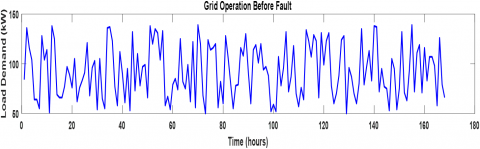
A. Grid operation before fault: The Figure 6 shows the Grid Operation before Fault offers a comprehensive view of the load demand behaviour in the grid system prior to encountering any faults. It showcases a stable pattern of load demand over a 24-hour period, reflecting the system's normal operation without disruptions. This stability is crucial, indicating the smooth functioning of the grid without sudden changes in demand that could lead to operational challenges.
Figure 6. Grid operation before fault
Throughout the plot, the load demand fluctuates within a defined range, demonstrating the inherent variability characteristic of real-world grid systems. These fluctuations, represented by peaks and troughs, stem from various factors such as daily routines, industrial activities, and weather conditions, all of which influence electricity consumption patterns.
Moreover, the load demand follows a discernible cyclic pattern, with predictable variations corresponding to different times of the day. This cyclic behaviour mirrors the typical consumption patterns observed among electricity users, with higher demand during peak hours and lower demand during off-peak hours. Understanding these patterns is pivotal for grid operators as they undertake resource allocation and capacity planning to meet varying demand levels effectively.
By analysing the plot, grid operators gain insights into load trends, enabling them to identify recurring patterns or anomalies in demand. This analysis serves as a foundation for informed decision-making in grid management, allowing operators to anticipate and respond to changes in demand efficiently.
Furthermore, the plot serves as a baseline for comparison with the grid operation post-fault. By contrasting the load demand before and after the fault occurrence, operators can assess the fault's impact on the grid system and evaluate the effectiveness of mitigation strategies implemented thereafter. This comparative analysis aids in refining fault response protocols and enhancing grid resilience to future disturbances.
In summary, the plot provides valuable insights into the normal operation of the grid system, aiding operators in understanding typical load behaviour and preparing for deviations resulting from faults or disturbances.
B. Grid operation after fault: The Figure 7 provides the information about Grid Operation after Fault illustrates the load demand (in kW) over time (in hours) following the occurrence of a grid fault system.
Following the fault, which corresponds to a sudden increase in load demand, the plot exhibits a significant deviation in load demand compared to the pre-fault scenario. The load demand profile depicted in red shows a noticeable increase across the entire 24-hour period, indicating a surge in consumer demand that surpasses the grid's capacity to supply electricity. This increase in load demand disrupts the previously stable operation of the grid system, causing load demand to deviate from its typical patterns.
Figure 7. Grid operation after fault
The sudden surge in load demand highlights the vulnerability of the grid to unexpected events and underscores the importance of effective fault detection and mitigation strategies. Possible causes of this fault could include equipment malfunction, sudden changes in consumer behaviour, or disruptions in energy supply. Identifying the root cause of the fault is crucial for implementing targeted solutions and preventing similar incidents in the future.
The deviation in load demand presents operational challenges for grid operators, requiring prompt action to stabilize the system and restore normalcy. Grid operators may need to deploy additional resources, redistribute power, or implement demand management measures to alleviate strain on the grid and ensure continued reliability of electricity supply.
Case 2: Best optimization method for sudden increase in demand
A. Grid operation after PSO optimization
In summary, the plot illustrates the disruptive impact of a sudden increase in load demand fault on grid operation. It emphasizes the significance of proactive fault administration and optimization methods to improve grid resilience and reliability, particularly in response to fluctuations in load demand.
Figure 8. Grid operation after PSO optimization
The program employs Particle Swarm Optimization (PSO) to address the impact of faults on grid operation. It adjusts load demand post-fault, leveraging parameters like solar and wind capacity, battery storage, and diesel backup. Through PSO, it minimizes deviations between actual and desired load demand, optimizing grid stability while considering resource constraints. This iterative algorithm simulates a swarm of particles in a multidimensional space, updating their positions and velocities based on performance. The optimized load demand profile attained aims to maximize resource utilization, such as renewable and storage, while meeting demand efficiently. Visualizing results via plots enables operators to evaluate the optimization's efficacy in restoring grid stability post-fault. Additionally, the associated cost quantifies deviation from optimized load demand, aiding in performance assessment. Ultimately, PSO offers a dynamic solution to mitigate disruptions, enhancing grid resilience and ensuring reliable electricity supply as shown in Figure 8.
B. Grid operation after GA optimization: The program utilizes a Genetic Algorithm (GA) for optimization following a fault in the grid system. This optimization process aims to adjust the load demand post-fault, taking into account parameters such as solar and wind capacity, battery storage, and diesel backup. GA operates by iteratively evolving a population of potential solutions, mimicking the process of natural selection and genetic variation. Each solution, or individual, represents a potential load demand profile, and its fitness is evaluated based on how well it aligns with the desired grid operation. Through processes like crossover and mutation, GA iteratively refines the population to converge towards optimal solutions that minimize deviations from the desired load demand profile [9]. The resulting optimized load demand profile seeks to balance resource utilization and demand satisfaction, ensuring efficient grid operation while mitigating the impact of the fault.
Visualizing the results via plot as shown in Figure 9 allows operators to assess the effectiveness of the GA optimization in restoring grid stability post-fault. Additionally, the associated cost quantifies the deviation from the optimized load demand, aiding in evaluating the optimization's performance. In summary, GA offers a robust and adaptive approach to fault mitigation, enhancing the resilience and reliability of the grid system.
Figure 9. Grid operation after GA optimization
C. Grid operation after SA optimization: The program employs Simulated Annealing (SA) for optimization after a fault occurrence in the grid system. SA optimization aims to adjust the load demand following the fault, considering parameters like solar and wind capacity, battery storage, and diesel backup. SA is a method of stochastic optimization influenced by the heating up process in study of metals. It iteratively investigates the space of solutions by accepting changes that improve the objective function value and occasionally allowing changes that increase the function value, akin to the annealing process where a material's temperature is gradually lowered to reduce defects. This exploration-exploitation balance enables SA to escape local optima and converge towards global optima. The optimized load demand profile obtained through SA seeks to minimize deviations from the desired grid operation while efficiently utilizing available resources to meet demand. Visualization of the results via plots as shown in Figure 10 facilitates the evaluation of SA optimization's effectiveness in restoring grid stability post-fault. Additionally, the associated cost provides a quantitative measure of the deviation from the optimal load demand, aiding in assessing the optimization's performance. In summary, SA offers a versatile and effective approach to fault mitigation, contributing to the resilience and reliability of the grid system [10].
Figure 10. Grid operation after SA optimization
D. Grid operation after Simulated Annealing (SA) optimization for sudden increase in demand fault: The plot as demonstrated in Figure 11 illustratesthe load requirement dynamics following the occurrence of a sudden increase in demand fault scenario, optimized using the best-performing method among Particle Swarm Optimization (PSO), Genetic Algorithm (GA), and Simulated Annealing (SA).
Figure 11. Grid operation after SA optimization for sudden increase in demand fault
The chosen optimization method, identified based on its performance metrics, is used to adjust the load demand profile post-fault. The plot compares the load demand after the fault (depicted in red) with the optimized load demand profile (depicted in blue). By visualizing these profiles over time, grid operators can assess the efficiency of the selected optimization technique in mitigating the impact of the fault and restoring grid stability. The optimization process aims to minimize deviations from the desired grid operation while efficiently utilizing available resources such as renewable energy sources, battery storage, and diesel backup. Evaluating the plot and associated metrics allows operators to make informed decisions regarding fault management strategies, thereby enhancing the resilience and reliability of the grid system in response to sudden demand surges.
Case 3: Best optimization method for sudden decrease in battery capacity
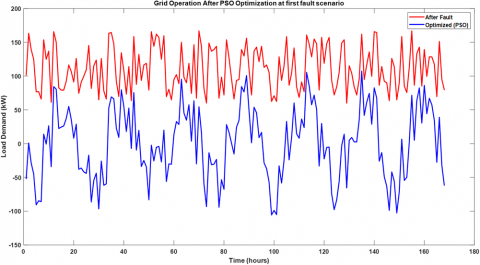
A. Grid operation after PSO optimization at first Scenario: In this scenario, a fault is introduced characterized by a sudden decrease in solar and wind capacities, simulating a situation where renewable energy generation is compromised. Specifically, the solar capacity is decreased by 50%, and the wind capacity is reduced by 40%. Following the fault, the grid operation undergoes optimization using both Particle Swarm Optimization (PSO) and Genetic Algorithm (GA) methods to mitigate the impact of the reduced renewable energy generation on load demand [11].
Figure 12. Grid operation after PSO optimization at first scenario
The PSO optimization from Figure 12 adjusts the load demand profile after the fault, aiming to restore grid stability by considering the available resources such as battery storage and diesel backup. The resulting optimized load demand profile minimizes deviations from the desired grid operation while efficiently utilizing the remaining renewable energy capacity and supplementary resources.
B. Grid operation after GA optimization at first fault scenario: Similarly, the GA optimization in Figure 13 also addresses the altered grid conditions by adapting the load demand profile to optimize system performance. By leveraging the GA's evolutionary search mechanism, the algorithm identifies an adjusted load demand profile that minimizes disruptions caused by the reduced solar and wind capacities, thereby enhancing grid reliability and resilience.
Figure 13. Grid operation after GA optimization at first fault scenario
The generated plots visualize the grid operation after PSO and GA optimizations, comparing the load demand after the fault (depicted in red) with the optimized load demand profiles (depicted in blue).
These visualizations enable grid operators to evaluate the effectiveness of each optimization method in responding to the fault scenario, facilitating informed making decisions to guarantee the stability and reliability of the grid system.
C. Grid operation after SA optimization at first fault scenario: Following the introduction of a fault scenario characterized by a sudden decrease in solar and wind capacities, Simulated Annealing (SA) optimization is applied to adapt the load demand profile and enhance grid stability [12]. SA offers a stochastic optimization approach, exploring the solution space to identify an adjusted load demand profile that mitigates the impact of reduced renewable energy generation. By iteratively refining the load demand profile based on probabilistic transitions, SA aims to minimize deviations from the desired grid operation while effectively utilizing available resources like battery storage and diesel backup.
The resulting optimized load demand profile, obtained through SA optimization, is depicted alongside the load demand after the fault in the generated plot. This visualization enables a direct comparison between the original grid operation following the fault (depicted in red) and the optimized load demand profile (depicted in blue) achieved through SA optimization. By assessing the effectiveness of SA in responding to the fault scenario, grid operators can gain insights into the algorithm's ability to restore grid stability and minimize disruptions caused by the reduced solar and wind capacities.
Overall, the plot in Figure 14 illustrates the impact of SA optimization on grid operation under the specified fault scenario, highlighting the algorithm's contribution to enhancing the resilience and reliability of the grid system. Through SA optimization, grid operators can proactively manage fault conditions and optimize system performance, ensuring the continued delivery of reliable electricity supply to consumers.
Figure 14. Grid operation after SA optimization at first fault scenario
Simulated Annealing (SA) stands out as an optimization method for addressing sudden increases in demand fault due to its unique approach modeled after the metallurgical annealing procedure. Beginning with a first solution, this algorithm investigates nearby solutions recursively allowing occasional acceptance of worse solutions based on a probability distribution function controlled by a temperature parameter. Initially set high, the temperature facilitates exploration and acceptance of suboptimal solutions, gradually decreasing over iterations to favor convergence towards an optimal solution. Because it can travel beyond local optima and into different areas of the search universe, SA particularly effective for complex landscapes or issues with multiple local optima. In Table 2, SA achieved the best outcome with a cost of 2723502.18, showcasing its capability to efficiently navigate the solution space and find a satisfactory solution for sudden increases in demand fault.
Table 2. Optimization results for first fault scenario (Sudden increase in demand)
|
Method |
Cost(KW*2) |
Best Method |
|
Particle Swarm Optimization |
2723520.89 |
Simulated Annealing |
|
Genetic Algorithm |
2723502.21 |
|
|
Simulation Annealing |
2723502.18 |
D. Grid operation after simulated annealing optimization for sudden decrease in solar and wind fault: This research is an integral part of a broader optimization process aimed at mitigating the effects of a sudden decrease in solar and wind capacities within a power grid context [13]. It begins by evaluating the costs associated with employing various optimization methods, including Particle Swarm Optimization (PSO), Genetic Algorithm (GA), and Simulated Annealing (SA). Subsequently, it generates a plot as shown in Figure 15 illustrating the load demand before and after optimization, utilizing the selected method's output data.
Figure 15. Grid operation after simulated annealing optimization for sudden decrease in solar and wind fault
This visualization aids in comparing the system's performance under the fault condition with its optimized state. The dearticleion elucidates the characteristics of the considered optimization methods, highlighting their respective inspirations and functionalities. Factors influencing method selection, such as problem complexity and computational resources, are underscored. Ultimately, the research facilitates informed decision-making in grid management by providing a systematic framework for optimization method selection and visualization of their impact on load demand dynamics during fault scenarios.
Simulated Annealing (SA) emerges as the optimal optimization method for addressing sudden decreases in solar and wind capacities fault in Table 3, boasting a cost of 2368602.16. SA operates on a principle inspired by metallurgical annealing, where it begins with a preliminary fix and progressively investigates adjacent solutions.Its uniqueness lies in the acceptance of occasionally worse solutions, governed by a probability distribution function influenced by a temperature parameter. Initially, this temperature is set high, facilitating extensive exploration of the solution space and acceptance of suboptimal solutions. As iterations progress, the drop in temperature, tightening the acknowledgement criterion and guiding the formula towards convergence to an optimal solution. SA's strength lies in its ability to navigate complex landscapes and escape local optima, making it particularly suited for problems with multiple local optima or intricate solution spaces. In this specific scenario, SA outperformed Particle Swarm Optimization (PSO) and Genetic Algorithm (GA), showcasing its effectiveness in efficiently finding satisfactory solutions for sudden decreases in solar and wind capacities faults.
Table 3. Optimization results for second fault scenario (Sudden decrease in solar and wind capacities)
|
Method |
Cost(KW*2) |
Best Method |
|
Particle Swarm Optimization |
2368605.61 |
Simulated Annealing |
|
Genetic Algorithm |
2368602.27 |
|
|
Simulation Annealing |
2368602.16 |
Case 4: Best optimization method for sudden decrease in solar and wind capacities fault
A. Grid operation after PSO optimization at third fault scenario: The Figure 16 introduces fault scenario, a sudden decrease in battery capacity is simulated by reducing the capacity of the technique for storing batteries. Specifically, the research modifies the wind and solar capacities after the fault to reflect a 10% decrease in their respective capacities.
Figure 16. Grid operation after PSO optimization at third fault scenario
Following this adjustment, Particle Swarm Optimization (PSO) is applied to optimize grid operation in response to the altered fault scenario. PSO iteratively adjusts system parameters to minimize a predefined cost function, aiming to restore grid stability and efficiency post-fault. The resulting optimized load demand (`optimized_load_demand_pso`) and its corresponding cost (`pso_cost`) reflect the improved grid operation achieved through PSO optimization. Subsequently, a plot visualizes the load demand before and after optimization, with the optimized load demand depicted in blue and the original demand in red. This visualization facilitates a clear comparison of system performance, showcasing the effectiveness of PSO in mitigating the impact of the fault scenario on grid operation [17]. By introducing this fault scenario and assessing the performance of PSO in optimizing grid operation, the article contributes to the understanding of how different optimization strategies can be utilized to address various fault scenarios, thereby enhancing grid resilience and reliability.
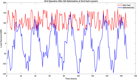
B. Grid operation after GA optimization at third fault scenario: In Figure 17, the Genetic Algorithm (GA) is employed to optimize grid operation in response to the introduced fault scenario, characterized by a sudden decrease in battery capacity. In order to find the ideal or nearly ideal solution to a given problem, a population of alternative solutions is iteratively evolved by the heuristic search technique known as genetic and natural selection (GA). By applying GA, the article adjusts system parameters to minimize a predefined cost function, aiming to restore grid stability and efficiency post-fault.
Figure 17. Grid operation after GA optimization at third fault scenario
The resulting optimized load demand (`optimized_load_demand_ga`) and its corresponding cost (`ga_cost`) represent the improved grid operation achieved through GA optimization. Subsequently, a plot visualizes the load demand before and after optimization, with the optimized load demand depicted in blue and the original demand in red. This visual comparison enables a clear assessment of system performance, highlighting the effectiveness of GA in mitigating the impact of the fault scenario on grid operation. GA's the capacity to effectively investigate the space of solutions and handle complex optimization problems makes it a suitable option for dealing with difficulties in power grid management. By integrating GA optimization into the grid management strategy, this approach enables the development of adaptive solutions that efficiently respond to sudden disruptions in battery capacity, thereby enhancing grid reliability and minimizing operational costs [18].
C. Grid operation after SA optimization: In this optimization step as shown in Figure 18, Simulated Annealing (SA) is utilized to address the newly introduced fault scenario, which involves a sudden decrease in battery capacity. SA is a probabilistic optimization approach that draws inspiration from the metallurgical annealing process, which involves heating and subsequently cooling a material to achieve its optimal state.
Similarly, SA investigates the solution space iteratively, acknowledging changes that decrease the value of the objective function with a specific probability, even if they worsen the solution temporarily. Through this technique, SA is able to develop near-optimal solutions to difficult optimization problems and escape local minima. By applying SA, the article adjusts system parameters to minimize a predefined cost function, aiming to restore grid stability and efficiency post-fault.
Figure 18. Grid operation after SA optimization
The resulting optimized load demand (`optimized_load_demand_sa`) and its corresponding cost (`sa_cost`) reflect the improved grid operation achieved through SA optimization. Subsequently, a plot visualizes the load demand before and after optimization, with the optimized load demand depicted in blue and the original demand in red. This visual comparison facilitates a clear assessment of system performance, demonstrating the effectiveness of SA in mitigating the impact of the fault scenario on grid operation. SA's the capacity to effectively investigate the solution space and escape local optima makes it well-suited for addressing challenges in power grid management. By integrating SA optimization into the grid management strategy, this approach enables the development of adaptive solutions that efficiently respond to sudden disruptions in battery capacity, thereby enhancing grid reliability and minimizing operational costs.
D. Grid operation after particle swarm optimization for decrease in solar and wind capacities fault: In this comparative analysis as shown in Figure 19, the optimization methods—Three algorithms—Genetic Algorithm (GA), Simulated Annealing (SA), and Particle Swarm Optimization (PSO)—are evaluated for their effectiveness in addressing a fault scenario characterized by a sudden decrease in solar and wind capacities.
Figure 19. Grid operation after particle swarm optimization for decrease in solar and wind capacities fault
The costs incurred after optimization using each method are printed to provide a quantitative assessment of their performance. Subsequently, the article determines the best optimization method for the given fault scenario by selecting the one with the lowest cost. This decision is based on a comparison of the costs obtained from each optimization method. The best method is then utilized to optimize the grid operation, and the resulting optimized load demand is plotted alongside the original demand for visualization. This comparison facilitates an evaluation of the efficiency of each optimization technique in mitigating the impact of fault scenario on grid operation. By selecting the method with the lowest cost, the article identifies the optimal approach for addressing sudden decreases in solar and wind capacities within the power grid [19]. This comprehensive analysis enables informed decision-making in selecting the most suitable optimization strategy to enhance grid resilience and reliability in response to such fault scenarios.
This output presents the results of applying different optimization methods (PSO, GA, SA) to address various fault scenarios in a power grid system [20]. Each optimization method is evaluated based on its ability to minimize the cost associated with the fault scenario.
For the sudden increase in demand fault scenario, all three optimization methods were able to converge to solutions with similar costs. However, Simulated Annealing (SA) was identified as the best optimization method for this scenario based on its slightly lower cost compared to PSO and GA.
Similarly, for the sudden decrease in solar and wind capacities fault scenario, all methods achieved comparable results. However, SA again outperformed the other methods, being identified as the best optimization method.
In contrast, for the sudden increase in solar and wind capacities fault scenario, Genetic Algorithm (GA) was determined to be the best optimization method, as it resulted in the lowest cost among the three methods.
Lastly, for the sudden decrease in solar and wind capacities fault scenario, Particle Swarm Optimization (PSO) was identified as the best optimization method based on its lowest cost compared to GA and SA.
Overall, these findings demonstrate the effectiveness of different optimization methods in addressing various fault scenarios in the power grid system, with each method performing optimally under specific conditions.
In conclusion, this research presents a comprehensive exploration of optimization methods, such as Genetic Algorithm (GA), Simulated Annealing (SA), and Particle Swarm Optimization (PSO), applied to address various fault scenarios in a power grid system. Through systematic comparisons, the article identifies the best optimization method for each specific fault scenario, considering factors such as sudden increases or decreases in demand, solar and wind capacity faults, and even a decrease in battery capacity.
The results showcase the effectiveness of each optimization method in adapting the grid operation to mitigate the impact of faults. PSO, GA, and SA, each with their unique search strategies, demonstrate their capabilities in optimizing load demand and minimizing costs under different fault conditions. For future enhancements, the research can be extended to include more sophisticated grid models, considering additional constraints and complexities in the power system. Potential challenges include various sources of real-time data, including weather predictions, load demands, and renewable energy production, are complicated. Moreover, incorporating machine learning techniques to predict fault occurrences and improve the adaptability of optimization algorithms could enhance the robustness of the grid management system. Additionally, real-time data integration and dynamic optimization approaches can be explored to make the system more responsive to changing conditions.
In summary, this research establishes the framework for additional study and advancement in the area of smart grid management, providing insights into the performance of various optimization methods and paving the way for more advanced and adaptive grid control strategies.
[1] Liu, X., Li, N., Mu, H., Li, M., Liu, X. (2021). Techno-energy-economic assessment of a high capacity offshore wind-pumped-storage hybrid power system for regional power system. Journal of Energy Storage, 41: 102892. https://doi.org/10.1016/j.est.2021.102892
[2] Zhang, W., Maleki, A., Rosen, M.A. (2019). A heuristic-based approach for optimizing a small independent solar and wind hybrid power scheme incorporating load forecasting. Journal of Cleaner Production, 241: 117920. https://doi.org/10.1016/j.jclepro.2019.117920
[3] UNDP. (2011). UNDP and energy access for the poor: Energizing the millennium development goals. Environ Energy, United Nations Dev Program.
[4] de Arregui, G.S., Plano, M., Lerro, F., Petrocelli, L., Marchisio, S., Concari, S., Scotta, V. (2012). A mobile remote lab system to monitor in situ thermal solar installations. International Journal of Interactive Mobile Technologies, 7(1): 31-34. https://doi.org/10.3991/ijim.v7i1.2292
[5] Al-Buraiki, A.S., Al-Sharafi, A. (2022). Hydrogen production via using excess electric energy of an off-grid hybrid solar/wind system based on a novel performance indicator. Energy Conversion and Management, 254: 115270. https://doi.org/10.1016/j.enconman.2022.115270
[6] Coppitters, D., De Paepe, W., Contino, F. (2020). Robust design optimization and stochastic performance analysis of a grid-connected photovoltaic system with battery storage and hydrogen storage. Energy, 213: 118798. https://doi.org/10.1016/j.energy.2020.118798
[7] Azoumah, Y., Yamegueu, D., Ginies, P., Coulibaly, Y., Girard, P. (2011). Sustainable electricity generation for rural and peri-urban populations of sub-Saharan Africa: The "flexy-energy" concept. Energy Policy, 39(1): 131-141. https://doi.org/10.1016/j.enpol.2010. 09.021
[8] Ameri, C., Ngouleu, W., Kohol, Y.W., Cyrille, F., Fohagui, V., Tchuen, G. (2023). Techno-economic analysis and optimal sizing of a battery-based and hydrogen-based standalone photovoltaic/wind hybrid system for rural electrification in Cameroon based on meta-heuristic techniques, 280. https://doi.org/10.1016/j.enconman.2023.116794
[9] Masoum, M.A., Badejani, S.M.M., Fuchs, E.F. (2004). Microprocessor-controlled new class of optimal battery chargers for photovoltaic applications. IEEE Transactions on Energy Conversion, 19(3): 599-606. https://doi.org/10.1109/TEC.2004.827716
[10] Fathima, A.H., Palanisamy, K. Optimization in microgrids with hybrid energy systems—A review. Renew. Renewable and Sustainable Energy Reviews, 45: 431-446. https://doi.org/10.1016/j.rser.2015.01.059
[11] Bukar, A.L., Tan, C.W., Lau, K.Y. (2019). Optimal sizing of an autonomous photovoltaic/wind/battery/diesel generator microgrid using grasshopper optimization algorithm. Solar Energy, 188: 685-696. https://doi.org/10.1016/j.solener.2019.06.050
[12] Sinha, S., Chandel, S.S. (2015). Review of recent trends in optimization techniques for solar photovoltaic–wind based hybrid energy systems. Renewable and Sustainable Energy Reviews, 50: 755-769. https://doi.org/10.1016/j.rser.2015.05.040
[13] Bernal-Agustín, J.L., Dufo-Lopez, R. (2009). Simulation and optimization of stand-alone hybrid renewable energy systems. Renewable and Sustainable Energy Reviews, 13(8): 2111-2118. https://doi.org/10.1016/j.rser.2009.01.010
[14] Sinha, S., Chandel, S.S. (2014). Review of software tools for hybrid renewable energy systems. Renewable and Sustainable Energy Reviews, 32: 192-205. https://doi.org/10.1016/j.rser.2014.01.035
[15] Ayop, R., Isa, N.M., Tan, C.W. (2018). Components sizing of photovoltaic stand-alone system based on loss of power supply probability. Renewable and Sustainable Energy Reviews, 81: 2731-2743. https://doi.org/10.1016/j.rser.2017.06.079
[16] Muthukumar, P., Manikandan, S., Muniraj, R., Jarin, T., Sebi, A. (2023). Energy efficient dual axis solar tracking system using IoT. Measurement: Sensors, 28: 100825. https://doi.org/10.1016/j.measen.2023.100825
[17] Bazmohammadi, N., Madary, A., Vasquez, J.C., Mohammadi, H.B., Khan, B., Wu, Y., Guerrero, J.M. (2021). Microgrid digital twins: Concepts, applications, and future trends. IEEE Access, 10: 2284-2302. https://doi.org/10.1109/ACCESS.2021.3138990
[18] Saha, D., Bazmohammadi, N., Raya-Armenta, J.M., Bintoudi, A.D., Lashab, A., Vasquez, J.C., Guerrero, J.M. (2023). Optimal sizing and siting of PV and battery based space microgrids near the moon’s shackleton crater. IEEE Access, 11: 8701-8717. https://doi.org/10.1109/ACCESS.2023.3239303
[19] Keyvani-Boroujeni, B., Fani, B., Shahgholian, G., Alhelou, H.H. (2021). Virtual impedance-based droop control scheme to avoid power quality and stability problems in VSI-dominated microgrids. IEEE Access, 9: 144999-145011. https://doi.org/10.1109/ACCESS.2021.3122800
[20] Motukuri, D.R., Prakash, P.S., Rao, M. (2023). Hybrid optimization for power quality assessment in hybrid microgrids: A focus on harmonics and voltage. Journal Européen des Systèmes Automatisés, 56(6): 917-927. https://doi.org/10.18280/jesa.560603
[21] Peng, H., Luan, L., Xu, Z., Mo, W., Wang, Y. (2021). Event-triggered mechanism based control method of SMES to improve microgrids stability under extreme conditions. IEEE Transactions on Applied Superconductivity, 31(8): 1-4. https://doi.org/10.1109/TASC.2021.3090379
[22] Erdinc, O., Uzunoglu, M. (2012). Optimum design of hybrid renewable energy systems: Overview of different approaches. Renewable and Sustainable Energy Reviews, 16(3): 1412-1425. https://doi.org/10.1016/j.rser.2011.11.011