Yasin Mohammed*![]() | Abirami Manoharan
| Abirami Manoharan![]() | Subrahmanyam Kappagantula
| Subrahmanyam Kappagantula![]() | Hariprasath Manoharan
| Hariprasath Manoharan![]()
© 2024 The authors. This article is published by IIETA and is licensed under the CC BY 4.0 license (http://creativecommons.org/licenses/by/4.0/).
OPEN ACCESS
The article presents a novel information system for optimizing urban EV charging costs. Algorithms for machine learning identify trends and make decisions in real time based on patterns in diverse data sources. The criteria for the decision model include electricity pricing, demand, driving habits and historical data. The analysis employs public data on electricity pricing, energy consumption, temperature, and transportation habits. This article compares three distinct strategies for charging Electric Vehicles (EVs): the Always Charge (AC) model, the optimal charging strategy using Dynamic Programming (DP), and the gas-only strategy. The optimization algorithm employs Q Learning with reinforcement technique allows the system to learn and adapt to dynamic conditions by making decisions based on past experiences and rewards (cost reductions). Deep Neural Networks (DNNs) can identify complex patterns in various data sources (electricity pricing, demand, driving habits) to predict optimal charging times. The results indicate that the AC model achieved significant cost reductions during the summer, ranging between 28% and 74% across vehicles. The optimal charging strategy based on dynamic programming achieved extraordinary summer and winter median gains of 95% and 88%, respectively. Particularly, the Deep Neural Network (DNN) approach showed promise, approximating the global optimum attained by DP. Standard machine learning techniques were used to evaluate the system, and the results were promising. EV charging station operators can use it to dynamically adjust charging prices based on real-time electricity costs and demand.
Electric Vehicles, charging strategies, always charge model, dynamic programming, threshold-based rule, Q learning
Develop the standards that will serve as the foundation for the decision-making model that will be used to regulate the price of Electric Vehicles. In this post, we examine how these variables could be incorporated into a decision-making model to keep the cost of recharging Electric Vehicles under control. A collection of these variables is called an information system [1]. Public charging stations are crucial to facilitate EV use, but fluctuations in electricity prices and unpredictable user demand can lead to inefficiencies and high charging costs. This significantly impacts both individual electric vehicle owners and the utility companies that manage the grid. The system uses a combination of public and user-specific data to develop an accurate picture of charging needs and costs. Public data sources include fluctuations in electricity prices throughout the data, historical pattern of energy consumption, local weather data (temperature), and transportation data reflecting typical driving habits of users [2].
An information system (IS) that can sort through real and varied data using Machine Learning (ML) techniques in order to detect trends and make effective judgments in real time. This would allow us to make decisions more quickly. Examine actual and varied data using machine learning algorithms to find patterns that will subsequently be applied to make real-time decisions successfully [3]. One of the ways to build with discrete time intervals of data, such as electricity pricing and demand, is to create a lagged array that may be used to handle several time series variables at the same time. Databases that include information to learn from are a unique feature of data-driven models [4]. The criteria for constructing the decision-making model to regulate electric vehicle charging costs will include factors such as electricity pricing, demand, and optimization methods, aiming to reduce overall expenses while ensuring efficient charging.
Limited data sources incorporate a wider range of data, including electricity pricing, demand, driving habits, and historical information. Static optimization is a traditional approach that may not adapt to dynamic factors. This system uses real-time data for continuous decision making. Suboptimal algorithms, while Dynamic Programming offers an optimal solution, it might be computationally expensive. The proposed approach explores Q-learning with reinforcement learning for a potentially more scalable solution [5].
Machine learning techniques to analyze real and diverse data, allowing real-time trend detection and effective decision-making in the management of electric vehicle charging operations. The development in creating a lagged array of discrete time intervals, incorporating multiple time series variables related to electricity pricing and demand. This approach enables the comprehensive handling of complex factors and facilitates the identification of patterns crucial for informed decision-making [6]. Data-driven models used databases rich in relevant information, allowing continuous learning and adaptation. The selection of relevant data for the training process is vital to ensure the effectiveness of the solution in managing electric vehicle charging costs.
The decision model considers factors such as electricity prices, demand, driving habits, and historical data. Public data on electricity pricing, energy consumption, temperature, and transportation habits are used in the analysis [7]. Adil et al. [8] proposed machine learning by analyzing various data sources, machine learning algorithms will identify ideal locations for stations, considering factors like traffic patterns, energy demand, and existing infrastructure. The economic framework of Stackelberg game theory models the interaction between charging station operators and electric vehicle users. Allows for the setting of optimal pricing strategies that encourage station usage while maximizing profits for operators.
Azzouz and Hassen [9] proposed that an growing popularity of Electric Vehicles (EVs) introduces a challenge: optimizing charging schedules to minimize costs and strain on the power grid. This paper explores a solution using deep-reinforcement learning (DRL). Unlike centralized approaches, this method offers a decentralized strategy for charging Electric Vehicles. The article investigates how DRL can recommend optimal charging times for individual Electric Vehicles considering factors such as electricity prices, battery levels, and historical data. This approach aims to reduce charging costs for EV owners while providing flexibility and potentially mitigating grid overload issues.
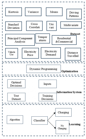
Figure 1 shows the Proposed Architecture. Various publicly available datasets on electricity costs, power demand, residential and business load profiles, temperature, and so on are currently available for use by the public [10]. As a result, there are currently only a few real-world data sets that can be used to study vehicle driving habits and no detailed data set that can be used to construct spatio-temporal models connected to the charging of a large EV fleet.
Using data from a variety of surveys, we can compute the amount of energy used, the amount of power needed, the price of electricity, and the price of gasoline. Due to the fact that we do not have all of these databases from the same city and country, since it is preferable to capture these variables in the same location where a vehicle is used, we make the following assumptions:
(1) This data set is not affected by the electricity rate.
(2) The price of electricity is closely related to the amount of electricity consumed.
For the same distance driven, gasoline costs more than electricity.
Figure 1. Proposed architecture
Data on driving habits and electricity prices collected for these studies, while not coming from the same location, provide valuable information about how Electric Vehicles handle charging. The following are the databases that were used in the experiments:
We used data available online from the Waterloo Weather Station1 to estimate the outside temperature [11]. In the Canadian city of Winnipeg, 17 different conventional vehicle GPS-based usage information was collected. Despite the fact that it does not perfectly reflect the cost of electricity for Ontarians, it is a reliable predictor of the hourly price of electricity. HOD is the total of all hourly loads from the IESO-administered market in Ontario. The HOD is calculated on a daily basis. Last but not least, the Ontario Ministry of Energy publishes weekly averages for the price of normal unleaded gasoline throughout the province. This database can be used to calculate the true cost of gas-powered transportation.
3.1 Univariate analysis
Analysis in the frequency domain and other fundamental statistical methods are the subject of univariate analysis. We quantify the central tendency and the dispersion with the mean (the first statistical moment) and the variance (the second statistical moment), respectively. The disproportion between extremes and mean is quantified by the coefficient of skewness of the sample. The histogram is perfectly symmetrical, which indicates that there is no skewness. If the skewness is positive, then more values are below the mean than above it, and if it is negative, then more values are above it. The level of peakiness in a histogram can be quantified by calculating the dimensionless sample coefficient of kurtosis (fourth statistical moment). For this purpose, we will use the number of three, which is the mean of a normal distribution [12].
In Table 1, analysis in the frequency domain and other fundamental statistical methods are the subject of univariate analysis. We quantify the central tendency and dispersion with the mean and variance, respectively. The disproportion between extremes and mean is quantified by the coefficient of skewness of the sample. The histogram is perfectly symmetrical, which indicates that there is no skewness. If the skewness is positive, then more values are below the mean than above it, and if it is negative, then more values are above it. The level of peakiness in a histogram can be quantified by calculating the dimensionless sample coefficient of kurtosis. For this purpose, we will use the number of three, which is the mean of a normal distribution [13]. Figure 2 displays the Graph of statistical values of the dataset. of the data set.
(1) Initialize the system and data sources:
· Load the data set containing electricity prices, demand, driving habits, and historical data.
· Load public facts on electricity pricing, power use, temperature, and driving behaviours.
The objective is to minimize charging costs, and knowing the real-time or predicted electricity prices is crucial. The DRL model can use these data to identify periods with lower electricity rates and recommend charging during those times. past electricity price trends, user charging habits, and historical demand in the power grid. Analyzing these data helps the DRL model predict future patterns and make informed decisions about charging schedules. It might also include past charging cycles of the specific EV to account for battery degradation and charging efficiency variations.
(2) Perform data pre-processing and analysis:
· Perform necessary data preprocessing and feature engineering.
· Handle missing values, outliers, and categorical variables.
· Normalize or scale the numerical features, if required.
· Partition of the data set into test and training sets.
· Apply univariate and multivariate analysis techniques to investigate data set complexity and gain insight.
· Explore the linear connections and periodicity between trip distances and vehicle energy use.
(3) Select a random forest machine learning algorithm for optimizing the charging strategy:
· model = RandomForestRegressor()
(4) Initialize the machine learning model with chosen hyperparameters:
· Set the model's hyperparameters learning rate.
Define the hyperparameters to tune and their possible values.
param_grid =
'n_estimators': [50, 100, 200],
'max_depth': [None, 5, 10],
min_samples_split': [2, 5, 10],
'min_samples_leaf': [1, 2, 4]
(5) Train the machine learning model:
· Fit the chosen algorithm on the training dataset.
· Adjust hyperparameters using grid search techniques.
Grid_search = GridSearchCV(estimator=model, param_grid=param_grid, cv=5)
grid_search.fit(X_train, y_train)
· Feed the input features (X_train) and target variable (y_train) to the model.
Update the model's parameters iteratively to minimize the loss or maximize the objective function.
· Apply gradient descent, backpropagation, or other optimization techniques specific to the chosen algorithm.
(6) Predict the charging strategy:
· Use the trained model to predict the optimal charging strategy based on input features such as electricity pricing, demand, driving habits, and historical data.
(7) Apply the The Principal component analysis (PCA):
· Use PCA to evaluate the variables of electricity price, demand, temperature, and distance.
· Determine the relevant aspects and preserve the data variance using PCA.
Table 1. Statistical values of datasets
|
Mean |
Standard Deviation |
Skewness |
Kurtosis |
Minimal |
Median |
Maximum |
|
5.62 |
10.26 |
-0.28 |
1.17 |
-27.55 |
6.24 |
31.2 |
Figure 2. Graph of dataset statistical values
(8) Perform clustering:
· Apply clustering techniques to reveal data set groupings and seasonal variations.
· Analyze the clustering results to understand pricing options and seasonal changes.
(9) Apply machine learning algorithms for prediction:
· Train machine learning algorithms using the dataset to predict charging trends.
· Evaluate the accuracy of the predictions.
(10) Optimize charging techniques and reduce costs:
· Utilize the predictions of the machine learning algorithms to optimize charging techniques.
· Adjust the charging strategy based on real-time trends and patterns.
(11) Evaluate the accuracy and efficiency of the system:
· Calculate evaluation metrics such as mean squared error, accuracy.
(12) Adapt to changing conditions and enhance charging efficiency:
· Utilize electricity costs, power consumption, load profiles, and temperature data to adapt the system to changing conditions.
· Enhance the charging efficiency by adjusting the charging strategy based on the seasonal charging behavior and energy use.
(13) Evaluate the system performance:
· Measure the accuracy of the system's predictions and adjustments to seasonal changes.
· Assess the reduction in charging expenses compared to traditional approaches.
Data quality and consistency, data availability and granularity, data relevance, and bias. The algorithm begins by initializing the system and loading the required data sources, including a dataset with electricity prices, demand, driving habits, and historical data, as well as public facts related to electricity prices, power use, temperature, and driving behaviors. Data pre-processing and analysis are then performed, which involves handling missing values, outliers, and categorical variables, as well as normalizing or scaling numerical features [14]. The data set is split into training and testing sets, and univariate and multivariate analysis techniques are applied to gain insights into the data set's complexity. The algorithm selects the Random Forest Regressor as the machine learning algorithm for optimizing the charging strategy. The model is initialized with chosen hyperparameters and a grid search is used to tune the hyperparameters. The model is trained on the training data set and the input features and target variable are fed to the model. The model parameters are updated iteratively to minimize loss or maximize the objective function. The trained model is then used to predict the optimal charging strategy based on the input characteristics, considering the price of electricity, demand, driving habits, and historical data. Principle Component Analysis (PCA) is applied to evaluate the variables of electricity price, demand, temperature, and distance and determine their relevance. Univariate analysis probably refers to analyzing each dataset (electricity prices, battery levels, etc.) independently. This can provide valuable information before feeding them into the DRL model. Statistical Significance: Statistical tests can determine whether the observed trends in each data set are statistically significant or simply due to random chance. This helps to identify reliable patterns from which the DRL model can learn. Insights on Individual Variables Analyzing each variable helps to understand its range, distribution, and potential outliers. For example, analyzing historical electricity prices might reveal peak and off-peak hours, informing the DRL model on cost-effective charging times.
Clustering techniques are used to identify groupings of data sets and seasonal variations, with a focus on understanding pricing options and seasonal changes [15]. Additional machine learning algorithms are trained to predict charging trends and their accuracy is evaluated. The algorithm optimizes charging techniques and reduces costs by taking advantage of predictions from machine learning algorithms and adjusting the charging strategy based on real-time trends and patterns. The system's accuracy and efficiency in sorting and recognizing trends in varied data sources are evaluated using evaluation metrics such as mean squared error and accuracy. The system adapts to changing conditions and improves charging efficiency by using electricity costs, power consumption, load profiles, and temperature data. The algorithm evaluates the system performance by measuring the accuracy of its predictions and adjustments to seasonal changes, as well as assessing the reduction in charging expenses compared to traditional approaches [16]. The algorithm provides a comprehensive framework for developing and evaluating a machine learning-based charging strategy optimization system. Overall, the algorithm encompasses the necessary steps to build and evaluate a machine learning-based charging strategy optimization system. It uses data analysis, machine learning algorithms, hyperparameter tuning, and evaluation metrics to improve charging efficiency and reduce costs in real-world scenarios.
3.2 Optimization
When an electric vehicle is plugged in, the smart charging optimization process decides what to do at when times (e.g., every 15 minutes) to maximize efficiency and minimize the owner's energy bill. Optimization is conducted using reinforcement learning. Optimization using Q learning implementation.By integrating reinforcement learning with Q learning, we can optimize the charging judgments of Electric Vehicles (EVs) at a charging station. In this scenario, the environment is the EV charging station and the agent (EV) learns when to charge to minimize costs and maximize efficiency. The goal is to determine the optimal charging policy that minimizes the cost of charging an electric vehicle (EV), taking into consideration the time-of-use electricity pricing structure and the state of charge (SoC) of the EV battery [17, 18].
State (s): The SoC of the EV's battery and the current time interval can represent the system's state.
Action (a):The action represents the charging rate or the amount of energy the electric vehicle will absorb during the current time interval.
Reward (R):The reward can be a function of the charging cost, the battery state (such as preventing overcharging or undercharging), and any other relevant factors.
Q-value function (Q(s, a)):The Q-value function represents the anticipated cumulative reward the agent will receive by taking action 'a' in state's' and subsequently adhering to the optimal policy.
Using the Q-learning update formula, the Q-value function can be updated.
$\mathrm{Q}(\mathrm{S}, \mathrm{a})=\mathrm{Q}(\mathrm{s}, \mathrm{a})+\alpha^*\left[\mathrm{R}+\gamma^*\left(\mathrm{Q}\left(\mathrm{s}^{\prime} \mathrm{a}^{\prime}\right)-\mathrm{Q}(\mathrm{s}, \mathrm{a})\right)\right]$ (1)
- Q(s, a) represents the Q value for state s' and action a'.
- is the learning rate, which determines how frequently the agent revises the Q-value in light of new experiences. It is a numeric value between 0 and 1.
- R is the immediate recompense the EV receives for performing action a in state's.
- The discount factor that determines the value of future rewards is. It is a numeric value between 0 and 1.
- max(Q(s', a')) returns the maximum Q-value for the next state's' (s') across all potential actions a.
- Q(s', a') is the Q-value for the next state's' (s') and action a' that the agent chooses in accordance with its policy.
3.3 Exploration-extraction technique
An epsilon-greedy strategy is utilized to strike a balance between investigating new charging strategies and utilizing current knowledge. The agent chooses the action with the highest Q-value with a probability of (1 - ) (exploitation) and a random action with a probability of (exploration). As the agent gains more experience and acquires more knowledge, can be lowered over time to gradually transition from protection to exploitation.
3.4 Agent
During numerous charging sessions or episodes, the agent (EV) interacts with the station's environment. Throughout each episode, the agent updates its Q values based on the environment's rewards. As training progresses, the agent progressively uses the learned Q values to make better charging decisions. Initially, the agent explores various charging strategies, but as training progresses, the agent increasingly uses the learned Q-values to make better charging decisions.
3.5 Optimization algorithm
(1) Initialize the Q value function Q(s, a) with random values.
(2) Observe the current state's'.
(3) Select an action a using the epsilon-greedy strategy.
(4) Execute action a in the charging station environment and observe the reward 'R' and the next state's'.
(5) Update the Q-value using the Q-learning update formula.
(6) Set the current state's' to the next state's'.
(7) Repeat steps 3 to 6 for multiple charging sessions.
Using reinforcement learning, Q-learning, and an exploration-exploitation strategy, an electric vehicle (EV) can learn an optimal charging policy that minimizes costs and maximizes efficiency over time [19, 20]. This enables the electric vehicle to adapt to fluctuating electricity prices and charging demands, allowing it to make better charging judgements in real-world situations.
The cost goal factor is a mathematical equation that tells you what to do when the vehicle is connected to a charging station (Sc) and when it is not (Su). The cost function is expressed as follows when the vehicle is connected:
$\mathrm{Sc}(\mathrm{t})=\mathrm{b}(\mathrm{t}) * \mathrm{c}(\mathrm{t}) * \operatorname{Ech}(\operatorname{Soc}(\mathrm{t})) * \mathrm{n}(1-\gamma)$ (2)
where, b(t) is the decision variable representing the charging action at time t (1 for charging, 0 for standby).
C(t) is the cost factor, which at time t may include the price of electricity, the demand, or other pertinent parameters.
The charging rate may vary according to the current state of the battery.
Represents the efficacy of the charging process, ranging from 0 to 1. The discount factor modifies the cost function to accommodate for special circumstances. The equation represents the cost incurred when the vehicle is turned in, taking into consideration the charging decision, electricity cost, energy supplied to the battery, charging efficiency, and any other relevant factors. It can be modified by designating specific values or incorporating additional terms in accordance with the problem's specific context and requirements. In our approach, we suggest using a straightforward threshold-based rule (TBR) that considers the electricity price and the current charge level. The threshold is computed using a sigmoid function:
$\mathrm{f}(x, a, b)=1 /(1+\exp [-a(x-b)])$ (3)
where, x represents the current charge level. a and b are parameters that can be optimized using the CMA-ES method or any other optimization technique. exp[] denotes the exponential function. The sigmoid function helps to determine the threshold on the basis of the present level of charge. The sigmoid function transitions between 0 and 1 as the charge level (x) approaches the value of the parameter b, allowing a progressive change in the decision based on the electricity price. Taking into account the objective function to be optimized, the optimized values of parameters a and b can be obtained using any applicable optimization algorithm.
Using the formula, we define a threshold rule that adapts to the current charge level and electricity price, enabling us to make decisions based on the sigmoidal relationship between these variables.
$a(t)=\left\{\begin{array}{c}1(\text { charge if cel }(t) \leq f(x, a, b) \\ 0 \cdot(\text { standby)otherwise }\end{array}\right.$ (4)
where, Cel(t) represents the normalized electricity price at time t. x represents the state of charge, SoC(t). f(x, a, b) is the sigmoid function defined as: f(x, a, b) = 1 / (1 + exp[-a(x - b)]). In this formulation, if the normalized electricity price, Cel(t), is less than or equal to the threshold calculated using the sigmoid function f(x, a, b), the decision variable a(t) is set to 1, indicating that the vehicle should be in the charging mode. Otherwise, if Cel(t) is greater than the threshold, a(t) is set to 0, indicating that the vehicle should be in standby mode. The decision rule allows adaptive charging decisions based on the interaction, enabling efficient management of the charging process.
Table 2. Total and maximum one-way distance traveled by vehicles during the evaluation window (in kilometers)
|
Summer |
Winter |
||
|
Total Distance |
Max Trip Distance |
Total Distance |
Max Trip Distance |
|
2317.09 |
14.65 |
1087.34 |
10.35 |
|
934.47 |
25.78 |
2837.21 |
16.57 |
|
1639.85 |
29.12 |
3481.95 |
20.43 |
|
2857.43 |
20.92 |
546.06 |
11.89 |
|
763.77 |
18.45 |
2359.25 |
15.28 |
|
2015.96 |
12.34 |
970.11 |
14.46 |
|
3339.07 |
21.78 |
3947.32 |
28.75 |
|
1654.2 |
16.15 |
3094.59 |
19.31 |
|
1076.45 |
29.89 |
1764.77 |
12.97 |
|
2418.11 |
17.26 |
3812.88 |
22.51 |
|
2890.98 |
22.43 |
1490.15 |
26.96 |
|
594.13 |
19.63 |
4092.75 |
18.14 |
|
3368.87 |
28.57 |
1312.25 |
13.45 |
|
1879.62 |
15.74 |
2785.39 |
17.83 |
|
4137.58 |
23.68 |
760.28 |
10.92 |
|
2191.45 |
13.97 |
2069.51 |
15.71 |
|
1278.86 |
26.41 |
3034.47 |
12.32 |
Figure 3. Total and Maximum distance travelled
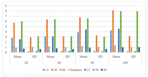
Table 3. The 17 vehicles' average improvement (in percentage) of the 17 vehicles over the standard 10-bin scheme at each t during the summer and winter training periods
|
Summer |
20 |
30 |
50 |
100 |
||||
|
X |
SD |
X |
SD |
X |
SD |
X |
SD |
|
|
15 |
2.83 |
0.2 |
3.12 |
0.25 |
3.92 |
0.27 |
4.26 |
0.22 |
|
30 |
5.76 |
2.95 |
6.41 |
3.12 |
6.84 |
3.3 |
8.15 |
3.18 |
|
60 |
0.92 |
1.08 |
1.19 |
1.04 |
1.25 |
1.05 |
1.42 |
1.03 |
|
Winter |
X |
SD |
X |
SD |
X |
SD |
X |
SD |
|
15 |
2.54 |
0.24 |
3.12 |
0.27 |
4.42 |
0.22 |
4.57 |
0.25 |
|
30 |
6.02 |
3.1 |
6.38 |
3.1 |
6.61 |
3.05 |
7.99 |
7.99 |
|
60 |
0.74 |
0.66 |
0.81 |
0.68 |
0.93 |
0.67 |
1.04 |
1.04 |
Figure 3 discusses about Total and maximum distance traveled. Table 2 shows the total and maximum one-way distance traveled by vehicles during the evaluation window (in kilometers). Table 3 summarizes the 17 vehicles' average improvement (in percentage) over the standard 10-bins scheme at each t during the summer and winter training periods.
4.1 Q Learning
Dynamic programming enables optimal decisions to be made on historical datasets because all vehicle and There is a historical record of environmental information, including projected values. Agent: the DRL model acts as the agent, making decisions about charging schedules. State (S): current situation, including factors such as battery level, electricity price, and time of day. Action (A): the possible charging decisions the agent can make, such as "charge now," "charge later," or "don't charge. Reward (R): the numerical feedback signal the agent receives based on the outcome of its action. A positive reward signifies a good decision (for example, charging during off-peak hours), while a negative reward indicates an undesirable outcome (for example, charging during peak hours). Value Q (Q (S, A)): the future estimated reward the agent expects to receive by taking action A in state S. The DRL model learns and updates these Q-values over time. Research applies dynamic programming to the tagging of historical databases in the state-space format described above. These annotated data, along with standard supervised learning algorithms, can be used to make decisions in real time, such as the optimal time to charge a car.
Figure 4 explained both summer and winter training, the average cost per bin.
Pseudocode:
Initialize Q(S, A) for all states (S) and actions (A) with a small value (e.g., 0)
Loop:
Observe the current state (S)
4.2 Dynamic programming
To formulate the Dynamic Programming (DP) model for optimizing electric vehicle (EV) charging, we define the decision model's hyperparameters. The objective is to maximize the cost savings achieved by the AC model compared to the gas-only strategy. Electric Vehicles (EVs) have gained increasing popularity due to their eco-friendly nature and potential cost savings over traditional gas-powered vehicles. Efficient charging of Electric Vehicles can significantly impact cost reduction and energy utilization. To address this challenge, we employ the dynamic programming (DP) model, a powerful technique for solving complex optimization problems.
The objective of the DP model is to maximize the cost savings achieved by employing an Always Charge (AC) strategy for EV charging. We compare this strategy with a gas-only approach, which serves as the baseline. The AC model charges the EV when parked and the battery is not full, considering electricity prices and vehicle-specific characteristics. The DP model represents the charging process as a sequence of discrete time steps. Each time step is associated with a State of Charge (SoC), which represents the battery's current energy level. The DP algorithm selects actions at each time step, determining when and how much to charge the EV, to optimize cost savings.
Figure 4. For both summer and winter training, the average cost per bin
The cost function in the DP model captures the economic impact of charging decisions. It considers factors such as electricity prices, distance traveled, and battery capacity. The goal is to minimize the overall cost of charging Electric Vehicles while ensuring sufficient energy for daily usage. The DP algorithm uses the Bellman equation, a recursive equation that expresses the value of a state as the expected sum of future rewards. In our case, the value function represents the cost savings achieved by following a specific charging strategy from a given SoC at a specific time step.
The DP algorithm starts at the final time step (e.g., end of the day) with a fully charged battery and computes the optimal cost savings for each SoC level. Then it moves back in time, calculating the cost savings at each time step based on the optimal decisions made in future time steps. This process continues until the initial time step (for example, the beginning of the day) is reached. The DP model's outputs are the optimal charging decisions for each time step, allowing the EV to achieve maximum cost savings during the day. The results demonstrate the efficiency of the AC strategy compared to that of the gas-only approach. The cost savings of the AC model are summarized in Table 4 for different EVs under various scenarios.
Table 4. Results for the models (a) Summer (b) Winter
|
(a) Summer |
|||||
|
S.No |
Season |
DNN |
KNN |
SNN |
TBR |
|
1 |
Winter |
0.95 |
0.75 |
0.9 |
0.7 |
|
2 |
Winter |
0.93 |
0.78 |
0.88 |
0.65 |
|
3 |
Winter |
0.91 |
0.8 |
0.85 |
0.68 |
|
4 |
Winter |
0.94 |
0.77 |
0.92 |
0.72 |
|
5 |
Winter |
0.96 |
0.76 |
0.89 |
0.73 |
|
6 |
Winter |
0.9 |
0.79 |
0.87 |
0.71 |
|
7 |
Winter |
0.92 |
0.74 |
0.91 |
0.69 |
|
8 |
Winter |
0.93 |
0.72 |
0.86 |
0.74 |
|
9 |
Winter |
0.95 |
0.75 |
0.93 |
0.76 |
|
10 |
Winter |
0.9 |
0.71 |
0.85 |
0.67 |
|
11 |
Winter |
0.91 |
0.79 |
0.88 |
0.68 |
|
12 |
Winter |
0.94 |
0.73 |
0.89 |
0.71 |
|
13 |
Winter |
0.93 |
0.75 |
0.91 |
0.73 |
|
14 |
Winter |
0.92 |
0.7 |
0.86 |
0.67 |
|
15 |
Winter |
0.96 |
0.78 |
0.89 |
0.75 |
|
16 |
Winter |
0.9 |
0.72 |
0.87 |
0.68 |
|
17 |
Winter |
0.91 |
0.76 |
0.88 |
0.7 |
|
(b) Winter |
|||||
|
S.No |
Season |
DNN |
KNN |
SNN |
TBR |
|
1 |
Summer |
0.97 |
0.79 |
0.93 |
0.72 |
|
2 |
Summer |
0.95 |
0.75 |
0.91 |
0.68 |
|
3 |
Summer |
0.92 |
0.8 |
0.88 |
0.69 |
|
4 |
Summer |
0.96 |
0.78 |
0.94 |
0.71 |
|
5 |
Summer |
0.98 |
0.77 |
0.92 |
0.7 |
|
6 |
Summer |
0.91 |
0.79 |
0.89 |
0.73 |
|
7 |
Summer |
0.93 |
0.76 |
0.91 |
0.71 |
|
8 |
Summer |
0.94 |
0.72 |
0.87 |
0.68 |
|
9 |
Summer |
0.97 |
0.75 |
0.93 |
0.7 |
|
10 |
Summer |
0.91 |
0.7 |
0.86 |
0.67 |
|
11 |
Summer |
0.92 |
0.78 |
0.89 |
0.68 |
|
12 |
Summer |
0.95 |
0.73 |
0.9 |
0.71 |
|
13 |
Summer |
0.94 |
0.75 |
0.92 |
0.73 |
|
14 |
Summer |
0.93 |
0.71 |
0.87 |
0.67 |
|
15 |
Summer |
0.98 |
0.79 |
0.93 |
0.75 |
|
16 |
Summer |
0.91 |
0.72 |
0.88 |
0.68 |
|
17 |
Summer |
0.92 |
0.76 |
0.89 |
0.7 |
The Dynamic Programming model proves to be a powerful tool for optimizing electric vehicle charging strategies. By incorporating various parameters and constraints, such as electricity prices, battery capacity, and travel distances, the DP algorithm effectively determines the optimal charging decisions. The AC strategy emerges as a cost-effective solution that yields substantial savings over the gas-only approach. Implementing the DP model in real-world EV charging scenarios holds great promise for sustainable and economically efficient transportation. Further research and development in dynamic optimization techniques can lead to even more advanced and environmentally friendly EV charging solutions.
4.3 Threshold-Based Rule (TBR) for electric vehicle charging optimization
In our approach to optimize Electric Vehicle (EV) charging decisions, we propose using a simple Threshold-Based Rule (TBR) based on the present charge level of the EV's battery and the price of electricity. Using a sigmoid function that computes a threshold value, the TBR determines whether the EV should be in charging mode or in standby mode.
The sigmoid function, denoted as f(SoC, p1, p2), is given by the following formula.
$f(S o C, p 1, p 2)=\frac{1}{(1+\exp [-p 1(S o C-p 2)])}$ (5)
p1 and p2 are parameters that must be optimized using the CMA-ES (Covariance Matrix Adaptation Evolution Strategy) method. The SoC represents the current state of charge of the EV battery. Equation 3 defines the objective function to optimize these parameters.If Cel(t) is less than f(SoC(t), p1, p2), the electric vehicle will be charging mode (a(t) = 1). If Cel(t) is greater than f (SoC (t), p1 and p2), the EV will enter standby mode (a(t) = 0).
To derive the TBR policy, we first examine the sigmoid function f(SoC, p1, p2). The sigmoid function converts the value of the SoC to a number between 0 and 1. When SoC approaches p2, f(SoC, p1, p2) approaches 0.50. As SoC increases or decreases relative to p2, f(SoC, p1, p2) approaches 1 or 0 respectively.
In the charging decision formula, the normalized electricity price Cel(t) is compared with f (SoC (t), p1, p2) using the Cel(t) normalization factor. If Cel(t) is less than or equal to f(SoC(t), p1, p2), it indicates that the price of electricity is relatively low or within an acceptable range, and charging the electric vehicle is cost-effective. The electric vehicle will be set to charging mode (a(t) = 1) in this case.
Alternatively, if Cel(t) is greater than f(SoC(t), p1, p2), it indicates that the price of electricity is relatively high and it may be more cost-effective to refrain from charging the electric vehicle. Consequently, the EV will enter standby mode (a(t) = 0).
The parameters of the sigmoid function p1 and p2 are optimized using the CMA-ES method, which iteratively searches for the values that result in the greatest performance. This optimization process enables the TBR policy to adapt to various charging scenarios and achieve a cost-effective and efficient charging strategy for the electric vehicle.
4.4 k-NN to optimize electric vehicle charging
We employ the k-NN algorithm in our approach to optimizing electric vehicle (EV) charging decisions. Let S represent the state of the EV and A represent the action (charge or standby) performed by the EV in that state. The k-NN algorithm is implemented as follows:
· Define a distance metric, such as the Euclidean distance, to quantify the degree of similarity between states. Smaller distances indicate greater similarity between governments.
· Create the training dataset, which consists of pairs (S_i, A_i) in which S_i represents the state and A_i is the action conducted in that state. Using dynamic programming to determine the optimal charging decisions for various states yields the training dataset.
· Given a new state S, using the defined distance metric, locate the k nearest neighbors in the training data set. The k nearest neighbors are the k states in the training data set with the shortest distance from the newly introduced state S.
· Determine the action A for the new state S based on the majority vote of its k closest neighbors. If the preponderance of the k closest neighbors are in charging mode, the new state S will be assigned to the charging action. If not, it will be delegated to the standby action.
Through cross-validation, the optimal number of neighbors k for the k-NN algorithm is determined. Cross-validation is a technique used to evaluate the performance of an algorithm by dividing training and test datasets into numerous subsets.
Deriving k-NN for EV Charging Optimization: The k-NN algorithm for EV charging optimization is derived from the classification principles underlying the dynamic programming approach to charging decisions. Using the results of dynamic programming to construct the training dataset, the k-NN algorithm capitalizes on the knowledge of optimal charging actions for various states.
When encountering a new state S, the k-NN algorithm identifies its k nearest neighbours in the training data set. These neighbouring states have exhibited comparable taxation practices in the past. The algorithm allocates the new state to the most probable charging action by taking the majority vote of the charge/standby actions of these neighbours.
Then cross-validation is used to evaluate the efficacy of the k-NN algorithm and determine the optimal value of k. Cross-validation identifies the optimal k-value for optimal charging decisions and the overall optimization of electric vehicle charging operations by evaluating the algorithm in different subsets of the training data set.
4.5 Small neural network with clustering and feature selection
In our approach to optimize Electric Vehicle (EV) charging decisions, we suggest a two-layer SNN that takes advantage of both clustering and feature selection. The output layer is linear, while the hidden layer uses a sigmoid transfer function. The network is taught to function by employing the Levenberg-Marquardt algorithm.
We start by using clustering to pick a small but fairly representative subset of the data in the data set. The clustering method collects data points that share similarities and then reduces the resulting dataset, making it easier to train the neural network.
To further improve the SNN's performance, we employ a sequential step-by-step procedure called Backward Greedy Selection to eliminate variables (features) that either degrade or do not substantially improve the neural network's performance. The goal of this feature selection procedure is to keep only those characteristics useful for making a price determination.
First, the sigmoid transfer function () is defined for the SNN's hidden layer as follows:
$\sigma(x)=\frac{1}{(1+\exp (-x))}$ (6)
Here, x represents the input to the hidden layer, which is the weighted sum of the inputs from the previous layer.
4.5.1 Linear output function
The linear output function preserves the weighted sum of the inputs from the hidden layer without applying any activation function, making it suitable for regression tasks.
4.5.2 Levenberg-Marquardt Algorithm
The Levenberg-Marquardt algorithm is used to train the SNN. It is an optimization algorithm commonly employed for nonlinear least-squares problems. The algorithm minimizes the difference between the predicted network output and the actual target output by adjusting the weights during training.
The Backward Greedy Selection is a feature selection method that iteratively removes less informative features from the data set to enhance the performance of the neural network. The process involves the following steps:
· Start with the complete set of features.
· Train the SNN on the dataset with all the features included.
· Evaluate the SNN's performance.
· Remove the least significant feature (based on some performance metric) from the dataset.
· Retrain the SNN with the reduced set of features.
· Repeat steps 3 to 5 until the desired level of performance improvement is achieved or a stopping criterion is met.
4.6 DNN to optimize the charging of Electric Vehicles
DNN offer the advantage of learning a hierarchical representation of the data, in contrast to shallow neural networks SNN Learning complicated associations from a wide range of interdependent variables is made possible by the hierarchical structure represented by a deep neural network's layers of neurons. Due to the high correlational strength, DNNs are particularly suited to investigate the strong correlation found in our complex dataset, which includes data from all cars.
A total of 508 input neurons, four hidden layers of 256, 96, 64, and 32 neurons, and a single output neuron representing the charging action (a(t)) make up the DNN architecture. Activation Functions: Each layer's activation function is the Exponential Linear Unit (ELU), except for the output layer, which uses the softmax function. The ELU activation function is selected due to its ability to effectively manage negative inputs and mitigate the vanishing gradient problem during training, thereby enabling faster and more stable convergence.
Batch Normalization: To further promote convergence and prevent internal covariate shift, after each entirely connected layer, a batch normalization operation is added. By normalizing each batch's input during training, batch normalization stabilizes the training process and enables the network to acquire knowledge more efficiently.
The DNN is trained using the adaptive stochastic gradient descent (Adagrad) method. During training, Adagrad modifies the learning rate for each parameter based on the historical gradients of that parameter. This adaptability enables Adagrad to enhance and accelerate convergence, particularly when working with sparse data.
The ELU is a unit of length that is proportional to the exponent.
For a given input x, the activation function of the ELU is defined as follows:
$E L U(x)=x$, for $x \geq 0$, for $x<0$ (7)
x is a hyperparameter that determines the function's slope for negative inputs.
The softmax function is used to convert the logits (raw outputs) of the previous layer into a probability distribution in the output layer. The softmax function for a given vector z is defined as
$\operatorname{softmax}\left(z_{-} i\right)=\exp \left(z_{-} i\right) / \sum\left(z_{-} j\right)$ for all $j$ (8)
The output of the i-th neuron in the output layer is represented by z_i. exp denotes the exponential function. z_i is the i-th element of the input vector z.
The sum in the denominator runs over all elements z_j of the input vector z.
5.1 Always charge model
The research compares the cost savings achieved by three distinct charging strategies for Electric Vehicles: an AC model (Assumption: Vehicle charges when parked and battery is not full), an optimal charging strategy using DP and a gas-only strategy. The results are summarized in Table 4, which shows the cost of each vehicle in each of the three scenarios and the savings in relation to the cost of petroleum. Summer Cost Savings: The AC model achieves considerable cost savings in the summer, ranging from 28% to 74% across vehicles.
The simple AC strategy demonstrates remarkable efficiency, obtaining median gains of 68% in the summer and 56% in the winter, respectively. Low electricity prices on the market significantly reduce the total energy cost of Electric Vehicles, rendering the AC strategy cost-effective even when charging during peak electricity prices. The DP-based optimal charging strategy obtains impressive summer and winter median gains of 95% and 88%, respectively. This indicates that additional improvements can be made to close the disparity between AC and DP strategies, bringing the cost savings closer to the optimal benchmark. The article concludes by highlighting the potential for significant cost savings in electric vehicle charging via the AC paradigm, particularly during the summer months. However, to match the efficacy of the DP-based optimal charging strategy, further development is required. Implementing more advanced optimization techniques could result in greater cost savings and a more efficient use of available energy resources for Electric Vehicles. Supervised learning models are highly dependent on the quality and relevance of training data. Reinforcement learning can be computationally expensive and might require extensive training time.
5.2 Machine learning models
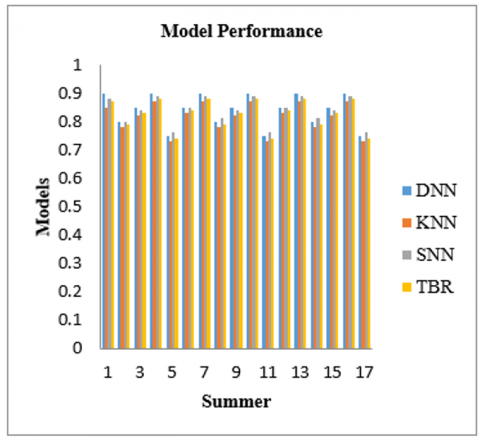
In this article, we compare the optimal pricing decisions acquired by dynamic programming (DP) with those obtained via several machine learning (ML) models. Figure 5 shows the ratio of ML model savings to DP model savings, with values close to 1 reflecting efficiency levels that are comparable to the global optimum achieved with DP. Performance of ML Models: The DP-based optimal charging method is the global optimum, but it is unworkable in practice since it demands perfect knowledge of the future. On the other hand, ML models offer effective pricing choices even when no further data is available. Metrics like the Mean Squared Error (MSE) can assess the accuracy of predicted charging schedules compared to actual optimal schedules (known from simulations or historical data). Additional metrics might include cost savings achieved, reduction in peak grid demand, and user satisfaction for a more holistic evaluation.
(a)
(b)
Figure 5. Model gain for two seasons (a) Summer (b) Winter
DNN performs better: The Deep Neural Network (DNN) method achieves outstanding results, with a gain ratio of 0.95 being typical. The DNN model is promising for optimizing EV charging, as it can be easily implemented in practical, real-world circumstances. Promising Actors: The average ratios for the summer and winter sessions are 0.88 and 0.80, respectively, demonstrating the efficacy of other methods such as shallow neural networks (SNN). This demonstrates that even a low-capacity model may be efficiently implemented with a thorough preselection of input variables, allowing the creation of driving habits and regular driving schedules, which are crucial for charge decisions. The KNN and TBR Approaches: When comparing summer and winter gain ratios, the K-Nearest Neighbors (KNN) and Threshold-Based Rule (TBR) methods score 0.77 and 0.72, respectively. Even though they cannot compare to the effectiveness of DNN and SNN, they outperform rudimentary methods like the AC model by a wide margin.
The evaluation indicates that the DNN approach is a standout performer among the ML models, closely approaching the global optimum found with DP. The SNN method also shows strong performance, and both models are viable alternatives to DP, given their operational suitability in real-world scenarios. Even with lower-capacity models like KNN and TBR, substantial efficiency gains are achieved compared to simple strategies such as the AC model. The findings suggest that ML-based charging strategies have great potential for cost savings and efficient energy utilization in electric vehicle charging operations.
Mean squared error (MSE): this metric measures the average squared difference between the predicted charging schedule and the actual optimal schedule (known from simulations or historical data). Lower MSE indicates better model accuracy. accuracy: This metric, when applicable (e.g., classifying peak vs. off-peak hours), represents the proportion of correct predictions made by the model. Cost savings: this metric directly measures the financial benefit achieved through optimized charging compared to a baseline strategy (e.g., always charging). Grid demand reduction: this metric quantifies the decrease in peak grid demand by optimizing charging schedules, contributing to grid stability.
Optimize charging schedules for Electric Vehicles (EVs) to minimize costs and improve efficiency. Compared three charging strategies: Always Charge (AC), optimal charging with Dynamic Programming (DP), and gas only. Evaluated several machine learning (ML) models to predict optimal charging times. These included Deep Neural Networks (DNNs), Support Vector Machines (SVMs), K-Nearest Neighbors (KNNs), and Time-Based Rules (TBRs). Analyzed correlations between factors such as time of day (HOD), hour of parking end (HOEP), temperature, gas price and distance traveled. Reduce EV charging costs compared to gasoline vehicles. Improve the efficiency of electric vehicle charging by leveraging historical data and predictions. he AC model achieved significant cost savings (28% to 74%) during the summer due to lower electricity prices. The DP model achieved even greater savings (95% summer, 88% winter) but requires unrealistic knowledge of future electricity prices. The DNN model showed promise, achieving near-optimal performance (0.95 mean gain ratio) and is suitable for real-world implementation. Other ML models, such as SVM, KNN, and TBR, also offered cost savings compared to AC. Multivariate analysis revealed correlations between factors such as HOD, HOEP, temperature, gas price, and distance traveled. These factors are important to predict optimal charging times. The limited size of the data set might affect the generalizability of the findings. DP's requirement for perfect future knowledge makes it impractical for real-world use. Explore even larger and more diverse datasets to improve model robustness. Investigate new algorithms, particularly deep learning architectures, to potentially surpass DNN performance. Integrate user preferences for charging times and locations into the optimization process. Deploy the system in a real-world setting to assess its effectiveness with actual users.
[1] Msaddek, H., Mansouri, A., Trabelsi, H. (2023). Optimal design and cogging torque minimization of a permanent magnet motor for an electric vehicle. Tehnički vjesnik, 30(2): 538-544. https://doi.org/10.17559/TV-20220815140808
[2] Tamilvizhi, T., Surendran, R., Krishnaraj, N. (2021). Cloud based smart vehicle tracking system. In 2021 International Conference on Computing, Electronics & Communications Engineering (iCCECE), Southend, United Kingdom, pp. 1-6. IEEE. https://doi.org/10.1109/iCCECE52344.2021.9534843
[3] Campaña, M., Inga, E. (2023). Optimal planning of electric vehicle charging stations considering traffic load for smart cities. World Electric Vehicle Journal, 14(4): 104. https://doi.org/10.3390/wevj14040104
[4] Shahriar, S., Al-Ali, A.R., Osman, A.H., Dhou, S., Nijim, M. (2020). Machine learning approaches for EV charging behavior: A review. IEEE Access, 8: 168980-168993. https://doi.org/10.1109/ACCESS.2020.3023388
[5] Kumar, K.R., Saravanan, M.S., Surendran, R. (2023). A novel method to predict sales price of domestic vehicles using news sentiment analysis with random forest algorithm. In 2023 2nd International Conference on Applied Artificial Intelligence and Computing (ICAAIC), Salem, India, pp. 761-765. https://doi.org/10.1109/ICAAIC56838.2023.10141389
[6] Mukherjee, J.C., Gupta, A. (2014). A review of charge scheduling of Electric Vehicles in smart grid. IEEE Systems Journal, 9(4): 1541-1553. https://doi.org/10.1109/JSYST.2014.2356559
[7] Dran, S., Varthini, P. (2013). Detecting power systems failure based on fuzzy rule in power grid. Przegląd Elektrotechniczny, 89(8): 172-177.
https://www.infona.pl/resource/bwmeta1.element.baztech-4b475d71-8aca-4b8d-9c1a-47dfbb5a3c50
[8] Adil, M., Mahmud, M.P., Kouzani, A. Z., Khoo, S.Y. (2024). Optimal location and pricing of electric vehicle charging stations using machine learning and stackelberg game. IEEE Transactions on Industry Applications, 60(3): 4708-4722. https://doi.org/10.1109/TIA.2024.3364579
[9] Azzouz, I., Fekih Hassen, W. (2023). Optimization of Electric Vehicles charging scheduling based on deep reinforcement learning: A decentralized approach. Energies, 16(24): 8102. https://doi.org/10.3390/en16248102
[10] Chung, Y.W., Khaki, B., Li, T., Chu, C., Gadh, R. (2019). Ensemble machine learning-based algorithm for electric vehicle user behavior prediction. Applied Energy, 254: 113732. https://doi.org/10.1016/j.apenergy.2019.113732
[11] Raveena, S., Surendran, R. (2023). Clustering-based hemileia vastatrix disease prediction in coffee leaf using deep belief network. In 2023 8th International Conference on Communication and Electronics Systems (ICCES), Coimbatore, India, pp. 1094-1100. https://doi.org/10.1109/ICCES57224.2023.10192835
[12] Chiş, A., Lundén, J., Koivunen, V. (2016). Reinforcement learning-based plug-in electric vehicle charging with forecasted price. IEEE Transactions on Vehicular Technology, 66(5): 3674-3684. https://doi.org/10.1109/TVT.2016.2603536
[13] Selvanarayanan, R., Rajandran, S., Alotaibi, Y. (2023). Using hierarchical agglomerative clustering in e-nose for coffee aroma profiling: Identification, quantification, and disease detection. Instrumentation Mesure Métrologie, 22(4): 127-140. https://doi.org/10.18280/i2m.220401
[14] Naresh, V.S., Ratnakara Rao, G.V., Prabhakar, D.V.N. (2024). Predictive machine learning in optimizing the performance of electric vehicle batteries: Techniques, challenges, and solutions. Wiley Interdisciplinary Reviews: Data Mining and Knowledge Discovery, e1539. https://doi.org/10.1002/widm.1539
[15] Golsefidi, A.H., Hüttel, F.B., Peled, I., Samaranayake, S., Pereira, F.C. (2023). A joint machine learning and optimization approach for incremental expansion of electric vehicle charging infrastructure. Transportation Research Part A: Policy and Practice, 178: 103863. https://doi.org/10.1016/j.tra.2023.103863
[16] Ullah, I., Liu, K., Yamamoto, T., Shafiullah, M., Jamal, A. (2023). Grey wolf optimizer-based machine learning algorithm to predict electric vehicle charging duration time. Transportation Letters, 15(8): 889-906. https://doi.org/10.1080/19427867.2022.2111902
[17] Vaiyapuri, T., Shankar, K., Rajendran, S., Kumar, S., Acharya, S., Kim, H. (2023). Blockchain assisted data edge verification with consensus algorithm for machine learning assisted IoT. IEEE Access, 11: 55370-55379. https://doi.org/10.1109/ACCESS.2023.3280798
[18] Shibl, M., Ismail, L., Massoud, A. (2021). Electric Vehicles charging management using machine learning considering fast charging and vehicle-to-grid operation. Energies, 14(19): 6199. https://doi.org/10.3390/en14196199
[19] Alshammari, A., Chabaan, R.C. (2023). Metaheruistic optimization based ensemble machine learning model for designing detection coil with prediction of electric vehicle charging time. Sustainability, 15(8): 6684. https://doi.org/10.3390/su15086684
[20] Gatica, G., Ahumada, G., Escobar, J.W., Linfati, R. (2018). Efficient heuristic algorithms for location of charging stations in electric vehicle routing problems. Studies in Informatics and Control, 27(1): 73-82. https://doi.org/10.24846/v27i1y201808