Mahsup*![]() | Putri Ayu Febriani | Syaharuddin
| Putri Ayu Febriani | Syaharuddin![]() | Vera Mandailina | Abdillah
| Vera Mandailina | Abdillah![]() | Ibrahim
| Ibrahim
© 2024 The authors. This article is published by IIETA and is licensed under the CC BY 4.0 license (http://creativecommons.org/licenses/by/4.0/).
OPEN ACCESS
This research aims to compare the accuracy levels of the Least Square Support Vector Machine (LS-SVM) method and its modification with other algorithms in predicting various types of data. A quantitative approach with meta-analysis was employed, and the data were analyzed using JASP software, focusing on Mean Absolute Percentage Error (MAPE), Effect Size (ES) values, and Summary Effect (SE). The data analysis concludes that, overall, the LS method exhibits an accuracy rate of 92.7%, categorized as high, with an estimated coefficient value of 0.073. Based on the algorithm used, the analysis results with the LS method achieved an accuracy rate of 87.5%. The LS-SVM method demonstrates a higher accuracy level, reaching 95.4%, while the LS-Combination method attains the highest accuracy rate, namely 95.6%. In data classification, the analysis results indicate the highest accuracy level in economic and trade data, amounting to 95.6%. For social and demographic data, the coefficient value is 0.122 with an accuracy rate of 87.8%. Finally, in agricultural and mining data, the generated accuracy rate is 86.6%. These findings provide valuable insights into the performance of the LS method and its modifications with other algorithms in the context of forecasting various types of data.
accuracy level, algorithm modifications, forecasting, the least squares method
Forecasting is a crucial aspect of conducting predictive analysis [1]. According to Taylor & Letham [2], forecasting is a common task in the field of data science that aids organizations in capacity planning, goal setting, and anomaly detection. Moran et al. [3] assert that forecasting involves the ability to predict future occurrences based on the analysis of past and current data. On the other hand, prediction is a broader concept, referring to assigning a probability distribution to an outcome based on model estimates, applicable to both realized and unrealized outcomes [4].
The Least Squares (LS) method is commonly employed for estimating coefficients in regression models [5]. According to Fujii [6], the LS method is one statistical approach used to estimate correlations among various data sets. Meanwhile, Sulaimon Mutiu [7] asserts that the LS method serves as a standard approach in regression analysis for solving over-determined system approximation, wherein there are more equations than unknowns. The LS method proves valuable in analyzing experimental data to summarize the effects of factors and test linear contrasts among predictions [8]. Furthermore, according to Kong et al. [9], the LS method is a way to find the best-fitting function by minimizing the total sum of squared errors between measured points and the corresponding straight line. Consistent with Abazid et al. [10], the LS method finds widespread application in data fitting, aiming for the best fit that minimizes the sum of squared residuals.
Research on the LS method has been applied across various domains for economic data forecasting, such as business cycle data [11], carbon price [12-15], and stock price estimation [16]. Additionally, studies employing the LS method are prevalent in predicting shallow landslides induced by rainfall [17], streamflow forecasting [18, 19], and groundwater surface elevation forecasting [20]. Su et al. [21] utilized the Least Square Regression Boosting (LSBoost) method in their research on natural gas price forecasting, obtaining low MSE and RMSE values of 1.12% and 1.06%, respectively. Furthermore, findings from a study on predicting cow dung pyrolysis for biochar production indicated that the LS-SVM model outperformed the ANN model with R2 values of 0.96 and 0.80, respectively [22].
Furthermore, the application of the LS method is widespread in climate data analysis, including wind energy data [23, 24] and air humidity data [25]. Utilizing LS in forecasting hourly fluctuations in the Air Quality Index (AQI) achieved an accuracy level of 93.24%, signifying a remarkably high precision [26]. In their study on monthly temperature estimation using the Partial Least Square (PLS) method, Ertaç et al. [27] reported an RMSE value of 1.80% and a high accuracy level of 94%. Moreover, the LS method finds application in forecasting endeavors in the United States and Europe, including the USA [28-32], the Netherlands [33, 34], Germany [35, 36], and Brazil [37]. In Peña-Guzmán et al. [38] research on forecasting water demand in residential, commercial, and industrial areas using LS-SVM, an accuracy level of 98% and a percentage error below 12% were achieved, indicating a high level of precision.
The LS method yields superior results and presents reasonable long-term elasticity concerning natural resource demand for energy consumption forecasts [39]. The LS method is extensively employed in forecasting in Asia, including China [40-44], Turkey [45], and Korea [46, 47]. Additionally, the integration of the LS method with other approaches in the forecasting domain is prevalent. Examples include LS-SVM for river flow prediction [48], Multi-Task Learning and LS-SVM for electricity load forecasting [49], LS Support Vector Machine Coupled with Data-Preprocessing Techniques (LSSVM-DWA) for river flow forecasting, Volterra-LS Support Vector Machine Model Combined with Signal Decomposition (EMD-LMD-LSSVM-Volterra) for hourly solar radiation forecasting [50], Fuzzy Clustering and Least Square Support Vector Machine Optimized with Wolf Pack Algorithm (FC-WPA-LSSVM) for short-term load forecasting at electric bus charging stations [51], and Least Square Support Vector Machine, Deep Belief Network, Singular Spectrum Analysis, and Locality-Sensitive Hashing (LSSVM-DBN-SSA-LSH) for wind power estimation [52]. Research outcomes by Tien Bui et al. [53] indicate that the predictive strength of LSSVM-BC surpasses that of SVM, achieving an accuracy rate of 93.8% in predicting landslides due to rainfall. The IGA-LS-SVM algorithm utilized by Lin et al. [54] provides a more significant MSE value of 0.83%, making it suitable for short-term power load prediction.
Numerous studies on the application of the LS method, either standalone or in combination with various algorithms, have yielded diverse accuracy levels. Earlier research findings indicate that the LS method, combined with algorithms such as Support Vector Machine (SVM), fuzzy logic, Gravitational Search Algorithm (GSA), Genetic Programming (GP), Evolutionary Seasonal Decomposition (ESD), and Signal Decomposition (SD), achieves high accuracy levels based on Mean Absolute Percentage Error (MAPE) values. However, to date, there has been a lack of focus on accuracy levels based on MAPE values. The combination of the LS method with other techniques also impacts the number of iterations, training duration, and testing of data. Therefore, the author has undertaken data collection to discuss the research outcomes of the LS-SVM method, both in its standalone form and in combination with other algorithms. The objective of this research is to assess the comparative accuracy levels of the LS method and its modifications across various types of forecasted data. This research aims to provide a deeper understanding of the effectiveness of the LS-SVM method and its modifications in forecasting various types of data. Consequently, this study not only makes a practical contribution to selecting the optimal algorithm for time series forecasting but also strengthens the theoretical foundation in the development of more advanced forecasting techniques. The anticipated in outcome of this research is an improvement in prediction accuracy, which in turn is expected to yield significant benefits in decision-making processes.
This research adopts a quantitative approach utilizing meta-analysis to delve into the error rates of the LS, LS-SVM, and the combination of LS with other algorithms in various forecasting domains such as economics, industry, social sciences, demography, agriculture, and mining. Typically, the classification function of LS-SVM can be formulated as follows [55]:
$f(x)=\operatorname{Sign}\left(W^T \varphi(x)+b\right)$ (1)
where, $\varphi(\mathrm{x})$ is referred to as a nonlinear function mapping from the input space $\mathrm{X}$ to a high-dimensional feature space. The coefficients $\mathrm{w}$ and $\mathrm{b}$ are obtained by minimizing the upper bound of the generalization error. Thus, Eq. (1) can be derived by solving the following optimization problem:
$\begin{gathered}\min \frac{1}{2} w^T w+\frac{1}{2} \gamma \sum_{i=1}^l \xi_l^2 \\ \text { s. t. } y_i=w^T \varphi\left(x_i\right)+b+\xi_i,(i=1,2, \ldots, l)\end{gathered}$ (2)
where, $\xi_i$ is the error variable and $\gamma$ is the penalty parameter. By employing the Lagrangian function and Karush-KuhnTucker (KKT) conditions for optimality in Eq. (2), we can derive the final classification solution of the primal problem as follows:
$f(x)=\operatorname{Sign}\left(\sum_{i=1}^l w_i K\left(x, x_i\right)+b\right)$ (3)
In Eq. (3), K represents the kernel function, which serves to simplify the utilization of mapping. The research methodology, illustrated in Figure 1, outlines the procedural steps undertaken in this study.
Figure 1. Research procedure
The data collection process involved searching for relevant research findings in both national and international indexed databases. Inclusion criteria encompassed studies conducted between 2013-2023, employing keywords such as “Prediction, Forecasting, LS, LS-SVM”, and featuring statistical data including data volume and accuracy parameters (MAD, MSE, MAPE, or RMSE). Conversely, exclusion criteria targeted quantitative studies and articles available only in full text. All relevant articles were downloaded and stored in a designated folder. In the second phase, each article was reviewed to ascertain (1) the input data size (N) during prediction, training, or testing stages, and (2) the value of Mean Absolute Percentage Error (MAPE). Subsequently, coding and tabulation were conducted, encompassing (1) publication year; (2) author names; (3) type of forecasted data; (4) country; (5) forecasting method (LS); (6) data size (N); and (7) Mean Absolute Percentage Error (MAPE) values. The accuracy criteria for MAPE, as outlined by Yadav and Nath [56], are presented in Table 1.
Table 1 presents criteria indicating the accuracy level based on Mean Absolute Percentage Error (MAPE) values to classify whether forecast outputs can be accepted or rejected. MAPE values <10% indicate highly accurate forecasting, 10% < MAPE <20% denotes good forecasting, 20% < MAPE <50% suggests acceptable forecasting, and MAPE >50% indicates inaccurate forecasting. Subsequently, Mean Absolute Percentage Error (MAPE) values were transformed into effect size (ES), and finally, ES values were converted into summary effect (SE) using the following formula:
Table 1. Criteria for MAPE value
|
Percentage |
Decimal |
Category |
|
<10% |
<0.1 |
Very accurate |
|
10%≤ MAPE<20% |
0.1≤ MAPE<0.2 |
Accurate |
|
20%≤ MAPE<50% |
0.2≤MAPE<0.5 |
Worthy |
|
≥50% |
≥0.5 |
Not accurate |
$E S=0.5 \times L N\left(\frac{1+M A P E}{1-M A P E}\right)$ (4)
$S E=\sqrt{\frac{E S(1-E S)}{N}}$ (5)
Next, the data is tabulated in Microsoft Excel and saved in CVS (Macintosh) format. The stored data is then uploaded to the JASP software for coefficient determination, rank p-value testing, and forest plot generation. The output from JASP is interpreted to assess the accuracy level based on the MAPE values pf the Least Square method in forecasting, both overall and when employing conventional and combined methods. Finally, conclusions are drawn based on the conducted analysis.
3.1 The search result
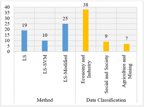
A total of 140 data points were collected for the study, with 54 meeting the specified criteria. There were 19 articles on the LS method, 10 articles on the LS-SVM method, and 25 articles on the LS method combined with other algorithms. The distribution of data is illustrated in Figure 2 and Figure 3.
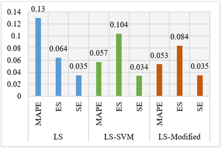
Based on the analysis of Figure 2 and Figure 3, the data analysis results reveal the utilization of three classification intervals for data forecasting: LS method, LS-SVM method, and LS modification with other algorithms. The LS method demonstrates commendable performance with 19 data points, exhibiting an average Mean Absolute Percentage Error (MAPE) of 0.13, an average Effect Size (ES) of 0.064, and an average Standard Error (SE) of 0.035, categorizing it as highly proficient.
Figure 2. Data quantity based on method and data classification
Figure 3. Average values of MAPE, ES, and SE based on method classification
In the LS-SVM method, based on dataset of 10 entries, the average MAPE stands at 0.057, with an average ES of 0.104 and an average SE of 0.034, also falling within the excellent category. Meanwhile, the LS method combine with other algorithms showcases outstanding performance, yielding an average MAPE of 0.053, an ES of 0.084, and an SE of 0.035, leveraging a dataset of 25 entries. Furthermore, the data is categorized into three intervals: economic and industrial (38 data points), social and demographic (9 data points), and agricultural and mining (7 data points). The MAPE values for each data point are delineated in Figure 4.
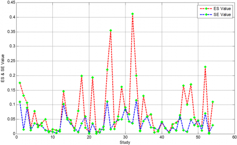
In Figure 4, the analysis results indicate that the average Mean Absolute Percentage Error (MAPE) value reaches 0.081, signifying a remarkably high level of accuracy in forecasting. Furthermore, the data reveals that the minimum recorded MAPE value is 0.001, while the maximum value reaches 0.412. This information serves as an indicator of the model's reliability, considering that lower MAPE values correspond to more accurate forecasts. The subsequent step involves determining the values of effect size (ES) and standard error (SE) based on MAPE values and the number of data points (N), as illustrated in Figure 5.
3.2 Homogeneity test and publication bias test
Based on the ES and SE values of each dataset, the data were processed using JASP software to determine the category of the method employed (Fixed Effect or Random Effect model), coefficients, p-value rank test values, and funnel plot to ascertain the average error rate based on the predetermined model. The resulting JASP output can be found in Tables 2-4.
Table 2. Fixed and random effect
|
|
Q |
df |
p |
|
Omnibus test of model coefficients |
35.816 |
1 |
<.001 |
|
Test of residual heterogeneity |
1290.756 |
53 |
<.001 |
Figure 4. Summary of MAPE values
Figure 5. Values of ES and SE for each data point
Table 3. Coefficients
|
|
|
|
|
|
95% Confidence Interval |
|
|
|
Estimate |
Standard Error |
z |
p |
Lower |
Upper |
|
Intercept |
0.073 |
0.012 |
5.985 |
<.001 |
0.049 |
0.097 |
Table 4. p-value of rank correlation
|
Rank Correlation Test for Funnel Plot Asymmetry |
||
|
|
Kendall's τ |
p |
|
Rank test |
0.222 |
0.019 |
According to Table 2, the obtained information indicates that the input data fall into the heterogeneous category, with a residual heterogeneity test value of 1,290.756 and a significant variation among the data, indicating the complexity in the characteristics of the dataset used. Furthermore, from Table 3 an estimation coefficient value of 0.073 with a significant p-value < 0.001 is obtained for the LS method. This illustrates that the LS method demonstrates a low level of error in predicting or forecasting data, affirming the reliability of this method in predictive analysis. Meanwhile, in Table 4 the p-value of rank correlation is found to be 0.019 > 0.001, indicating no indication of publication bias within the dataset utilized. Thus, the data from the 54 articles included in the study are deemed sufficiently representative to draw conclusions from this research, without significant influence from publication bias.
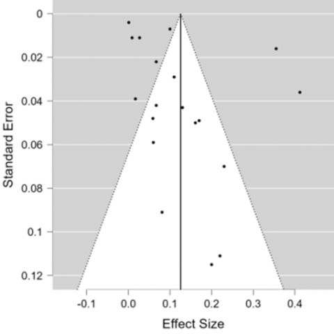
In Figure 6, the JASP software output reveals that the funnel plot of the overall data indicates no research bias, marked by all circles enclosed or declared as not indicating publication bias. In other words, the results of the p-Rank test < α = 0.05 suggest no indication of bias, as seen in Table 4. The forest plot value is 0.07 [0.05, 0.10], indicating an error rate of 7.3%, thus demonstrating an overall accuracy level of 92.7% for the LS method. Subsequently, the author divides the data based on the classification of methods and algorithms used. The JASP outputs based on these classifications are presented in Table 5.
Figure 6. Funnel plot of overall data
Table 5. MAPE category
|
Method |
N |
Estimate |
Category of MAPE |
Z |
p |
Forest Plot |
Accuracy Level |
|
|
LS |
19 |
0.125 |
12.5% |
Accurate |
4.478 |
<.001 |
0.13 [0.07, 0.18] |
87.5% |
|
LS-SVM |
10 |
0.046 |
4.6% |
High Accurate |
2.191 |
0.028 |
0.05 [0.00, 0.09] |
95.4% |
|
LS-Combination |
25 |
0.044 |
4.4% |
High Accurate |
4.455 |
<.001 |
0.04 [0.02, 0.06] |
95.6% |
From the results in Table 5, it is evident that the error rate for the LS method with N = 19 is 13% (0.07-0.18), and the estimated value is 0.125 with a p-value < 0.001, signifying an accuracy level of 87.5%. Furthermore, the error rate for LS-SVM with N = 10 yields a result of 4.6% (0.00-0.09), an estimated value of 0.046, and a p-value of 0.028 < 0.05, indicating that LS-SVM has an accuracy level of 95.4%. This aligns with the research by Sun and Liang [57], where short-term electricity load forecasting using LS-SVM achieved a low MAPE value of 2.34%. However, in the research conducted by Biswas et al. [58], experimental result indicate that the performance of the MARS model slightly outperforms that of the LS-SVM model. For LS-Combination with N = 25, the error rate is 4.4% (0.02-0.06), the estimated value is 0.044, and the p-value is < 0.001, implying that LS-Combination also has an accuracy level of 95.6% in predicting data. Consistent with the findings of Niu and Dai [59], the proposed short-term load forecasting model with EMD-GRA-MPSO-LS-SVM outperforms other models with a MAPE value of 1.1%. In contrast to the study by Yang et al. [60] utilizing the PLSE-RVM method, where the accuracy rate reached 63.3%. The distribution pattern can be observed in Figure 7.
From the JASP output, it is evident that the plot trajectories of the three algorithms indicate no indication of publication bias, as marked by the absence of open circles, meaning no missing studies. Additionally, all circles are enclosed, signifying that the research sample meets minimal standards. In other words, the p-Rank results for each algorithm are greater than 0.001 (p-value > 0.001), implying no indication of publication bias. Here, the author divides the data based on the publication year, data quantity, and data classification in each study.
(a) Funnel plot of LS method
(b) Funnel plot of LS-SVM method
(c) Funnel plot of LS-combination with other algorithms
Figure 7. Funnel plot of each method
3.3 Moderator variable test
This study delves into the performance of LS method and its modifications in predicting various types of data. By categorizing the data based on publication year, data quantity, and classification. The data research offers a comprehensive understanding of how the method’s performance varies across different contexts. Additionally, supplementary analysis is conducted by considering moderator variables, as illustrated in Table 6.
In the publication year interval, it is divided into two periods: 2013-2018 and 2019-2023. For the years 2013-2018, the coefficient value is 0.044, the p-Rank test value is 0.044, and the forest plot is 0.04 [0.03, 0.06], indicating a very accurate with an accuracy level of 95.6%. For the years 2019-2023, the coefficient value obtained is 0.099, the p-Rank test value is 0.149, and the forest plot is 0.10 [0.06, 0.14], meaning the accuracy level reaches 90.1% in predicting data. This aligns with the research by Yan and Chowdhury [61] with a MAPE value of 0.11 or 11%. The findings of Lin and Pai [62] on solar power output prediction using the ESD-LS-SVR method yield a MAPE value of 0.078 or 7.8%, indicating a very accurate.
Furthermore, the data quantity is divided into two categories: equal to or less than 120 (N≤120) and greater than 120 (N>120). For N≤120, the coefficient value is 0.062, the p-Rank test value is < 0.001, and the forest plot is 0.06 [0.03, 0.09], signifying an error rate of 6.2%. This error rate is higher than the findings of Tian’s [63] study, which reported a MAPE value of 3.79%. In the case of N>120, the coefficient value is 0.096, the p-Rank test value is 0.007, and the forest plot is 0.10 [0.03, 0.16], with a minimum value of 3% and a maximum value of 16%. These results are higher than the findings of Yang et al. [64] with a MAPE value of 0.0206 or 2.06% in the worthy category. Electricity load forecasting results with a data quantity of 84 and a MAPE value of 0.006 or 0.6%, as well as a MAPE value of 0.008 or 0.8%, both fall into the very accurate category, according to the studies [65, 66], respectively.
In the realm of data classification, three distinct categories emerge: economic and trade data, social and demographic data, and agricultural and mining data. Focusing on economic and trade data, where N = 38, the coefficient stands at 0.044, the p-Rank at 0.056, and the forest plot at 0.04 [0.03, 0.06]. With a minimum value of 3% and a maximum of 6%, this attests to an accuracy level reaching 95.6%. This aligns with Mustaffa et al. [67] research on commodity price forecasting, boasting a MAPE value of 5.5%, and stock prediction with a MAPE of 0.8% [68]. Tang et al. [69] estimated building material prices with an MSE of 2.44% and MAPE of 2.11%.
Transitioning to social and demographic data, where N = 9, a notable error rate is evident with a coefficient of 0.122, p-Rank of 0.477, and a forest plot of 0.12 [0.05, 0.20], signifying an accuracy level of 87.8%. In Song et al. [70] study on water quality prediction using LS-SVM, a MAPE of 5.2% underscores highly accurate forecasts. Chia et al. [71] achieved a MAPE of 5.6% in water quality index prediction through the SMWOA-LSSVM method. Turning to agricultural and mining data with N = 7, a coefficient of 0.134, p-Rank of 0.562, and forest plot of 0.13 [0.02, 0.24] showcase an accuracy level of 86.6%. Demonstrating very accurate, Yang et al. [72] forecasted short-term electricity load with AS-GCLSSVM, yielding a MAPE of 0.006 or 0.6%.
In this study, the results demonstrate that the Least Square Support Vector Machine (LS-SVM) method and its modifications exhibit a significant level of accuracy in forecasting various types of data. The LS-SVM method proves to achieve a high level of accuracy reaching 95.4% in this research. This finding aligns with previous studies highlighting the superiority of the LS-SVM method in short-term electricity load forecasting. However, it is noteworthy that the study also finds that the MARS model slightly outperforms LS-SVM in certain contexts.
Furthermore, the findings of this research provide valuable insights for practitioners and researchers in understanding the applicability and limitations of the forecasting methods employed. This study highlights potential avenues for future research, including refining algorithmic modifications, further investigating error rates in specific data categories, and developing more sophisticated forecasting models. It is important to acknowledge the limitations of this study, such as sample size and the scope of data types considered which could be addressed in future research to strengthen findings and broaden our understanding of forecasting methods.
Table 6. Moderator variable
|
Variables |
Interval |
N |
Coefficient |
p-Rank Test |
Forest Plot |
Category of MAPE |
|
Publication year |
2013-2018 |
29 |
0.044 |
0.044 |
0.04 [0.03, 0.06] |
Very Accurate |
|
2019-2023 |
25 |
0.099 |
0.149 |
0.10 [0.06, 0.14] |
Very Accurate |
|
|
Data quantity |
≤ 120 |
38 |
0.062 |
< 0.001 |
0.06 [0.03, 0.09] |
Very Accurate |
|
> 120 |
16 |
0.069 |
0.007 |
0.10 [0.03, 0.16] |
Very Accurate |
|
|
Data classification |
Economic and trade data |
38 |
0.044 |
0.056 |
0.04 [0.03, 0.06] |
Very Accurate |
|
Social and demographic data |
9 |
0.122 |
0.477 |
0.12 [0.05, 0.20] |
Accurate |
|
|
Agricultural and mining data |
7 |
0.134 |
0.562 |
0.13 [0.02, 0.24] |
Accurate |
The utilization of the LS method, combined with algorithmic combinations, has proven instrumental in optimizing regression models for accurate data forecasting. This approach, integrating various methodologies, significantly enhances prediction precision. The analysis reveals an overall accuracy rate of 92.7% for the LS method, categorized as high, with an estimated coefficient of 0.073. Notably, algorithm-specific examination demonstrates an accuracy rate of 87.5% and an estimation value of 0.125 for the LS method. Conversely, the LS-SVM method exhibits a lower accuracy rate of 4.6% (0.00-0.09) with an estimation value of 0.046, indicative of low error rates.
In the case of LS-Combination, an error value of 4.4% is obtained, ranging from 2% to 6%, with an estimation value of 0.044, resulting in an impressive accuracy level of 95.6%. Further accuracy analysis within the data range (N≤120) yields a coefficient of 0.062 and a forest plot of 0.06 [0.03, 0.09], signifying an accuracy level of 93.8%. For datasets exceeding 120 (N>120), a coefficient of 0.096, a p-Rank value of 0.007, and a forest plot of 0.10 [0.03, 0.16] signify an accuracy level of 90.4%, categorized as high.
Moreover, the data classification analysis underscores the highest accuracy in economic and trade data at 95.6%, accompanied by a coefficient of 0.044, a p-Rank value of 0.056, and a forest plot of 0.04 [0.03, 0.06]. Conversely, social and demographic data exhibit a considerable error, with a coefficient of 0.122, p-Rank value of 0.477, and an accuracy level of 78%. Meanwhile, agricultural and mining data show a coefficient of 0.134, a p-Rank value of 0.562, and a forest plot of 0.13 [0.02, 0.24], indicating an accuracy level of 86.6%.
The findings underscore the efficacy of the LS method in enhancing prediction accuracy across various datasets, particularly in economic and trade contexts. The study highlights the practical implications of these findings in improving forecasting techniques, with potential future research directions focusing on refining algorithmic combinations and addressing error rates in specific data categories, such as social and demographic datasets.
[1] Ahmad, A.S., Hassan, M.Y., Abdullah, M.P., Rahman, H.A., Hussin, F., Abdullah, H., Saidur, R. (2014). A review on applications of ANN and SVM for building electrical energy consumption forecasting. Renewable and Sustainable Energy Reviews, 33: 102-109. https://doi.org/10.1016/j.rser.2014.01.069
[2] Taylor, S.J., Letham, B. (2017). Forecasting at scale. PeerJ Preprints, 5: e3190v2. https://doi.org/10.7287/peerj.preprints.3190v2
[3] Moran, K.R., Fairchild, G., Generous, N., Hickmann, K., Osthus, D., Priedhorsky, R., Hyman, J., Valle, S.Y.D. (2016). Epidemic forecasting is messier than weather forecasting: The role of human behavior and internet data streams in epidemic forecast. The Journal of Infectious Diseases, 214(s4): S404-S408. https://doi.org/10.1093/infdis/jiw375
[4] Hegre, H., Metternich, N.W., Nygård, H.M., Wucherpfennig, J. (2017). Introduction: Forecasting in peace research. Journal of Peace Research, 54(2): 113-124. https://doi.org/10.1177/0022343317691330
[5] Guo, Y., Nazarian, E., Ko, J., Rajurkar, K. (2014). Hourly cooling load forecasting using time-indexed ARX models with two-stage weighted least squares regression. Energy Conversion and Management, 80: 46-53. https://doi.org/10.1016/j.enconman.2013.12.060
[6] Fujii, K. (2018). Least squares method from the view point of deep learning. Advances in Pure Mathematics, 8(5): 485-493. https://doi.org/10.4236/apm.2018.85027
[7] Sulaimon Mutiu, O. (2015). Application of weighted least squares regression in forecasting. International Journal of Recent Research in Interdisciplinary Sciences, 2(3): 45-54.
[8] Lenth, R.V. (2016). Least-squares means: The R package lsmeans. Journal of Statistical Software, 69(1): 1-33. https://doi.org/10.18637/jss.v069.i01
[9] Kong, M., Li, D., Zhang, D. (2019). Research on the application of improved least square method in linear fitting. IOP Conference Series: Earth and Environmental Science, 252(5): 052158. https://doi.org/10.1088/1755-1315/252/5/052158
[10] Abazid, M., Abdulrahman, A., Samine, S. (2018). Least squares methods to forecast sales for company. International Journal of Scientific & Engineering Research, 9(6): 864-868.
[11] Ferrara, L., van Dijk, D. (2014). Forecasting the business cycle. International Journal of Forecasting, 30(3): 517-519. https://doi.org/10.1016/j.ijforecast.2013.12.001
[12] Zhu, B., Ye, S., Wang, P., Chevallier, J., Wei, Y.M. (2022). Forecasting carbon price using a multi-objective least squares support vector machine with mixture kernels. Journal of Forecasting, 41(1): 100-117. https://doi.org/10.1002/for.2784
[13] Jianwei, E., Ye, J., He, L., Jin, H. (2021). A denoising carbon price forecasting method based on the integration of kernel independent component analysis and least squares support vector regression. Neurocomputing, 434: 67-79. https://doi.org/10.1016/j.neucom.2020.12.086
[14] Zhu, B., Han, D., Wang, P., Wu, Z., Zhang, T., Wei, Y.M. (2017). Forecasting carbon price using empirical mode decomposition and evolutionary least squares support vector regression. Applied Energy, 191: 521-530. https://doi.org/10.1016/j.apenergy.2017.01.076
[15] Zhu, B., Wei, Y. (2013). Carbon price forecasting with a novel hybrid ARIMA and least squares support vector machines methodology. Omega, 41(3): 517-524 https://doi.org/10.1016/j.omega.2012.06.005
[16] Rahimi, Z.H., Khashei, M. (2018). A least squares-based parallel hybridization of statistical and intelligent models for time series forecasting. Computers & Industrial Engineering, 118: 44-53. https://doi.org/10.1016/j.cie.2018.02.023
[17] Pham, B.T., Tien Bui, D., Dholakia, M.B., Prakash, I., Pham, H.V. (2016). A comparative study of least square support vector machines and multiclass alternating decision trees for spatial prediction of rainfall-induced landslides in a tropical cyclones area. Geotechnical and Geological Engineering, 34: 1807-1824. https://doi.org/10.1007/s10706-016-9990-0
[18] Adnan, R.M., Yuan, X., Kisi, O., Adnan, M., Mehmood, A. (2018). Stream flow forecasting of poorly gauged mountainous watershed by least square support vector machine, fuzzy genetic algorithm and M5 model tree using climatic data from nearby station. Water Resources Management, 32: 4469-4486. https://doi.org/10.1007/s11269-018-2033-2
[19] Londhe, S.N., Gavraskar, S. (2018). Stream flow forecasting using least square support vector regression. Journal of Soft Computing in Civil Engineering, 2(2): 56-88. https://doi.org/10.22115/SCCE.2017.96717.1024
[20] Moravej, M., Amani, P., Hosseini-Moghari, S.M. (2020). Groundwater level simulation and forecasting using interior search algorithm-least square support vector regression (ISA-LSSVR). Groundwater for Sustainable Development, 11: 100447. https://doi.org/10.1016/j.gsd.2020.100447
[21] Su, M., Zhang, Z., Zhu, Y., Zha, D. (2019). Data-driven natural gas spot price forecasting with least squares regression boosting algorithm. Energies, 12(6): 1094. https://doi.org/10.3390/en12061094
[22] Cao, H., Xin, Y., Yuan, Q. (2016). Prediction of biochar yield from cattle manure pyrolysis via least squares support vector machine intelligent approach. Bioresource Technology, 202: 158-164. https://doi.org/10.1016/j.biortech.2015.12.024
[23] Ding, M., Zhou, H., Xie, H., Wu, M., Liu, K.Z., Nakanishi, Y., Yokoyama, R. (2021). A time series model based on hybrid-kernel least-squares support vector machine for short-term wind power forecasting. ISA Transactions, 108: 58-68. https://doi.org/10.1016/j.isatra.2020.09.002
[24] Xu, M., Lu, Z., Qiao, Y., Min, Y. (2017). Modelling of wind power forecasting errors based on kernel recursive least-squares method. Journal of Modern Power Systems and Clean Energy, 5(5): 735-745. https://doi.org/10.1007/s40565-016-0259-7
[25] Yang, Z.C. (2019). Hourly ambient air humidity fluctuation evaluation and forecasting based on the least-squares Fourier-model. Measurement, 133: 112-123. https://doi.org/10.1016/j.measurement.2018.10.002
[26] Yang, Z.C. (2020). DCT-based least-squares predictive model for hourly AQI fluctuation forecasting. Journal of Environmental Informatics, 36(1). 58-69. https://doi.org/10.3808/jei.201800402
[27] Ertaç, M., Firuzan, E., Solum, Ş. (2015). Forecasting Istanbul monthly temperature by multivariate partial least square. Theoretical and Applied Climatology, 121: 253-265. https://doi.org/10.1007/s00704-014-1235-7
[28] Ahn, S.C., Bae, J. (2022). Forecasting with Partial Least Squares when a Large Number of Predictors are Available. SSRN. https://doi.org/10.2139/ssrn.4248450
[29] Chin, W., Cheah, J.H., Liu, Y., Ting, H., Lim, X.J., Cham, T.H. (2020). Demystifying the role of causal-predictive modeling using partial least squares structural equation modeling in information systems research. Industrial Management & Data Systems, 120(12): 2161-2209. https://doi.org/10.1108/IMDS-10-2019-0529
[30] Kim, J.M., Jung, H. (2018). Time series forecasting using functional partial least square regression with stochastic volatility, GARCH, and exponential smoothing. Journal of Forecasting, 37(3): 269-280. https://doi.org/10.1002/for.2498
[31] Satija, A., Caers, J. (2015). Direct forecasting of subsurface flow response from non-linear dynamic data by linear least-squares in canonical functional principal component space. Advances in Water Resources, 77: 69-81. https://doi.org/10.1016/j.advwatres.2015.01.002
[32] F.Hair Jr, J., Sarstedt, M., Hopkins, L., G.Kuppelwieser, V. (2014). Partial least squares structural equation modeling (PLS-SEM) An emerging tool in business research. European Business Review, 26(2): 106-121. https://doi.org/10.1108/EBR-10-2013-0128
[33] Dijkstra, T.K., Henseler, J. (2015). Consistent partial least squares path modeling. MIS Quarterly, 39(2): 297-316. https://doi.org/10.25300/MISQ/2015/39.2.02
[34] Henseler, J., Sarstedt, M. (2013). Goodness-of-fit indices for partial least squares path modeling. Computational Statistics, 28: 565-580. https://doi.org/10.1007/s00180-012-0317-1
[35] Ringle, C.M., Sarstedt, M., Mitchell, R., Gudergan, S.P. (2020). Partial least squares structural equation modeling in HRM research. The International Journal of Human Resource Management, 31(12): 1617-1643. https://doi.org/10.1080/09585192.2017.1416655
[36] Homburg, C., Klarmann, M., Vomberg, A. (2022). Handbook of Market Research. Springer. https://doi.org/10.1007/978-3-319-05542-8
[37] Nanni, M.R., Cezar, E., Silva Junior, C.A.D., Silva, G.F.C., da Silva Gualberto, A.A. (2018). Partial least squares regression (PLSR) associated with spectral response to predict soil attributes in transitional lithologies. Archives of Agronomy and Soil Science, 64(5): 682-695. https://doi.org/10.1080/03650340.2017.1373185
[38] Peña-Guzmán, C., Melgarejo, J., Prats, D. (2016). Forecasting water demand in residential, commercial, and industrial zones in Bogotá, Colombia, using least-squares support vector machines. Mathematical Problems in Engineering, 2016: 5712347. https://doi.org/10.1155/2016/5712347
[39] Costa, O.L., de Oliveira Ribeiro, C., Ho, L.L., Rego, E.E., Parente, V., Toro, J. (2020). A robust least square approach for forecasting models: an application to Brazil’s natural gas demand. Energy Systems, 11(4): 1111-1135. https://doi.org/10.1007/s12667-019-00351-1
[40] Wang, Y., Hao, X., Wu, C. (2021). Forecasting stock returns: A time-dependent weighted least squares approach. Journal of Financial Markets, 53: 100568. https://doi.org/10.1016/j.finmar.2020.100568
[41] Gong, X.L., Liu, X.H., Xiong, X., Zhuang, X.T. (2019). Forecasting stock volatility process using improved least square support vector machine approach. Soft Computing, 23: 11867-11881. https://doi.org/10.1007/s00500-018-03743-0
[42] Zhao, X., Chen, X., Xu, Y., Xi, D., Zhang, Y., Zheng, X. (2017). An EMD-based chaotic least squares support vector machine hybrid model for annual runoff forecasting. Water, 9(3): 153. https://doi.org/10.3390/w9030153
[43] Yang, Z.C. (2016). Discrete cosine transform‐based predictive model extended in the least‐squares sense for hourly load forecasting. IET Generation, Transmission & Distribution, 10(15): 3930-3939. https://doi.org/10.1049/iet-gtd.2016.0689
[44] Yang, Z.C. (2014). Modeling and forecasting monthly movement of annual average solar insolation based on the least-squares Fourier-model. Energy Conversion and Management, 81: 201-210. https://doi.org/10.1016/j.enconman.2014.02.033
[45] Kaytez, F. (2020). A hybrid approach based on autoregressive integrated moving average and least-square support vector machine for long-term forecasting of net electricity consumption. Energy, 197: 117200. https://doi.org/10.1016/j.energy.2020.117200
[46] Jabbari, A., Bae, D.H. (2020). Improving ensemble forecasting using total least squares and lead-time dependent bias correction. Atmosphere, 11(3): 300. https://doi.org/10.3390/atmos11030300
[47] Jung, H.C., Kim, J.S., Heo, H. (2015). Prediction of building energy consumption using an improved real coded genetic algorithm based least squares support vector machine approach. Energy and Buildings, 90: 76-84. https://doi.org/10.1016/j.enbuild.2014.12.029
[48] Adnan, R.M., Liang, Z., Heddam, S., Zounemat-Kermani, M., Kisi, O., Li, B. (2020). Least square support vector machine and multivariate adaptive regression splines for streamflow prediction in mountainous basin using hydro-meteorological data as inputs. Journal of Hydrology, 586: 124371.https://doi.org/10.1016/j.jhydrol.2019.124371
[49] Tan, Z., De, G., Li, M., Lin, H., Yang, S., Huang, L., Tan, Q. (2020). Combined electricity-heat-cooling-gas load forecasting model for integrated energy system based on multi-task learning and least square support vector machine. Journal of Cleaner Production, 248: 119252. https://doi.org/10.1016/j.jclepro.2019.119252
[50] Wang, Z., Tian, C., Zhu, Q., Huang, M. (2018). Hourly solar radiation forecasting using a volterra-least squares support vector machine model combined with signal decomposition. Energies, 11(1): 68. https://doi.org/10.3390/en11010068
[51] Zhang, X. (2018). Short-term load forecasting for electric bus charging stations based on fuzzy clustering and least squares support vector machine optimized by wolf pack algorithm. Energies, 11(6): 1449. https://doi.org/10.3390/en11061449
[52] Zhang, Y., Le, J., Liao, X., Zheng, F., Li, Y. (2019). A novel combination forecasting model for wind power integrating least square support vector machine, deep belief network, singular spectrum analysis and locality-sensitive hashing. Energy, 168: 558-572. https://doi.org/10.1016/j.energy.2018.11.128
[53] Tien Bui, D., Pham, B.T., Nguyen, Q.P., Hoang, N.D. (2016). Spatial prediction of rainfall-induced shallow landslides using hybrid integration approach of Least-squares support vector machines and differential evolution optimization: A case study in Central Vietnam. International Journal of Digital Earth, 9(11): 1077-1097. https://doi.org/10.1080/17538947.2016.1169561
[54] Lin, B.D., Zhang, X.Y., Zhang, M., Li, H., Lu, G.Q., L. (2021). Improved genetic algorithm-based research on optimization of least square support vector machines: an application of load forecasting. Soft Computing, 25(18): 11997-12005. https://doi.org/10.1007/s00500-021-05674-9
[55] Wang, S., Shang, W. (2014). Forecasting direction of China security index 300 movement with least squares support vector machine. Procedia Computer Science, 31: 869-874. https://doi.org/10.1016/j.procs.2014.05.338
[56] Yadav, V., Nath, S. (2017). Forecasting of PM 10 using autoregressive models and exponential smoothing technique. Asian Journal of Water, Environment and Pollution, 14(4): 109-113. https://doi.org/10.3233/AJW-170041
[57] Sun, W., Liang, Y. (2015). Least-squares support vector machine based on improved imperialist competitive algorithm in a short-term load forecasting model. Journal of Energy Engineering, 141(4): 04014037. https://doi.org/10.1061/(asce)ey.1943-7897.0000220
[58] Biswas, R., Rai, B., Samui, P., Roy, S.S. (2020). Estimating concrete compressive strength using MARS, LSSVM and GP. Engineering Journal, 24(2): 41-52. https://doi.org/10.4186/ej.2020.24.2.41
[59] Niu, D., Dai, S. (2017). A short-term load forecasting model with a modified particle swarm optimization algorithm and least squares support vector machine based on the denoising method of empirical mode decomposition and grey relational analysis. Energies, 10(3): 408. https://doi.org/10.3390/en10030408
[60] Yang, C., Zhang, Y., Huang, M., Liu, H. (2021). Adaptive dynamic prediction of effluent quality in wastewater treatment processes using partial least squares embedded with relevance vector machine. Journal of Cleaner Production, 314: 128076. https://doi.org/10.1016/j.jclepro.2021.128076
[61] Yan, X., Chowdhury, N.A. (2014). Mid-term electricity market clearing price forecasting using multiple least squares support vector machines. IET Generation, Transmission & Distribution, 8(9): 1572-1582. https://doi.org/10.1049/iet-gtd.2013.0610
[62] Lin, K.P., Pai, P.F. (2016). Solar power output forecasting using evolutionary seasonal decomposition least-square support vector regression. Journal of Cleaner Production, 134: 456-462. https://doi.org/10.1016/j.jclepro.2015.08.099
[63] Tian, Z., Li, S. (2017). A network traffic prediction method based on IFS algorithm optimised LSSVM. International Journal of Engineering Systems Modelling and Simulation, 9(4): 200-213. https://doi.org/10.1504/IJESMS.2017.087553
[64] Yang, F., Li, M., Huang, A., Li, J. (2014). Forecasting time series with genetic programming based on least square method. Journal of Systems Science and Complexity, 27(1): 117-129. https://doi.org/10.1007/s11424-014-3295-2
[65] Dongxiao, N., Tiannan, M., Bingyi, L. (2017). Power load forecasting by wavelet least squares support vector machine with improved fruit fly optimization algorithm. Journal of Combinatorial Optimization, 33: 1122-1143. https://doi.org/10.1007/s10878-016-0027-7
[66] Daut, M.A.M., Hassan, M.Y., Abdullah, H., Rahman, H.A., Abdullah, M.P., Hussin, F. (2017). An improved building load forecasting method using a combined least square support vector machine and modified artificial bee colony. ELEKTRIKA-Journal of Electrical Engineering, 16(1): 1-5. https://doi.org/10.11113/elektrika.v16n1.22
[67] Mustaffa, Z., Yusof, Y., Kamaruddin, S.S. (2014). Enhanced artificial bee colony for training least squares support vector machines in commodity price forecasting. Journal of Computational Science, 5(2): 196-205. https://doi.org/10.1016/j.jocs.2013.11.004
[68] Lai, L., Liu, J. (2014). Support vector machine and least square support vector machine stock forecasting models. Computer Science and Information Technology, 2(1): 30-39. https://doi.org/10.13189/csit.2014.020103
[69] Tang, B.Q., Han, J., Guo, G.F., Chen, Y., Zhang, S. (2019). Building material prices forecasting based on least square support vector machine and improved particle swarm optimization. Architectural Engineering and Design Management, 15(3): 196-212. https://doi.org/10.1080/17452007.2018.1556577
[70] Song, C., Yao, L., Hua, C., Ni, Q. (2021). A water quality prediction model based on variational mode decomposition and the least squares support vector machine optimized by the sparrow search algorithm (VMD-SSA-LSSVM) of the Yangtze River, China. Environmental monitoring and assessment, 193(6): 363. https://doi.org/10.1007/s10661-021-09127-6
[71] Chia, S.L., Chia, M.Y., Koo, C.H., Huang, Y.F. (2022). Integration of advanced optimization algorithms into least-square support vector machine (LSSVM) for water quality index prediction. Water Supply, 22(2): 1951-1963. https://doi.org/10.2166/ws.2021.303
[72] Yang, A., Li, W., Yang, X. (2019). Short-term electricity load forecasting based on feature selection and Least Squares Support Vector Machines. Knowledge-Based Systems, 163: 159-173. https://doi.org/10.1016/j.knosys.2018.08.027