Ahmed Hussien Mohammed Shexo*![]() | Tariq Hamad Abdullah
| Tariq Hamad Abdullah![]()
© 2024 The authors. This article is published by IIETA and is licensed under the CC BY 4.0 license (http://creativecommons.org/licenses/by/4.0/).
OPEN ACCESS
This paper dealt with the study of the analysis and interpretation of spatial variability using the Kriging technique in geostatistics. The objectives of this work are; to interpolate the values of regionalized variables; to express the spatial variation after using the logarithmic transformed for the original scale; observations for two groups of soil data; To reduce the level of pollution in the soil by studying the characteristics of the estimates. The ordinary kriging procedure is used to estimate the best linear unbiased estimator. The experimental semi-variogram function is applied as a tool to give the idea of spatial distribution after using the logarithmic transformations of the origin data. This method assumes the isotropy. Also, a robust estimate (Matheron's and Haslett's, Cressie-Hawkins) was applied to minimize some prediction scores. Data adopted in this work is taken from Mosul city in Iraq, for some soil spatial real data. Each data contains (100) real soil data of (PH) and (NO3). Our finding results illustrate the variance is itself for all directions of the compass: East-west, North-south, Northeast, and Northwest. The model describes (94%) nearest the Gaussian model of (PH), and (92%) nearest the spherical model of the total variability of (NO3) after comparing the results models between the original scale and the lognormal data by obtain the fitting model of soil data with the formulas of kriging. In conclusion, we show the qualities of the estimation rely on the ratio distances. Behaviors of continues of the phenomenon or observations and low coefficient of variation, which leads to improved efficiency in spatial distribution The support of results show that Matheron's and Haslett's robust estimators had better performance than Cressie Hawkins's robust soil data comparison with the curves of variogram function, because the small effect of outlier values on the estimates it is clear from this effect that pollution may be large by correctly knowing the weight restrictions for the level of pollution, and reducing the level of pollution depends practically and for a long period on the stationarity of some estimates. All computations are carried out in Matlab language.
ordinary kriging, lognormal kriging, robust estimators, PH data, NO3 data
Spatial statistics studies the values of the spatial data obtained from the areas where metal ores, underground water, or plants are called statistical geological geostatistical or mining engineering. Spatial statistics is a kind of applied statistics used to solve many of the issues that their data is a subset of the spatial random process. The French mathematical scientist Georges Matheron, is the first work in the geostatistics field, based on the thesis of the South African mining engineer Daniel G. Krige and the famous Kriging. Kriging is one of the most common techniques used to interpolate the values of spatial data including the outliers (very large data or very small data) [1].
Geology began applying the theory of variables to solve regional problems of geology and mining. The methods used in hydrology, meteorology, environmental science, and structural engineering. In addition, Rendu [2] and Dowd [3] deal with the estimated value of ordinary kriging of transform with estimated variance of the original regionalized variables. The lognormal kriging is optimal when the data are normally distributed. Saito et al. [4] selected the multi-normal of kriging. Not all outliers give inaccurate rate results or high errors, but some outliers get the best idea (as a boundary) with kind of outliers [5]. If the measurement of data contains large data or very small data corresponding with the rest data, the model of estimation is robust in parameters. The variogram function is used to create the parameters to work prediction by spatial data (with outliers) [6] The drawn maps showed a high spatial variance of the main components of organic matter, nitrogen, phosphorous, available potassium, and sodium in the many studies of soil properties. Continuous soil properties can be predicted by the geostatic method. Kriging Methods for Surface Estimation Soil (PH). Studies have shown that all of these interpolation methods contain errors for estimating parameters, many auxiliary parameters have been tested, using the kriging method. Kriging regular also shows similar value maps of soil potassium and phosphorous content. The results showed that the ordinary logarithms method had a more accurate prediction estimation. Many studies dealt with the robust regression with error scale and robust variable with models [7-10]. Robust estimation using the modified function with new tails taken from Jiang et al. [11]. Another study took a comparison of different statistical approaches to evaluate the performance of prediction [12]. The interpolation techniques have been developed for analyzing variability data transformation and uncertainty in the geostatistical combination of radar [13]. Geostatistical relies on the regionalized variable or spatial real variable in the mining field [14].
Spatial data obtained from applications of environment, agriculture, and earth sciences are defined as regional spatial variables that differ from ordinary variables in statistics, as each spatial variable represents that it has a real value for the phenomenon or observations (such as the degree of raw metal, air pollution, or the level of gases and groundwater). Each spatial variable has its location (two or three dimensions).
Suppose it represents the spatial variable T(v) at location (v) within region D. In Euclid space.
And number of regionalized spatial variables defied as T(vi) at the location, i=1, 2, …, h.
The hypotheses of intrinsically stationary and isotropic for all v and v+h the region D.
$\begin{gathered}E[T(v)]=\mu \\ \operatorname{Var}[T(v+h)-T(v)]=2 \gamma(h) \\ \gamma(h)=\gamma(\|h\|) \text { Isotropy }\end{gathered}$
Let we have a finite number of points $\left\{T\left(v_i\right), v_i \in D\right\}$, for $i=1, \ldots$, n. and let $v_0 \in D$ and T(v0) is spatial variable at location v0.
2.1 The empirical variorum function
The analysis of the empirical variorum function is calculated from the real spatial data, The um function is defined by averaging one-half the difference squared of spatial variable values over all pairs of observations with the serrated distance and direction. Spatial variable expressed a function of spatial location T(v) where v is a location of real variable T the properties an intrinsically stationary random function T(v) with known the semi-variogram function: $\gamma(h)=\frac{1}{2} \operatorname{var}[T(v+h)-T(v)], \gamma(h)=\frac{1}{2} E\left[(T(v+h)-T(v))^2\right]$. where h is the log along for direction. Then we can write:
$\gamma(h)=\frac{1}{2 m(h)} \sum_{i=1}^{m(h)}\left[\left(T\left(v_i+h\right)-T\left(v_i\right)\right)\right]^2$ (1)
where, γ(h) is the variogram function n lag(h) of the sample points and (vi+h), (vi), where i=1, 2, …, h, m(h) is the number of pairs.
The theoretical semi-variogram function has some basic properties. Let T(v) be variable be an interracially stationary, then the semi-variogram function denoted as γ(h) satisfies the following conditions:
·γ(0)=0
·γ(h)≥0
·γ(-h)=γ(h)
·$\lim _{h \rightarrow \infty} \frac{\gamma(h)}{|h|^2} \neq 0$
·Semi-variogram defined as negatives
i.e., for any finite sequence of points (vi), i=1, 2, …, h and for any finite of real numbers (λi), i=1, 2, …, h such that $\sum_{i=1}^n \lambda_i=0$, then $\sum_{i=1}^n \sum_{j=1}^n \lambda_i \lambda_j \gamma\left(v_i-v_j\right) \leq 0$.
2.2 Kriging techniques
The kriging technique is used to estimate a value at a point of real spatial data of the study area. The variables satisfy the second-order stationarity. In ordinary kriging, we want to estimate a value of (v0) using the data values from neighboring sample point (v0). The predictor of ordinary kriging linearly with weights can be written as:
$\hat{T}_{o k}(v)=\sum_{i=1}^n \lambda_i * T\left(v_0\right)$ (2)
where, λi, i=1, 2, …, h is the weights, the estimate variance is defined by $\sigma_E^2$:
$\sigma_E{ }^2=E(\hat{T}(v)-T(v))^2=-\gamma\left(v_i-v_j\right) \sum_{i=1}^n \sum_{j=1}^n \lambda_i \lambda_j \gamma\left(v_i-v_j\right)+2 \sum_{i=1}^n \lambda_i \gamma\left(v_i-v_0\right)$ (3)
By minimizing the estimate variance with the condition on the weight, the ordinary kriging system:
$\left(\begin{array}{cccc}\gamma_{\left(v_1-v_1\right)} & \cdots & \gamma_{\left(v_1-v_n\right)} & \cdots 1 \\ & \cdot & & \cdot \\ & \cdot & & \cdot \\ \gamma_{\left(v_n-v_1\right)} & \cdots & \gamma_{\left(v_2-v_n\right)} & \cdots 1 \\ 1 & & \cdots & 0\end{array}\right)\left(\begin{array}{c}\lambda_1 \\ \cdot \\ \cdot \\ \lambda_n \\ \mu_{0 k}\end{array}\right)=\left(\begin{array}{c}\gamma_{\left(v_1-v_0\right)} \\ \cdot \\ \cdot \\ \gamma_{\left(v_n-v_0\right)} \\ 1\end{array}\right)$ (4)
where, μ0k is the Lagrange parameter and λi are the weights the ordinary kriging system can be defined in the form:
$\left\{\begin{array}{c}\sum_{\alpha=1}^n \lambda_i \gamma_{\left(v_i-v_\alpha\right)}+\mu_{0 k}=\gamma_{\left(v_1-v_0\right)}, i=1,2, \ldots n \\ \sum_{\alpha=1}^n \lambda_\alpha=1\end{array}\right\}$ (5)
The estimated variance is defined as:
$\sigma_{0 k}^2=\mu_{0 k}-\gamma_{\left(v_0-v_0\right)}+\sum_{\alpha=1}^n \lambda_\alpha \gamma_{\left(v_\alpha-v_0\right)}$ (6)
where, v0 is the location of the real data, then $\hat{T}\left(v_0\right)=T\left(v_\alpha\right)$ if v0=vα [15].
2.3 Simple kriging with an estimated mean
Let T(v) a second-order stationery with o(h) known covariance function the mean of kriging using the linear combination:
$\left\{\sum_{i=1}^n \lambda_i{ }^{k m} T\left(v_i\right), \quad\right.$ with $\left.\sum_{i=1}^n \lambda_i^{k m}=1\right\}$ (7)
where, $\lambda_i^{k m}$ are the weight of kriging of the mean and T(vi) the data at location (vi) then:
$\hat{T}_{s k m}\left(v_0\right)=\sum_{i=1}^n \lambda_i^{k m} T\left(v_i\right)+\sum_{i=1}^n \lambda_i^{s k} T\left(v_i\right)-\sum_{i=1}^n \lambda_i^{s k} \sum_{j=1}^n \lambda_j^{k m} T\left(v_j\right)=\sum_{i=1}^n\left\lceil\lambda_i^{s k}+\lambda_i^{k m}\left(1-\sum_{j=1}^n \lambda_j^{s k}\right)\right] T\left(v_i\right)$ (8)
Then the weight means:
$\begin{gathered}\bar{w}=1-\sum_{i=1}^n \lambda_i^{s k} \\ \hat{T}_{s k m}\left(v_0\right)=\sum_{i=1}^n\left[\lambda_i{ }^{s k}+\bar{w} \lambda_i{ }^{k m}\right] T\left(v_i\right)=\sum_{i=1}^n \lambda_i{ }^{\prime} T\left(v_i\right)\end{gathered}$ (9)
where, $\sum_{i=1}^n \lambda_i{ }^{\prime}=1$ from an ordinary known system by the weight $\lambda_i{ }^{\prime}$:
$\sum_{j=1}^n \lambda_j{ }^{\prime} C\left(v_i-v_j\right)=\sum_{j=1}^n \lambda_i{ }^{s k} C\left(v_i-v_j\right)+\bar{w} \sum_{j=1}^n \lambda_i{ }^{k m} C\left(v_i-v_j\right)=C\left(v_i-v_j\right)+\bar{w} \mu_{m k}$
We denote μ' as a product of the mean weight with the $\lambda_i{ }^{\prime}$, Then the ordinary known system:
$\left\{\begin{array}{c}\sum_{j=1}^n \lambda_j{ }^{\prime} C\left(v_i-v_j\right)=C\left(v_i-v_0\right)+\mu^{\prime} \,\, \text { for } i=1,2, \ldots n \\ \sum_{j=1}^n \lambda_j{ }^{\prime}=1\end{array}\right\}$ (10)
Then the estimated mean is $\hat{T}_{s k m}\left(v_0\right)=\hat{T}_{o k}\left(v_0\right)$ and the variance of the ordinary known can be written as:
$\sigma_{0 k}{ }^2=\sigma_{s k}{ }^2-\bar{w} \sigma_{k m}{ }^2$ (11)
When the mean weight is small the sum of simple weights is close to one, also the variance of kriging near is small. Predictor of ordinarily known we denote $\hat{T}_{s k m}\left(v_0\right)$ to ordinary Predictor of the value at (v0) is the linear combination of T(v) at each sample vi, i=1, 2, …, n.
$\hat{T}_\lambda\left(v_0\right)=\sum_{i=1}^n \lambda_i T\left(v_i\right)=\lambda^T T$
where, $\lambda=\left(\lambda_1, \ldots \lambda_n\right)^T \in R^n$.
The unbiasedness combination of linear Predictor $\hat{T}_\lambda$.
$\sum_{i=1}^n \lambda_i=1 \leftrightarrow \lambda^T{ }_1=1$
And the express over definer as:
$E\left(\hat{T}_\lambda\left(v_0\right)-T\left(v_0\right)\right)=E\left(\sum_{i=1}^n \lambda_i T\left(v_i\right)-T\left(v_0\right) \sum_{T=1}^n \lambda_i\right)=\sum_{i=1}^n \lambda_i E\left(T\left(v_i\right)-T\left(v_0\right)\right)=0$
Spatiality the value o $E\left(\hat{T}_\lambda\left(v_0\right)-T\left(v_0\right)\right)$ equal to zero, where, T(v) to be intrinsically stationary Cressie according to Cressie [14]. (Since any second-order stationary random process is automatically intrinsically stationary, i.e. the set of all second-order stationary random functions is a subset of the set of all intrinsically stationary functions) [16].
Then variance
$\begin{gathered}\sigma_E{ }^2=\operatorname{Var}\left(\hat{T}_\lambda\left(v_0\right)-T\left(v_0\right)\right)=E\left(\hat{T}_\lambda\left(v_0\right)-T\left(v_0\right)\right)^2=-\lambda^T \Gamma \lambda+2 \lambda^T \gamma_0 \\ \sigma_E^2=-\lambda^T\left(2 \gamma_0-\Gamma \lambda\right) \geq 0\end{gathered}$ (12)
where, γ is the variance of T, Γ is the variance matrix and γ0=γ(v1- v1), …γ(vn-v0)T [15].
2.4 Variogram estimates
Experimental variogram function or so-called variogram estimate to compare between the following estimators.
2.4.1 Median classical variogram estimates
Matheson proposed the estimates based on the moments by defined:
$2 \hat{\gamma}(h)=\frac{1}{N(h)} \sum_{i=1}^n\left(v_i-v_j\right)^2$ (13)
is the best linear unbiased estimator of real observations?
2.4.2 Cressie-Hawkins robustness
Cressie proposed the formula:
$2 \hat{\gamma}(h)=\frac{1}{p_h}\left[\frac{1}{N(h)} \sum_{N=n}^n\left(T v_i-T v_j\right)^{\frac{1}{2}}\right]$ (14)
where, $p_h=0.457+\frac{0.457}{N(h)}+\frac{0.457}{N(h)^2}$.
This estimation is robust given to others of non-normality.
2.4.3 Median variogram estimator
Defined the median variorum as:
$2 \hat{\gamma}(h)=\frac{1}{B_h}\left[\operatorname{med}\left(T v_i-T v_j\right)^{\frac{1}{2}},\left(v_i, v_j\right) \in N(h)\right]^4$ (15)
where, med is median and Bh=0. To 457 is according to factor where the distribution is normal [17].
2.5 Kriging on transformed data
The transformation of data is used to normalize the data, to define the outliers, and to know the statesman of data and impose it. Also, transform data gives clearer of data and more stationary variorum by using the log others become the skewers of observations lognormal order of log transform of data i.e.
$y\left(v_i\right)=\log \left(T\left(v_i\right)\right)$ (16)
where, T(vi) is the original data at the location vi, and y(vi) is data taking the logarithms.
The transformed data have the uniform dis tn on [0, 1] is a practical side, and the transformed [18].
1. Simple agreement in according to order, T(r) is called the rth order statistics.
$T^{(1)} \leq \cdots r \leq T^{(r)} \leq \cdots \leq T^{(n)}$ (17)
2. Calculate the value y(r) of the sample
$y^{(r)}=\frac{r}{n}$ (18)
3. The value of y(r) is between $\frac{1}{n}$ and 1.
4. Calculate kriging on the values
$T^*(v)=F\left(y^*(v)\right)$ (19)
where, T(.) is the random variable and y(.) is the lognormal of T. The value for y*(v) usually falls between two adjacent ranks, then T*(v) will be between T(γ) and T(r+1), i.e., T is put off mid-point [19].
$2 \hat{\gamma}(h)=\frac{1}{2}\left[T^{(r)}+T^{(r+1)}\right]$ (20)
$\begin{aligned} & \text { If } y^*(v)=\frac{r}{n} \\ & (v)=T^{(r)}\end{aligned}$ (21)
Sometimes the value y*(v) by kriging estimation. Falls outside the range of the minimum and the maximum acceptable limits, in case we reassigned $\left(\frac{b_1}{n}\right)$ to equal $\left(\frac{1}{n}\right)$ and N1≠0 equal 1, then back than function and normal order kriging are similarity, and the denotes Gaussian G(y) the normal store transform steps as the following.
1. Similar to order statistics, the n simple data in a section order
$T^{(1)} \leq \cdots r \leq T^{(k)} \leq \cdots \leq T^{(n)}$ (22)
k is rank of data T(k).
The simple frequency is computed as: $p^k=\frac{k}{n}$.
2. The normal transform of T(k) is matched to pk and
$y^k=G^{-1}\left[F_z{ }^{(K)}\right]=G^{-1}\left(p^k\right)$ (23)
3. Kriging is performed on the transform data.
$T^*(v)=F^{-1}\left(G\left(y^*(v)\right)\right)$ (24)
where, F(.) is the CDF of original data, let T(v1), T(v2) …, T(vn) a sample of variable and $N(h)=\left(v_i, v_j\right):\left\|v_i-v_j\right\|=h$ [20].
This study depends on the soil variables data in Mosul city in Iraq. The data adopted in this work contains two soil data (PH, and NO3). Each data of soil has (100) real spatial data with its locations.
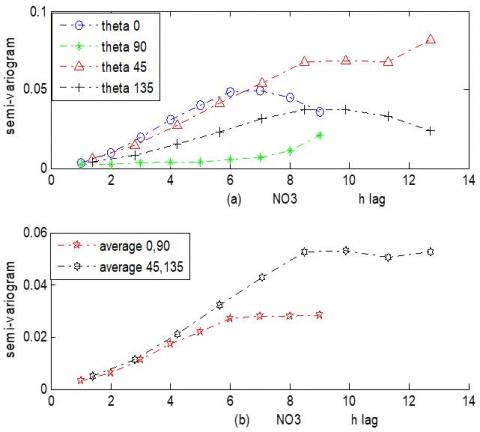
We use these data to illustrate the effect of pollution, and how and how to reduce this pollution. Figure 1 below describes the results of the variogram function for soil data NO3, where Figure 1(a) is for all theta of the compass, East-west (theta 0), North-south (theta 90), Northeast (theta 45), Northwest (theta135), while Figure 1(b) gives the average of the semi-variogram for two thetas based on the lag(h) according to Eq. (1).
Figure 1. Results of the semi-variogram of (NO3) data
Table 1 shows the results of the semi-variogram for all theta (G1 of that 0, G2 for that 90, G3 for that 45, and G4 for theta of 135), according to Eq. (1), while G5 for average (0.90), and G6 for average (45,135).
Table 1. Results of the semi-variogram with their average for (NO3) data
|
G1 |
0.0357 |
0.0448 |
0.0494 |
0.0484 |
0.0400 |
0.0309 |
0.0196 |
0.0097 |
0.0035 |
|
G2 |
0.0212 |
0.0112 |
0.0065 |
0.0054 |
0.0042 |
0.0040 |
0.0029 |
0.0023 |
0.0025 |
|
G3 |
0.0818 |
0.0681 |
0.0685 |
0.0677 |
0.0541 |
0.0414 |
0.0272 |
0.0145 |
0.0063 |
|
G4 |
0.0234 |
0.0330 |
0.0375 |
0.0375 |
0.0315 |
0.0232 |
0.0154 |
0.0083 |
0.0037 |
|
G5 |
0.0284 |
0.0280 |
0.0279 |
0.0269 |
0.0221 |
0.0174 |
0.0112 |
0.0060 |
0.0030 |
|
G6 |
0.0526 |
0.0506 |
0.0530 |
0.0526 |
0.0428 |
0.0323 |
0.0213 |
0.0114 |
0.0050 |
Table 2 illustrates the properties of the semi-variogram of (NO3) data for=0°,90°,45°,135°, and the average of the semi-variogram for two theta (0°, 90°), and (45°, 135°). Where (co =0.002989), (c+co=0.02843), and a=8), the curve of theta (0°, 90°) is nearest to the covariance model (spherical model):
$\gamma(h)=\left(\begin{array}{cll}c_o+c & , & h>a \\ c_o+c\left[\frac{3}{2}\left(\frac{h}{a}\right)-\frac{1}{2}\left(\frac{h}{a}\right)^3\right] & , & h<a \\ c_o & , & h=a\end{array}\right)$
where, a is the range, co is the Nugget effect and co+c is the sill [20].
Table 2. Properties of the semi-variogram for (NO3) data
|
Prop. θ |
Nugget Effect |
Sill |
Range |
Mean |
Median |
Median |
|
0° |
0.003495 |
0.04935 |
8 |
0.03131 |
0.03566 |
0.03566 |
|
90° |
0.002282 |
0.0212 |
8 |
0.006694 |
0.004195 |
0.004195 |
|
45° |
0.006284 |
0.0818 |
11.31 |
0.04773 |
0.05411 |
0.05411 |
|
135° |
0.003687 |
0.03756 |
11.31 |
0.02373 |
0.02341 |
0.02341 |
|
(0°, 90°) |
0.002989 |
0.02843 |
8 |
0.019 |
0.02209 |
0.02209 |
|
(45°, 135°) |
0.004986 |
0.053 |
11.31 |
0.03573 |
0.04282 |
0.04282 |
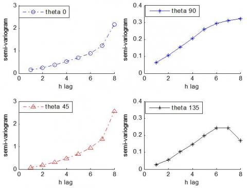
Figure 2 shows the results of the semi-variogram after taking the logarithm of the original data of (NO3). The curves of the semi-variogram describe the function of theta of the (0o, 90o, 45o, and 135o).
Figure 2. Results of the semi-variogram function after taking the logarithm of (NO3) data
Table 3 illustrates the properties of the semi-variogram after taking the logarithm of origin data of NO3. Properties of the semi-variogram include (nugget effect, sill, range, mean, median, and mode) with a theta of compass according the properties of semi-variogram.
Table 3. Properties of the semi-variogram for log (NO3)
|
Mode |
Median |
Mean |
Range |
Sill |
Nugget Effect |
Prop. |
|
Theta |
||||||
|
0.1542 |
0.6046 |
0.7842 |
7 |
2.166 |
0.1542 |
θ=0° |
|
0.0648 |
0.2317 |
0.2143 |
7 |
0.3214 |
0.0648 |
θ=90° |
|
0.08217 |
0.5762 |
0.82 |
7 |
2.562 |
0.08217 |
θ=45° |
|
0.02687 |
0.158 |
0.1483 |
7 |
0.2432 |
0.02687 |
θ=135° |
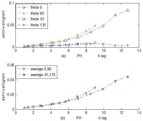
Figure 3 shows the curves of the semi-variogram function of soil data (PH), Figure 3(a) describes the results for all theta of the compass, and Figure 3(b) illustrates the semi-average of the semi-variogram for two thetas based on the lag (h).
Figure 3. Results of the semi-variogram function of (PH) data
Table 4 shows the properties of the average variogram function of (PH) data for two thetas of compass based on lag (h).
Table 4. Properties of the average semi-variogram function of (PH) data
|
Prop. |
Nugget Effect |
Sill |
Range |
Mean |
Median |
Mode |
|
Theta |
||||||
|
θ=0°, 90° |
0.001787 |
0.02963 |
8 |
0.01175 |
0.008449 |
0.001787 |
|
θ=45°, 135° |
0.002715 |
0.04429 |
11.31 |
0.01904 |
0.01474 |
0.002715 |
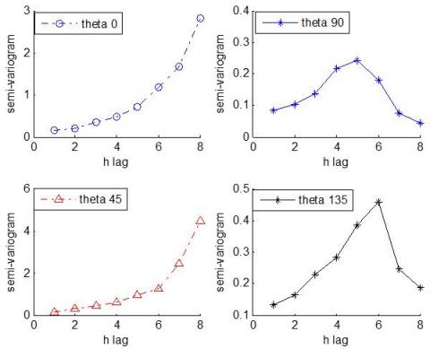
Figure 4 illustrates the results of the semi-variogram function of log (PH) data with the x-axis represented the lag (h), and the y-axis is a semi-variogram function in thetas (0o,90o,45o, and 135o).
Figure 4. Results of semi-variogram function of log (PH) in all thetas
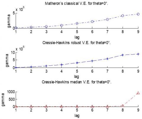
Figure 5. Three methods of robust variogram function
Figure 5 illustrates three methods of variogram (Matheron's classical, Cressie Hawkins robust, and Cressie Hawkins median) for theta 0 of soil data (NO3). According to the Eqs. (13)-(15).
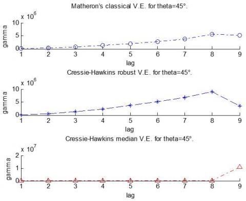
Figure 6. Three methods of variogram (Matheron's classical, Cressie Hawkins robust, and Cressie Hawkins median) for theta 45 of soil data (NO3)
Figure 6 illustrates three methods of variogram (Matheron's classical, Cressie Hawkins robust, and Cressie Hawkins median) for theta 45 of soil data (NO3).
Because of the small effect of extreme values on the estimates, it is clear from this effect that pollution may be large by properly knowing the weight restrictions for the level of pollution, and reducing the level of pollution depends practically and for a long period whenever some estimates lose their stability or constancy. The characteristics of robustness methods are studied using a prediction study and the results indicate several factors that affect the efficiency of the analyzed methods. In particular, the methods depend on: whether the data set is multivariate normal or not; the Dimension of the data set; Type of outliers. The proportion of outliers in the data set; and the degree of contamination of outliers (dimension). The study prompted the authors to recommend the use of “a combination of multivariate methods” on the data set to detect potential outliers. We fully adopt this recommendation and consider that the combination of methods should depend, but also on other factors such as the dimension and size of the data structure. Masking of one outlier by another outlier occurs if the second outlier can be considered an outlier in itself only, but not in the presence of the first outlier. Thus, because of this masking, a set of outlying observations skews the mean and covariance estimates toward it. the results showed the outliers Matheron median of variogram predict as corresponding to the theoretical model. For data without outliers, Matheson's and Haslett's robust estimators had better performance than Cressie Hawkins's robust soil data comparison with the empirical variogram. Soil data showed the spatial dependence of the variation at different scales.
The author of the research extends his thanks to the College of Education for Pure Sciences at the University of Mosul, which helped describe improving the quality of this research. He also thanks the contributors for evaluating and publishing the research.
[1] Matheron, G. (1973). The intrinsic random functions and their applications. Advances in Applied Probability, 5(3): 439-468. https://doi.org/10.2307/1425829
[2] Rendu, J.M.M. (1979). Normal and lognormal estimation. Mathematical Geology, 11: 407-422. https://doi.org/10.1007/BF01029297
[3] Dowd, P.A. (1982). Lognormal kriging—The general case. Mathematical Geology 14: 475-499. https://doi.org/10.1007/BF01077535
[4] Saito, H., McKenna, S.A., Zimmerman, D.A., Coburn, T.C. (2005). Geostatistical interpolation of object counts collected from multiple strip transects: Ordinary kriging versus finite domain kriging. Stochastic Environmental Research and Risk Assessment, 19: 71-85. https://doi.org/10.1007/s00477-004-0207-3
[5] Rousseeuw, P.J., Hubert, M. (2011). Robust statistics for outlier detection. Wiley Interdisciplinary Reviews: Data Mining and Knowledge Discovery, 1(1): 73-79. https://doi.org/10.1002/widm.2
[6] Kalina, J. (2018). A robust pre-processing of BeadChip microarray images. Biocybernetics and Biomedical Engineering, 38(3): 556-563. https://doi.org/10.1016/j.bbe.2018.04.005
[7] Víšek, J.Á. (2010). Robust error-term-scale estimate. In Nonparametrics and Robustness in Modern Statistical Inference and Time Series Analysis: A Festschrift in honor of Professor Jana Jurečková, pp. 254-268. https://doi.org/10.1214/10-IMSCOLL725
[8] Wang, X., Jiang, Y., Huang, M., Zhang, H. (2013). Robust variable selection with exponential squared loss. Journal of the American Statistical Association, 108(502): 632-643. https://doi.org/10.1080/01621459.2013.766613
[9] Wang, N., Wang, Y. G., Hu, S., Hu, Z. H., Xu, J., Tang, H., Jin, G. (2018). Robust regression with data-dependent regularization parameters and autoregressive temporal correlations. Environmental Modeling & Assessment, 23: 779-786. https://doi.org/10.1007/s10666-018-9605-7
[10] Kalina, J., Neoral, A. (2019). A robustified metalearning procedure for regression estimators. In Conference Proceedings, The 13th International Days of Statistics and Economics MSED, pp. 617-726.
[11] Jiang, Y., Wang, Y. G., Fu, L., Wang, X. (2019). Robust estimation using modified Huber’s functions with new tails. Technometrics, 61(1): 111-122. https://doi.org/10.1080/00401706.2018.1470037
[12] De Oliveira, C.C., Tiglea, P., Olivieri, J.C., Carvalho, M., Buzzo, M.L., Sakuma, A.M., Maria Cristina DURAN, Miriam Solange Fernandes CARUSO, Granato, D. (2014). Comparison of different statistical approaches used to evaluate the performance of participants in a proficiency testing program. Revista do Instituto Adolfo Lutz, 73(1): 26-31.
[13] Erdin, R., Frei, C., Künsch, H.R. (2012). Data transformation and uncertainty in geostatistical combination of radar and rain gauges. Journal of Hydrometeorology, 13(4): 1332-1346. https://doi.org/10.1175/JHM-D-11-096.1
[14] Cressie, N. (1993). Geostatistics: A tool for environmental modelers. In Environmental Modeling with GIS.
[15] Webster, R., Oliver, M.A. (2007). Geostatistics for Environmental Scientists. John Wiley & Sons.
[16] Lichtenstern, A. (2013). Kriging methods in spatial statistics. Bachelor’s Thesis, Technische Universität München (TUM), Munich, Germany.
[17] Cressie, N., Hawkins, D.M. (1980). Robust estimation of the variogram: I. Journal of the international Association for Mathematical Geology, 12: 115-125. https://doi.org/10.1007/BF01035243
[18] Kirchner, J.W., Knapp, J.L. (2020). Calculation scripts for ensemble hydrograph separation. Hydrology and Earth System Sciences, 24(11): 5539-5558. https://doi.org/10.5194/hess-2020-330
[19] Midi, H., Muhammad, S. (2018). Robust estimation for fixed and random effects panel data models with different centering methods. Journal of Engineering and Applied Sciences, 13(17): 7156-7161. https://doi.org/10.3923/jeasci.2018.7156.7161
[20] Somayasa, W., Sutiari, D.K., Sutisna, W. (2021). Optimal prediction in isotropic spatial process under spherical type variogram model with application to corn plant data. In Journal of Physics: Conference Series, 1940(1): 012003. https://doi.org/10.1088/1742-6596/1940/1/012003