Amenah Nazar Jabbar![]() | Hakan Koyuncu*
| Hakan Koyuncu*![]()
© 2023 IIETA. This article is published by IIETA and is licensed under the CC BY 4.0 license (http://creativecommons.org/licenses/by/4.0/).
OPEN ACCESS
Plant disease outbreaks have a profound impact on the agricultural sector, leading to substantial economic implications, compromised crop yields and quality, and potential food scarcity. Consequently, the development of effective disease prevention and management strategies is crucial. This study introduces a novel methodology employing deep learning for the identification and diagnosis of plant diseases, with a focus on mitigating the associated detrimental effects. In this investigation, Convolutional Neural Networks (CNNs) were utilized to devise a disease identification method applicable to three types of plant leaves - peppers (two classes), potato (three classes), and tomato (nine classes). Preprocessing techniques, including image resizing and data augmentation, were adopted to facilitate the analysis. Additionally, three distinct feature extraction methods - Haralick feature, Histogram of Gradient (HOG), and Local Binary Patterns (LBP) - were implemented. The Grey Wolf Optimization (GWO) technique was employed as a feature selection strategy to identify the most advantageous features. This approach diverges from traditional methodologies that solely rely on CNNs for feature extraction, instead extracting features from the dataset through multiple extractors and passing them to the GWO for selection, followed by CNN classification. The proposed method demonstrated high efficiency, with classification accuracies reaching up to 99.8% for pepper, 99.9% for potato, and 95.7% for tomato. This study thus provides a progressive shift in plant disease detection, offering promising potential for improving agricultural health management. In conclusion, the integration of deep learning and the Grey Wolf Optimization technique presents a compelling approach for plant disease detection, demonstrating high accuracy and efficiency. This research contributes a significant advancement in the field of agricultural health and disease management.
GWO, CNN, LBP, HOG, plant diseases
Plants are a crucial energy source and an excellent solution to address global warming. However, they are susceptible to numerous diseases that can have severe adverse effects on the environment, society, and the economy, potentially causing a significant decline in crop yield and quality [1]. Agriculture provides livelihood for 50% of the world's population, with the waste from harvesting serving as a source of income and sustenance, including products such as wax, oil, and jute [2].
In plant systems, emerging, re-emerging, and endemic diseases cause significant damage and can result in financial loss. Moreover, plant diseases indirectly and directly propagate infectious diseases that threaten humans and the environment. The spread of these diseases not only harms the plant's functionality but also the economy by limiting the amount of crop that can be grown [3]. Plant diseases can affect various plant components, including fruits, stems, and leaves. The most common bacterial, fungal, and viral diseases in plants are Alternaria, Anthracnose, bacterial spot, canker, and others.
Environmental changes often cause viral illnesses, bacterial diseases are brought on by germs in plant leaves, and fungal illnesses are caused by leaf fungi [4]. Plant diseases frequently threaten the output and quality of global agricultural products, contributing to a significant amount of production costs. It is estimated that plant disease losses have reduced global food output by at least 10% [5].
Awareness of the detrimental effects of extensive chemical pesticide usage on the environment and health is increasing. Consumers now prefer organically grown food. Additionally, regulatory bodies like the European Union (EU) are tightening restrictions on the use of chemicals in agricultural goods imported into their markets. These developments underline the need for early and accurate detection of pests and diseases, highlighting the importance of reducing pesticide use in agriculture [6].
Plant disease prevention and control have been the subject of intense discussion as plants, exposed to the outside environment, are extremely susceptible to infections. Accurate and rapid disease identification is crucial in effectively combating plant diseases, as it often leads to effective protective measures [7]. Plant diseases commonly reduce yields, quality, and economic growth. Therefore, professional observation with the naked eye is labor-intensive, and automation for identifying leaf diseases is a significant area of research [8].
It has now become necessary to identify and diagnose plant diseases using information technology. Techniques such as automated plant disease identification and categorization must be developed by employing leaf image processing methods. These techniques will serve as a beneficial strategy for farmers, providing early warnings before the disease spreads widely [9].
1.1 Type of plant diseases
Crop leaves are particularly susceptible to disease. Pathogens, including viruses, bacteria, fungi, and deficiencies, severely affect crops. Consequently, pathogens are categorized into two types: autotrophs, which feed on living tissue, and saprophytes, which feed on dead tissue. The symptoms of these diseases, which hinder crop development and growth, are clearly visible. The first sign of illness in plants is often discolored leaves [10].
In addition, the texture and shape of the leaves can be used to identify several diseases. Therefore, processing images of the leaves can help identify diseases such as mildew, rust, and powdery mildew [11]. There are three types of viruses and contagious plant diseases, as shown in Figure 1.
Figure 1. Types of viruses and contagious plant diseases
1.2 Fungal diseases
Fungi cause the majority of vegetable diseases. Fungal infections stress plants and destroy their cells. These infections can originate from various sources, including contaminated seeds, unsuitable soil, agricultural waste, neighboring crops, and weeds. Their focal points are the organic apertures, like the stomata in plants. Fungal growth can also occur inside plants when artificial wounds are created by pruning, harvesting, flooding, insects, or other diseases [12].
1.3 Bacteria diseases
Many parts of plants are susceptible to bacterial infections. Bacteria can affect plants internally without showing any outward symptoms. Cankers, leaf spots, overgrowth, scabs, and wilts are among the signs that a plant is infected by bacteria. An infected plant can serve as a source of infection for other nearby plants, rapidly spreading the disease [13].
1.4 Viral diseases
Viral infections affecting plant leaves are the most challenging to identify. Most viruses are latent, meaning they cannot be detected until they reach a certain level. It is common to confuse viral infections with nutritional deficiencies and pesticide damage. Carriers such as aphids, leafhoppers, whiteflies, cucumber beetles, and other insects can easily transmit viruses [14].
1.5 Related works
Given the importance of plants in providing food, reducing global warming, and acknowledging the serious negative environmental impact of plant diseases, it's necessary to find quick and accurate solutions for plant disease detection.
This section presents a discussion of the proposed deep learning techniques which is represented by the CNN for this paper and the optimization algorithm (GWO) in addition to the mathematical formula used to reduce and improve the extracted features.
2.1 Data collection
In this paper the dataset obtained from The Plant Village dataset is a large collection of images of plant diseases was used. It was compiled by researchers at Penn State University. The dataset includes over 50,000 images of over 38 different species of plants, with diseases ranging from bacterial spots to rust to powdery mildew.
The next step will be data preprocessing, it will go through two steps: data resize and data augmentation. Figure 2 shows the preprocessing path.
Figure 2. Images preprocessing path
2.2 Features extraction
Feature extraction is a process in which specific characteristics or features of an image are extracted and made available for further processing [22]. In computer vision, we employ a variety of classifiers, each with their own set of properties and attributes [23]. Haralick, the Histogram of Oriented Gradients (HOG), and Local Binary Patterns (LBP) in this paper were used to extract the features.
2.2.1 Local binary patterns (LBP)
A texture descriptor used describes the texture of an image. It compares the values of nearby pixels within each zone after segmenting a picture into smaller sections. The center pixel acts as a threshold for the neighboring pixel in the LBP, which uses a 3x3-bit block size. The center pixel's LBP code is created by converting the computed threshold value to a decimal value [24]. See Figure 3.
Figure 3. LBP operation
In this system, LBP was used to extract the features of the images dataset, 59 features were extracted by this descriptor.
2.2.2 Histogram of oriented gradients (HOG)
This feature descriptor is used in computer vision and image processing to describe the structure and form of an item in an image. It computes the distribution of intensity gradients inside each cell by segmenting the picture into tiny cells. The method counts the occurrences of a gradient orientation in a certain area of a picture [25]. In this system, HOG was used to extract the features of the images dataset, 36 features were extracted by this descriptor.
2.2.3 Haralick texture
The texture of an image may be described using the Haralick. Gray level co-occurrence matrix (GLCM) computations based on the characteristics of the Haralick texture are widely used to represent picture texture since they are simple to implement and result in a set of understandable texture descriptors [26]. This system, GLCM was used to extract the features of the images dataset, 14 features were extracted by this descriptor.
2.3 Gray wolf optimization (GWO)
The GWO algorithm functions by modeling a pack of grey wolves hunting for prey. The alpha wolf, beta wolf, and delta wolf are the algorithm's three major operators. The pack's leader and search coordinator are known as the alpha wolf. The second in leadership, the beta wolf, is in charge of searching the area. The third-in-command, known as the delta wolf, is in charge of utilizing the most effective solutions so far [27, 28].
2.4 Mathematical model for GWO
It chooses the fittest solution as the alpha (α) while constructing GWO to mathematically reproduce the wolf pack. Hence, the second- and third-best solutions are designated as beta (β) and delta (δ), respectively. The GWO algorithm hunts for the remaining viable solutions, which are all viewed as being omega (ω). These three wolves are followed by the remaining wolves [29].
2.4.1 Encircling
Grey wolves hunt by encircling their victim. The encircling behavior is quantitatively described by the following equations [30]:
$\vec{D}=\left|\vec{C} \cdot \overrightarrow{x_p}(t)-\vec{x}(t)\right|$ (1)
$\vec{x}(t+1)=\vec{x}_p(t)-\vec{A} \cdot \vec{D}$ (2)
where, $t$ shows the most recent iteration, $\vec{A}$ and $\vec{D}$ are vectors of coefficients, $\overrightarrow{x_p}$ is the prey's location vector, and $\vec{x}$ shows a grey wolf's location vector. This is how the vectors $\vec{A}$ and $\vec{C}$ are calculated:
$\vec{A}=2 \vec{a} \cdot \overrightarrow{r_1}-\vec{a}$ (3)
$\vec{C}=2 \cdot \overrightarrow{r_2}$ (4)
where, $\overrightarrow{r_1}$ and $\overrightarrow{r_2}$ are random vectors in the range $[0,1]$ and components of $\vec{a}$ are linearly decreased from 2 to 0 during the duration of repetitions.
2.4.2 Hunting
While beta and delta have a better grasp of the likely location of prey, alpha is thought to be the optimum solution. The remaining wolves (including omegas (ω)) must update their places depending on the position of the best answer, and the three best solutions found thus far are maintained. The following equations are provided in this regard [30]:
$\begin{gathered}\vec{D}_a=\left|\vec{C}_1 \cdot \vec{x}_a-\vec{x}\right|, \vec{D}_\beta=\left|\vec{C}_2 \cdot \vec{x}_\beta-\vec{x}\right|, \vec{D}_\delta= \left|\vec{C}_3 \cdot \vec{x}_\delta-\vec{x}\right|\end{gathered}$ (5)
$\begin{aligned} & \vec{x}_1=\vec{x}_\alpha-\vec{A}_1 \cdot\left(\vec{D}_\alpha\right), \vec{x}_2=\vec{x}_\beta-\vec{A}_2 \cdot\left(\vec{D}_\beta\right), \vec{x}_3=\vec{x}_\delta-\vec{A}_3 \cdot\left(\vec{D}_\delta\right)\end{aligned}$ (6)
$\vec{x}(t+1)=\frac{\vec{x}_1+\vec{x}_2+\vec{x}_3}{3}$ (7)
These equations allow a search agent to modify its position in an n-dimensional search space to account for alpha, beta, and delta. The alpha, beta, and delta wolves predict where the prey is while the remaining wolves update their locations at random around the prey [31].
2.4.3 Attacking
As the prey stops moving, the grey wolves finish the hunt by attacking it. In order to mathematically imitate approaching the prey, the value of $\vec{a}$ is decreased. It is worth mentioning that decreases $\vec{A}$ fluctuation range. In other words, $\vec{A}$ is a random value in the range $[-2 \alpha, 2 \alpha]$, with a decreasing from 2 to 0 during the period of repetitions. When random values of $\vec{A}$ are in the range $[-1,1]$, the future position of a search agent can be anywhere between its present position and the position of the prey. Figure 4 show that $|A|<1$ forces the wolves to attack towards the prey [32].
Figure 4. Attacking prey
2.4.4 Searching
Grey wolves usually search using the alpha $(\alpha)$, beta $(\beta)$, and delta (o) positions. They divide to look for prey and then converge to attack prey $\vec{A}$ employs random values larger than 1 or less than -1 to force the search agent to diverge from the prey in order to mathematically describe divergence. This promotes exploration and allows the GWO algorithm to do extensive exploration illustrates that $|A|>1$ causes the grey wolves to deviate from the prey in the hopes of finding a fitter prey [30, 32].
The objective of GWO is to identify the subset of characteristics that improves the model's performance. By combining the results of Local binary pattern (LBP), Histogram of oriented gradients (HOG), and Haralick texture features, the next step will be applying GWO algorithm steps to these features to select the most efficient features. These are the steps of the algorithm that was followed to build the optimization algorithm in this research.
Step 1. Load the LBP, HOG, and Haralick features
Step 2. Concatenate the features
X=[LBP HOG Haralick];
Step 3. Define the search space.
d=size(X, 2);
searchSpace=zeros(d, d);
Step 4. Define the objective function.
objFcn=@(subset) modelPerformance(X(:, subset), y);
Step 5. Define the stopping criteria.
maxIter=100; //Max Iteration
Step 6. Initialize the positions of the alpha, beta, and delta wolves.
alpha=randi(d);
beta=randi(d);
delta=randi(d);
Step 7. Initialize the best solution.
bestSol=zeros(d, 1);
bestVal=-inf;
Step 8. Run the GWO algorithm.
For iter: $\leftarrow$ 1 to maxIter
//Calculate the objective function value for each wolf
alphaVal=objFcn(alpha);
betaVal=objFcn(beta);
deltaVal=objFcn(delta);
//Update the positions of the wolves
alpha=updatePosition (alpha, alphaVal, betaVal, deltaVal, searchSpace);
beta=updatePosition (beta, alphaVal, betaVal, deltaVal, searchSpace);
delta=updatePosition (delta, alphaVal, betaVal, deltaVal, searchSpace);
//Update the best solution
if alphaVal>bestVal
bestSol=alpha;
bestVal=alphaVal;
end
if betaVal>bestVal
bestSol=beta;
bestVal=betaVal;
end
if deltaVal>bestVal
bestSol=delta;
bestVal=deltaVal;
end
GWOFeatures$\leftarrow$bestVal
end For
Return GWOFeatures
3.1 Convolution neural networks
Convolutional neural network (CNN) is a multilayer perceptron (MLP) network. The human brain serves as an inspiration for CNN's computers. A CNN needless pre-processing and feature extraction work since it combines the feature extraction and classification operations [33]. The convolutional layer, the pooling layer, and the output layer make form a fundamental convolutional neural network. Sometimes a pooling layer is not necessary with three convolutional layers in Figure 5. The input layer, many hidden layers (repetition of convolutional, normalizing, and pooling), a fully connected layer, and an output layer make up the system [34].
Figure 5. Typical convolutional neural network architecture
Although CNN does not need pre-processing and feature extraction, in this paper we used three feature descriptors to extract features and passed them to the GWO algorithm to improve and reduce these features. Then we used a two-dimensional neural network to build the classification model.
4.1 Proposed model
The dataset contains three types of plants: pepper (two types: healthy and bacterial spot), potatoes (three types: healthy, early blight, and late blight), and tomatoes (nine types: healthy, target spot, tomato yellow leaf curl virus, bacterial spot, early blight, late blight, leaf mold, Septoria leaf spot, and spider mites, two-spotted spider mite). The working principle of the proposed model will be as follows. After pre-processing the data, it will be divided into 80% training, 20% testing and three methods-local binary patterns (LBP), histogram of oriented gradients (HOG), and Haralick-are used to extract features from the data. Then, it is passed to the gray wolf algorithm to choose the best features, and finally, the convolutional neural network (CNN) deep learning method is then trained to identify the correct disease diagnosis for each plant. Figure 6 shows the proposed model flows.
Figure 6. Proposed system block diagram
4.2 Results of implementation system
This section is divided into four phases: Data preprocessing, Feature extraction, feature selection, and CNN algorithms training.
Data preprocessing is a step-in data analysis that involves image resize, and data augmentation.
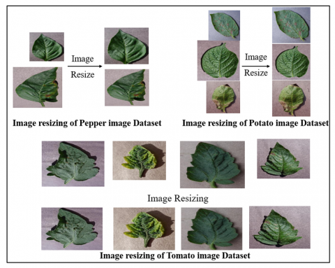
5.1 Image resize
All images in the dataset will be resized to 256 pixels in width and 256 pixels in height during the loading process. Figure 7 showed resized images.
Figure 7. Dataset samples for images resizing
5.2 Data augmentation
To increase the amount of data each class in dataset was augmented using three transformation functions X-reflection, Y-reflection, and Rotation. Table 1 shows the augmentation results for each class. Table showed the augmented data.
Table 1. Augmentation results
|
Class |
Original Size |
Augmented Size |
|
Pepper |
2455 |
7,365 |
|
Potato |
2152 |
6,456 |
|
Tomato |
16,013 |
48,039 |
|
Total |
20,620 |
61,851 |
Table 2. Features extraction
|
Method |
Number of Features |
|
LBP |
59 |
|
HOG |
36 |
|
Haralick |
14 |
|
Total |
109 |
Three techniques-local binary pattern (LBP), histogram of oriented gradients (HOG), and Haralick texture features-were used to extract the features from the dataset images. The number of characteristics that were retrieved from each class is shown in Table 2.
For three types of plant leaves, pepper, potato, and tomato, and for the two classes, three classes, and nine classes, results were obtained by using different population samples (125, 150, 175 and 200), 1900 instants for the pepper ,2200 instants for the potato and 12000 instants for the tomato, 0.3 threshold, 50 iterations, and a 70:30% training-to-testing ratio for the three plant types: pepper, potato, and tomato. The number of features that were chosen for five rounds is shown in Table 3.
Table 3. Feature selection results for different population in pepper, potato and tomato
|
Pepper |
|||||
|
no. of features |
|||||
|
Pop size |
round 1 |
round 2 |
round 3 |
round 4 |
round 5 |
|
150 |
48 |
29 |
23 |
35 |
25 |
|
175 |
37 |
30 |
29 |
40 |
21 |
|
200 |
35 |
87 |
21 |
47 |
35 |
|
Potato |
|||||
|
no. of features |
|||||
|
Pop size |
round 1 |
round 2 |
round 3 |
round 4 |
round 5 |
|
150 |
21 |
25 |
37 |
25 |
38 |
|
175 |
53 |
22 |
29 |
33 |
36 |
|
200 |
26 |
34 |
22 |
23 |
37 |
|
Tomato |
|||||
|
|
no. of features |
||||
|
Pop size |
round 1 |
round 2 |
round 3 |
round 4 |
round 5 |
|
150 |
58 |
74 |
21 |
47 |
22 |
|
175 |
21 |
27 |
30 |
23 |
22 |
|
200 |
24 |
21 |
47 |
21 |
22 |
Plant disease classification was taught to the Convolution Neural Network (CNN) in two types of pepper, three types of potato, and nine types of tomato, and those were classified at several epochs (500, 600, 700, 800, 900, and 1000). Tables 4, 5 and 6 show the details of CNN-model results with training accuracy for the three plants leaf’s types.
For the pepper plants, as shown in the above table, when taking into account the minimum implementation time, the best accuracy results (99.80%) we obtained were in this case 600 epoch, 9000 max-iteration in 5min, 16sec execution time. Knowing that CNN, in this case, classified 2 types of leaves, one is healthy and the other infected disease.
Table 4. CNN results in pepper
|
Epoch |
Max Iteration |
Iteration per Epoch |
Elapsed Time |
Accuracy |
|
500 |
7500 |
15 |
4min, 27sec |
99.70% |
|
600 |
9000 |
15 |
5min, 16sec |
99.80% |
|
700 |
10500 |
15 |
6min, 1sec |
99.80% |
|
800 |
12000 |
15 |
7min, 3sec |
98.60% |
|
900 |
13500 |
15 |
7min, 32sec |
96.70% |
|
1000 |
15000 |
15 |
8min, 27sec |
97.40% |
Table 5. CNN results in potato
|
Epoch |
Max Iteration |
Iteration per Epoch |
Elapsed Time |
Accuracy |
|
500 |
7500 |
15 |
4min, 30sec |
99.80% |
|
600 |
9000 |
15 |
5min, 13sec |
99.90% |
|
700 |
10500 |
15 |
5min, 58sec |
99.90% |
|
800 |
12000 |
15 |
6min, 21sec |
99.80% |
|
900 |
13500 |
15 |
6min, 34sec |
99.80% |
|
1000 |
15000 |
15 |
8min, 29sec |
99.90% |
Table 6. CNN results in tomato
|
Epoch |
Max Iteration |
Iteration per Epoch |
Elapsed Time |
Accuracy |
|
500 |
7500 |
15 |
3min, 43sec |
88.60% |
|
600 |
9000 |
15 |
5min, 1sec |
89.40% |
|
700 |
10500 |
15 |
5min, 31sec |
94.60% |
|
800 |
12000 |
15 |
6min, 39sec |
89.60% |
|
900 |
13500 |
15 |
7min, 34sec |
92.90% |
|
1000 |
15000 |
15 |
8min,57sec |
95.70% |
For the potato plants, as shown in the above table, when taking into account the minimum implementation time, the best accuracy results (99.90%) we obtained were in this case 600 epochs, 9000 max-iteration in 5min, 13sec execution time. Knowing that CNN, in this case, classified 3 types of leaves, one of which is healthy and the rest infected with 2 different types of diseases. Table 5.
For tomato plants, as shown in the table above, when considering the minimum execution time, the best accuracy results (95.70%) we obtained in this case were 1000 epochs, 15000 max-iteration in 58 min, 57 sec execution time. Knowing that CNN, in this case, classified 9 types of leaves, one of which is healthy and the rest infected with 8 different types of diseases. Table 6.
According to CNN model the training reached a maximum of 7500 iterations by 15 iterations per epoch with a maximum epoch of 500 in the first case, and a maximum of 12000 iterations by 15 iterations per epoch with a maximum epoch of 800 in the second case. Figures 8, 9 show the graphical results for the two cases of the CNN model training in pepper plants indicating that total accuracy has reached the highest level and losses have reached their lowest level.
In potato plant and according to CNN model the training reached a maximum of 7500 iterations by 15 iterations per epoch with a maximum epochs of 500 in the first case, and a maximum of 12000 iterations by 15 iterations per epoch with a maximum epochs of 800 in the second case Figures 10, 11 show the graphical results for the two cases of the CNN model training in potato plants indicating that total accuracy has reached the highest level and losses have reached their lowest level. In tomato plant and according to CNN model the training reached a maximum of 7500 iterations by 15 iterations per epoch with a maximum epochs of 500 in the first case, and a maximum of 12000 iterations by 15 iterations per epoch with a maximum epochs of 800 in the second case Figures 12, 13 shows the graphical results for the two cases of the CNN model training in tomato plants indicating that total accuracy has reached the highest level and losses have reached their lowest level.
Figure 8. Accuracy and loss progress in pepper plants at 500 epochs using CNN
Figure 9. Accuracy and loss progress in pepper plants at 800 epochs using CNN
Figure 10. Accuracy and loss progress in potato plants at 500 epochs using CNN
Figure 11. Accuracy and loss progress in potato plants at 800 epochs using CNN
Figure 12. Accuracy and loss progress in tomato plants at 500 epochs using CNN
Figure 13. Accuracy and loss progress in tomato plants at 800 epochs using CNN
Based on the results obtained from the proposed system, the accuracy obtained by extracting features from LBP, HOG and Haralick after competing and optimizing by GWO and classifying by CNN achieved better results compared to the results of the traditional CNN, as shown in the Table 7 below.
Table 7. The accuracy in some systems compared with the propose system
|
Model |
Techniques |
Accuracy% |
|
Harakannanavar et al. [12] |
CNN |
99.6% |
|
Sullca et al. [15] |
CNN |
84% |
|
Anagnostis et al. [16] |
CNN |
98.7% |
|
Geetharamani and Pandian [18] |
CNN |
96.4% |
|
Zhang et al. [20] |
CNN |
94.2% |
|
Lu et al. [21] |
CNN |
95.4% |
|
Proposed system |
CNN-pepper |
99.8% |
|
CNN-Potato |
99.9% |
|
|
CNN-Tomato |
95.7% |
Plant diseases commonly reduce yields, quality, and economic growth. This case clearly demonstrates that professional observation with the unaided eye requires a lot of work, and as a result, automation to identify leaf diseases consumes a significant amount of research. This paper proposes the classification of plants using convolutional neural networks. Three types of plants were classified: pepper, potato, and tomato, where pepper was a binary class, potato was the three classes, and tomato was the nine classes. Three types of feature extractors were used, which are histogram of oriented gradients (HOG), local binary pattern (LBP) and Haralick texture features, and these features were passed on to the gray wolf optimization algorithm after it was done, which is an optimization algorithm that functions by modeling a pack of gray wolves hunting for prey. Classification by convolutional neural networks showed the best accuracy for pepper (99.8%), potato (99.9%), and tomato (95.7%).
[1] Sindhu, P., Indirani, G. (2020). IoT based wheat leaf disease classification using hybridization of optimized deep neural network and grey wolf optimization algorithm. Annals of the Romanian Society for Cell Biology, 35-53.
[2] Anjana., Keshav, K. (2018). Plant leaf disease classification and detection with CNN and optimization. International Journal of Research in Electronics and Computer Engineering (IJRECE), ISSN: 2393-9028.
[3] Nagaraju, M., Chawla, P. (2020). Systematic review of deep learning techniques in plant disease detection. International Journal of System Assurance Engineering and Management, 11: 547-560. https://doi.org/10.1007/s13198-020-00972-1
[4] Hemavathi, S., Hemachandran, V.K., Mothish, D., Ramprakash, M. (2020). Plant uses and disease identification using SVM technology. Ilkogretim Online, 19(3): 4626-4633.
[5] Prakash, R.M., Saraswathy, G.P., Ramalakshmi, G., Mangaleswari, K.H., Kaviya, T. (2017). Detection of leaf diseases and classification using digital image processing. In 2017 International Conference on Innovations in Information, Embedded and Communication Systems (ICIIECS). IEEE, pp. 1-4. https://doi.org/10.1109/ICIIECS.2017.8275915
[6] Ma, J., Du, K., Zheng, F., Zhang, L., Gong, Z., Sun, Z. (2018). A recognition method for cucumber diseases using leaf symptom images based on deep convolutional neural network. Computers and Electronics in Agriculture, 154: 18-24. https://doi.org/10.1016/j.compag.2018.08.048
[7] Ngugi, L.C., Abelwahab, M., Abo-Zahhad, M. (2021). Recent advances in image processing techniques for automated leaf pest and disease recognition-A review. Information Processing in Agriculture, 8(1): 27-51. https://doi.org/10.1016/j.inpa.2020.04.004
[8] Sun, G., Jia, X., Geng, T. (2018). Plant diseases recognition based on image processing technology. Journal of Electrical and Computer Engineering, 2018. https://doi.org/10.1155/2018/6070129
[9] Reeta Janet Jessy I, Mrs. N. Bindu M.E, Mr. N. Rajkumar M.E. (2016). Color co-occurrence and bit pattern feature based CBIR. International Journal of Scientific & Engineering Research, ISSN 2229-5518.
[10] Orchi, H., Sadik, M., Khaldoun, M. (2021). On using artificial intelligence and the internet of things for crop disease detection: A contemporary survey. Agriculture, 12(1): 9. https://doi.org/10.3390/agriculture12010009
[11] Yuvaraj, N., Karthikeyan, T., Praghash, K. (2021). An improved task allocation scheme in serverless computing using gray wolf Optimization (GWO) based reinforcement learning (RIL) approach. Wireless Personal Communications, 117(3): 2403-2421. https://doi.org/10.1007/s11277-020-07981-0
[12] Harakannanavar, S.S., Rudagi, J.M., Puranikmath, V.I., Siddiqua, A., Pramodhini, R. (2022). Plant leaf disease detection using computer vision and machine learning algorithms. Global Transitions Proceedings, 3(1): 305-310. https://doi.org/10.1016/j.gltp.2022.03.016
[13] Verma, S., Chug, A., Singh, A.P. (2018). Prediction models for identification and diagnosis of tomato plant diseases. In 2018 International Conference on Advances in Computing, Communications and Informatics (ICACCI). IEEE, pp. 1557-1563. https://doi.org/10.1109/ICACCI.2018.8554842
[14] Shah, J.P., Prajapati, H.B., Dabhi, V.K. (2016). A survey on detection and classification of rice plant diseases. In 2016 IEEE International Conference on Current Trends in Advanced Computing (ICCTAC), pp. 1-8. https://doi.org/10.1109/ICCTAC.2016.7567333
[15] Sullca, C., Molina, C., Rodríguez, C., Fernández, T. (2019). Diseases detection in blueberry leaves using computer vision and machine learning techniques. International Journal of Machine Learning and Computing, 9(5): 656-661. https://doi.org/10.18178/ijmlc.2019.9.5.854
[16] Anagnostis, A., Asiminari, G., Papageorgiou, E., Bochtis, D. (2020). A convolutional neural networks based method for anthracnose infected walnut tree leaves identification. Applied Sciences, 10(2): 469. https://doi.org/10.3390/app10020469
[17] Kaur, N., Devendran, V. (2020). Withdrawn: Novel plant leaf disease detection based on optimize segmentation and law mask feature extraction with SVM classifier. https://doi.org/10.1016/j.matpr.2020.10.901
[18] Geetharamani, G., Pandian, A. (2019). Identification of plant leaf diseases using a nine-layer deep convolutional neural network. Computers & Electrical Engineering, 76: 323-338. https://doi.org/10.1016/j.compeleceng.2019.04.011
[19] Balakrishna, K., Rao, M. (2019). Tomato plant leaves disease classification using KNN and PNN. International Journal of Computer Vision and Image Processing (IJCVIP), 9(1): 51-63. https://doi.org/10.4018/IJCVIP.2019010104
[20] Zhang, S., Huang, W., Zhang, C. (2019). Three-channel convolutional neural networks for vegetable leaf disease recognition. Cognitive Systems Research, 53: 31-41. https://doi.org/10.1016/j.cogsys.2018.04.006
[21] Lu, Y., Yi, S., Zeng, N., Liu, Y., Zhang, Y. (2017). Identification of rice diseases using deep convolutional neural networks. Neurocomputing, 267: 378-384. https://doi.org/10.1016/j.neucom.2017.06.023
[22] Kumar, T., Verma, K. (2010). A theory based on conversion of RGB image to gray image. International Journal of Computer Applications, 7(2): 7-10.
[23] Ahmed, A., Kurnaz, S., Hamdi, M., Khaleel, A., Jabbar, A., Seno, M. (2022). Detection of COVID-19 using classification of an x-ray image using a local binary pattern and k-nearest neighbors. International Symposium on Multidisciplinary Studies and Innovative Technologies (ISMSIT), Ankara, pp. 408-412. https://doi.org/10.1109/ISMSIT56059.2022.9932767
[24] Kaplan, K., Kaya, Y., Kuncan, M., Ertunç, H.M. (2020). Brain tumor classification using modified local binary patterns (LBP) feature extraction methods. Medical Hypotheses, 139: 109696. https://doi.org/10.1016/j.mehy.2020.109696
[25] Dalal, N., Triggs, B. (2005). Histograms of oriented gradients for human detection. In 2005 IEEE Computer Society Conference on Computer Vision and Pattern Recognition (CVPR'05), 1: 886-893. https://doi.org/10.1109/CVPR.2005.177
[26] Brynolfsson, P., Nilsson, D., Torheim, T., Asklund, T., Karlsson, C.T., Trygg, J., Nyholm, T., Garpebring, A. (2017). Haralick texture features from apparent diffusion coefficient (ADC) MRI images depend on imaging and pre-processing parameters. Scientific Reports, 7(1): 4041. https://doi.org/10.1038/s41598-017-04151-4
[27] Treisman, A.M., Gelade, G. (1980). A feature-integration theory of attention. Cognitive Psychology, 12(1): 97-136. https://doi.org/10.1016/0010-0285(80)90005-5
[28] Yadav, S., Verma, S. K., & Nagar, S. K. (2016). Optimized PID controller for magnetic levitation system. Ifac-PapersOnLine, 49(1), 778-782.
[29] Xie, Q., Guo, Z., Liu, D., Chen, Z., Shen, Z., Wang, X. (2021). Optimization of heliostat field distribution based on improved gray wolf optimization algorithm. Renewable Energy, 176: 447-458. https://doi.org/10.1016/j.renene.2021.05.058
[30] Mirjalili, S., Mirjalili, S.M., Lewis, A. (2014). Grey wolf optimizer. Advances in Engineering Software, 69: 46-61. https://doi.org/10.1016/j.advengsoft.2013.12.007
[31] Zareie, A., Sheikhahmadi, A., Jalili, M. (2020). Identification of influential users in social network using gray wolf optimization algorithm. Expert Systems with Applications, 142: 112971. https://doi.org/10.1016/j.eswa.2019.112971
[32] Sun, X., Hu, C., Lei, G., Guo, Y., Zhu, J. (2019). State feedback control for a PM hub motor based on gray wolf optimization algorithm. IEEE Transactions on Power Electronics, 35(1): 1136-1146. https://doi.org/10.1109/TPEL.2019.2923726
[33] Yamashita, R., Nishio, M., Do, R.K.G., Togashi, K. (2018). Convolutional neural networks: An overview and application in radiology. Insights into Imaging, 9: 611-629. https://doi.org/10.1007/s13244-018-0639-9
[34] Ahlawat, S., Choudhary, A., Nayyar, A., Singh, S., Yoon, B. (2020). Improved handwritten digit recognition using convolutional neural networks (CNN). Sensors, 20(12): 3344. https://doi.org/10.3390/s20123344