© 2018 IIETA. This article is published by IIETA and is licensed under the CC BY 4.0 license (http://creativecommons.org/licenses/by/4.0/).
OPEN ACCESS
This work investigates the performance of hybrid satellite terrestrial cooperative relaying communications network (HSTCN) over time-selective fading links arising due to the node mobility. Both satellite–to-destination (SD) and Satellite-to–relay (SR) links undergo the independent and identically distributed (i.i.d.) time-selective shadowed Rician fading, the terrestrial relay-to-destination links are assumed to be i.i.d. time-selective Nakagami-m faded. It evaluates the performance of such a network using multiple-input multiple-output (MIMO) space-time block-code (STBC) based selective decode-forward (S-DF) cooperation with imperfect CSI. An analytical approach is derived to evaluate the performance of the system in terms of per-frame average pairwise error probability (PEP) and asymptotic PEP floor. Further, a framework is developed for deriving the diversity order (DO). It demonstrates that full DO for cooperation protocol can be achieved when there is a knowledge of perfect CSI. A convex optimization (CO) framework is formulated for obtaining the optimal source-relay power allocation factors which significantly improve the end-to-end reliability of the system under power constraint scenarios. The results show the time selective nature of the links and imperfect CSI significantly degrades the system performance. Further, the impact of the satellite elevation angles at the terrestrial nodes is explicitly demonstrated through simulations. The error rate of the system is seen to reduce significantly with increasing satellite elevation angle at the relay when the SD link experiences frequent heavy shadowing and the RD links are relatively strong. However, for other scenarios when the RD links are relatively weak and SR links experience frequent heavy shadowing, significant performance improvement can be seen by increasing the satellite elevation angle at the destination user equipment. The analytical expressions show excellent agreement with the simulation results.
node mobility, selective decode-forward, space-time block code, hybrid satellite network, pairwise error probability
HSTCN are used in the context of mass broadcasting and navigation due to their ability to provide satellite coverage inside buildings and other shadowed areas. However, due to the rain, fog, poor angle of inclination, non-availability of line-of-sight (LOS), and low transmit power, the satellite coverage area is limited by the masking effect between the satellite and a terrestrial user. The masking effect becomes more severe in the case of low satellite elevation angles or when the user is indoor. The masking aberration also affects outdoor communication scenarios and its effect becomes more pronounced at lower satellite elevation angles. Further, mobility of the destination user-equipment (UE) and other cooperative UEs serving as relay nodes induces Doppler, which results in time-selective fading and the ensuing degradation of the end-to-end system performance (Varshney and Puri, 2017). Relay technology has thus become one of the core techniques in next-generation wireless communication systems. Therefore, HSTCN has been developed more recently to improve the performance as well as the coverage of the satellite networks (Ruan et al., 2017).
In (Yang and Hasna, 2015), HSTCN is proposed, to avoid the masking effect. However, the work therein considers the amplify-and-forward (AF) protocol, which introduces noise amplification at the relay nodes. In (Sreng et al., 2013), the authors investigated the symbol error rate (SER) performance of HSTCN. The closed form (CF) formulations for SER of quadrature phase shift keying (QPSK) and Quadrature amplitude modulation (QAM) signaling with maximum likelihood (ML) decoding over independent but not necessarily identically distributed shadowed rician fading channel are derived. These CF expressions are represented in terms of a finite sum of Lauricella hypergeometric functions. However, this work does not consider the impact of node mobility, elevation angles and imperfect CSI and on the PEP performance. In (Iqbal and Ahmed, 2011), the authors investigated the SER for a variable gain AF relaying network. Later, in (Bhatnagar and Arti, 2013), the authors investigated the performance of a fixed gain AF relaying system. Compared with variable-gain relaying, fixed-gain relaying appeals in practical applications for its ability to lower the implementation complexity since only statistic CSI is required. Further, several works such as (An et al., 2014; Sharma et al., 2016; Iqbal and Ahmed, 2015) have analyzed dual-hop HSTCN considering either AF or conventional decode-forward cooperative communication protocols at the relay node. However, in these works do not consider node mobility and imperfect CSI. In the authors investigated the node mobility and its impact on the per frame average PEP performance, especially employing the SDF cooperative protocol. However, in this work the authors do not consider MIMO and STBC and authors have not analyzed the diversity order and optimal power allocation. In (Halber and Chakravarty, 2018; Srikanth et al., 2018) the author has desribed about the relay optimization.
This work investigates the performance of HSTCN over time-selective fading links with MIMO and STBC. Based multiple relays SDF cooperative communication system. It is observed that the node mobility and imperfect CSI lead to degradation of the system performance. Further, in case of static nodes and perfect CSI system gets full DO.
The rest of this paper is organized as follows. The system and channel models are discussed in Section II. In Section III, the moment generating function (MGF) and the average SEP are derived for different types of modulation schemes. The simulation and numerical results are presented in Section IV. The conclusion is finally drawn in Section V.
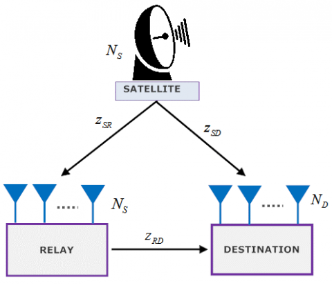
We consider a HSTCN employing MIMO STBC S-DF relaying protocol, where earth stations (terrestrial relay nodes) with antennas selectively forwards the data received from the satellite to the destination. The schematic representation of HSTCN system is shown in Figure 1.
Figure 1. Schematic representation of HSTCN
In this work, we consider time-selective fading channel due to node mobility and imperfect CSI conditions. We assume all the fading channel links are time-selective in nature. Also, we assume links will not vary for one STBC to another STBC codeword matrix. It differs in a time-selective way from one STBC codeword to another STBC codeword within a block. Moreover, in contrast to previous papers (Varshney and Puri, 2017), the presence of a direct SD fading link with an elevation angle $\theta_{S D}$ is also assumed. The elevation angle for the fading link between SR is denoted by $\theta_{S R_{r}}$, where $r=1,2,3, \dots, K$. The time selective MIMO fading links can be modeled using first order autoregressive channel model (AR1) as (Varshnet and Hagannatham, 2017),
$\mathbb{Z}_{i}(p)=v_{i} \mathbb{Z}_{i}(p-1)+\sqrt{1-v_{i}^{2}} E_{i}(p) ; i \in\left\{S D, S R_{r}, R_{r} D\right\}$ (1)
Where the terms $v_{S D}, v_{S R_{r}}$ and $v_{R, P}$ denote the correlation coefficients for the SD, SR and RD faing links respectively. These correlation coefficients can be evaluated $( .)$ using. Jakes. model-as, $v=J_{0}\left(2 \Pi f f_{c} v / R_{s} c\right)$ , where $v_{p}, R_{s}, T_{S}=1 / R_{s}, c, f_{c}$ and $J_{J}( .)$ denote the relative velocity, symbol transmission rate, number of time sloss, speed of $f$ light, carrier frequency and -zeroth-order- Bessel-function of the 1 st-kind-respectively. The random process $E_{i}(p)$ denotes the time-selective component of the associated link, distributed as 'zero mean circular shift complex. Gaussian 'noise. (ZMCSCG) $\left\{i . e ., \sim \mathbb{C} \mathbb{N}\left(0, \sigma_{\varepsilon_{i}}^{2}\right)\right\}$ - In this system- model, we consider that the DN -employs -low complexity. maimal-ratio-combiner. (MRC) receiver. It it is difficult to get instantaneous CSI corresponding to the transmission of every. STBC codeword due to the time-selective nature of the fading links. Thence, like works we assume imperfect $\left.\text { CSI at the } r^{t h} \text { relay node( } \mathrm{RN}\right)$ and $\mathrm{DN} .$
The estimated channel matrices for RD, $\mathrm{SR}$ and $\mathrm{SD}$ -links can be written as $\widehat{Z}_{R D}^{(r)}(1)=\mathbb{Z}_{R D}^{(r)}(1)+\mathbb{Z}_{\epsilon_{R D}}^{(r)}(1), \widehat{Z}_{S R}^{(r)}(1)=\mathbb{Z}_{S R}^{(r)}(1)+\mathbb{Z}_{\epsilon_{S R}}^{(r)}(1) \cdot \quad$ and $. \quad \widehat{Z}_{S D}(1)=$ $\mathrm{Z}_{S D}(1)+\mathrm{Z}_{\epsilon_{S D}}(1)$ respectively, estimated at the beginning of 'each block and in this way used to detect each STBC codeword $X_{S}(p), 1 \leq p \leq M_{b}$ in the consequent block. The $\cdot$ MIMO channel. matrices $Z_{S R_{r}}^{(r)}(1) \in \mathbb{C}^{N \times N}, Z_{R_{r} D}^{(r)}(1) \in \mathbb{C}^{N_{D} \times N}$ and $\cdot Z_{S D}(1) \in$ $\mathbb{C}^{N_{D} \times N}$ . comprised of entries $h_{l, m}^{\left(S R_{r}\right)}(p), h_{n, l}^{\left(R_{r} D\right)}(p) \cdot$ and $\cdot h_{n, m}^{(S, D)}(p) \cdot$ which $\cdot$ are ZMCSCG with variance. $\left(\delta_{S R}^{(r)}\right)^{2},\left(\delta_{R D}^{(r)}\right)^{2}\left(\delta_{S R}^{(r)}\right)^{2},\left(\delta_{R D}^{(r)}\right)^{2}$ and $\delta_{S D}^{2}$ . respectively. The channel-error matrices $\mathbb{Z}_{E_{S R}}^{(1)}(1), Z_{E_{S D}}(1)$ and $\mathbb{Z}_{E_{R D}}^{(r)}(1)$ comprise of entries, which are $\cdot$ ZMCSCG * with \cdotvariance $\cdot\left(\sigma_{E R}^{(r)}\right)^{2}, \sigma_{\epsilon_{S D}}^{2}$ and $\cdot\left(\sigma_{E_{R D}}^{(r)}\right)^{2}$ -respectively. By using $\cdot(1)$ $Z_{S D}(p)$ can be modeled as,
$\mathbb{Z}_{s D}(p)=v_{S D}^{p-1} \hat{\mathbb{Z}}_{s D}(1)-v_{S D}^{p-1} \mathbb{Z}_{\epsilon_{s D}}(1)+\sqrt{1-v_{S D}^{2}} \sum_{i=1}^{p-1} v_{S D}^{p-i-1} E_{S D}(i)$ (2)
Let $N_{D}$ and $N_{S}$ are the number of antennas employed at the DN and satellite node (SN) respectively. In order to keep the data rate of the $S R$ tink same as that of the $\mathrm{RD}$ link, we 'employ the 'same $\cdot \mathrm{S}$ TBC at the $\mathrm{RN}$ and $\mathrm{SN}$ . This also 'means that $N_{R}=N_{S}=$ $N \cdot$ The \cdotMIMO\cdot STBC. S-DF\cdot based\cdot HSTCN\cdotrelaying system\cdotcan be described as. follows. Let.C $=\left\{X_{j}[p]\right\}$ 'denotes the $\cdot \mathrm{STBC}$ \cdotcodeword 'set, where 'each codeword of the \cdotset $C$ is : expressed $\cdot \mathrm{as}, X_{j}(p) \in \mathbb{C}^{N \times T_{S}}$ . and $1 \leq j \leq|C|,$ where. $|C|$ denotes the cardinality of the codeword 'set $C .$ The received symbol -block at the DN-in case of direct SD transmission mode is modeled as,
$Y_{S D}[p]=\sqrt{P_{S} / N R_{C}} v_{S D}^{p-1} \hat{\mathbb{Z}}_{S D}[1] X_{S}[p]+\tilde{W}_{S D}[p]$ (3)
Where $P_{S}, N$ and $R_{C}$ 'denote the total available power budget at the SN, number of antennas at the $S N$ and $S$ TBC code-rate-respectively. For cooperation mode, the received symbol blocks at the RN. and DNN can be modeled as, $\cdots$ .
$Y_{S R}^{(r)}[p]=\sqrt{P_{S} / N R_{C}} v_{S R_{r}}^{p-1}\left(\mathbb{Z}_{S R}^{(r)}[1]+\mathbb{Z}_{\epsilon_{S R}}^{(r)}[1]\right) X_{S}[p]+\tilde{W}_{S R}^{(r)}[p]$ (4)
$Y_{R D}^{(r)}[p]=\sqrt{\tilde{P}_{r} / N R_{C}} v_{R_{r} D}^{p-1}\left(\mathbb{Z}_{R D}^{(r)}[1]+\mathbb{Z}_{\epsilon_{R D}}^{(r)}[1]\right) X_{S}[p]+\tilde{W}_{R D}^{(r)}[p]$ (5)
Where,
$\left\{\begin{aligned} \tilde{P}_{r} &=P_{r} ; \text { if relayrdecodesthesymbolcorrecly } \\ \tilde{P}_{r} &=0 ; \text { ifrelayrdecodesthesymbolincorrecly} \end{aligned}\right.$
$\operatorname{In}(4), P_{r}$ denotes the power available at the $r^{t h}$ relay
The channel noise matrices $\tilde{W}_{S D}[p], \tilde{W}_{S R}^{(r)}[p]$ and $\tilde{W}_{R D}^{(r)}[p]$ comprise of noise terms emerging because of the mobile nodes and imperfect CSI respectively. The effective noise variances $N_{S D}, N_{S R}^{(r)}$ and $N_{R D}^{(r)}$ for $\mathrm{SD}, \mathrm{SR}$ and $\mathrm{RD}$ links can be modeled as,
$N_{S D}=N_{0}+P_{S}\left(N R_{C}\right)^{-1} v_{S D}^{2(p-1)} N_{a} \sigma_{\epsilon_{S D}}^{2}+P_{S}\left(N R_{C}\right)^{-1}\left(1-v_{S D}^{2(p-1)}\right) N_{a} \sigma_{e S D}^{2}$
$N_{S R}^{(r)}=N_{0}+P_{S}\left(N R_{C}\right)^{-1} v_{S R_{r}}^{2(p-1)} N_{a}\left(\sigma_{\mathrm{egR}}^{(r)}\right)^{2}+P_{S}\left(N R_{C}\right)^{-1}\left(1-v_{S R_{r}}^{2(p-1)}\right) N_{a}\left(\sigma_{e_{S R}}^{(r)}\right)^{2}$
$N_{R D}^{(r)}=N_{0}+\tilde{P}_{r}\left(N R_{c}\right)^{-1} v_{R, D}^{2(p-1)} N_{a}\left(\sigma_{E_{D D}}^{(r)}\right)^{2}+\tilde{P}_{r}\left(N R_{C}\right)^{-1}\left(1-v_{R, D}^{2(p-1)}\right) N_{a}\left(\sigma_{e_{D D}}^{(r)}\right)^{2}$ (6)
respectively. Where $N_{a}$ denotes the number of non-zero M-PSK symbols transmitted per codeword. The advantage of using STBC code-word is that, it orthogonalizes the vector channel into a constant scalar channel by creating virtual parallel paths. The effective instantaneous signal to noise ratio (SNR) $\gamma_{S D}(p), \gamma_{S R}^{(r)}$ and $\gamma_{R D}^{(r)}(p)$ for the $\mathrm{SD}, \mathrm{SR}$ and $\mathrm{RD}$ fading links respectively can be modeled as,
$\gamma_{S D}(p)=\frac{P_{S} v_{s D}^{2(p-1)}\left\|\hat{\mathbb{Z}}_{s D}(1)\left(X_{S}(p)-X_{j}(p)\right)\right\|_{F}^{2}}{2 N R_{C} N_{S D}}=C_{S D}(p)\left\|\hat{\mathbb{Z}}_{S D}(1)\right\|_{F}^{2}$
$\gamma_{S R}^{(r)}(p)=\frac{P_{S} U_{S R}^{2(p-1)}\left\|\hat{\mathbb{Z}}_{S R}^{(r)}(1)\left(X_{S}(p)-X_{j}(p)\right)\right\|_{F}^{2}}{2 N R_{C} N_{S R}^{(r)}}=C_{S R}^{(r)}(p)\left\|\hat{\mathbb{Z}}_{S R}^{(r)}(1)\right\|_{F}^{2}$
$\gamma_{R D}^{(r)}(p)=\frac{\tilde{P}_{r} v_{R, D}^{p-1}\left\|\hat{\mathbb{Z}}_{R D}^{(r)}(1)\left(X_{S}(p)-X_{j}(p)\right)\right\|_{F}^{2}}{2 N R_{C} N_{R D}^{(r)}}=C_{R D}^{(r)}(p)\left\|\hat{\mathbb{Z}}_{R D}^{(r)}(1)\right\|_{F}^{2}$ (7)
The effective. SNRs $\gamma_{S D}(p), \gamma_{S R}^{(r)}(p)$ and $\gamma_{R D}^{(r)}(p) \cdot \gamma_{R D}^{(r)}(p)$ are -Gamma distributed in nature, having a cumulative distribution function $(\mathrm{CDF})$ and probability distribution function $(\mathrm{PDF})$ are modeled as,
$F_{\gamma}(t)=\gamma(\Theta, \Lambda t)\{\Gamma(\Theta)\}^{-1}, f_{\gamma}(t)=\wedge^{\ominus} t^{\Theta-1}\{\Gamma(\Theta)\}^{-1} e^{-\Lambda t}$ (8)
Where $\gamma( . . .)$ denotes the lower incomplete - Gamma fiunction and the quantities $(\theta, \Lambda)$ will. be equal. $\mathrm{to} \cdot\left[N N_{D},\left\{C_{S D}(p) \tilde{\delta}_{S D}^{2}\right\}^{-1}\right],\left[N^{2},\left\{C_{S R}^{(r)}(p)\left(\tilde{\delta}_{S R}^{(r)}\right)^{2}\right\}^{2}\right]$ and $\left[N N_{D},\left\{C_{R D}^{(r)}(p)\left(\tilde{\delta}_{R D}^{(r)}\right)^{2}\right\}^{-1}\right]$ for the $S R,$ sD, and $\mathrm{RD}$ . SNR's respectively. Where
$C_{S D}(p), C_{S R}^{(r)}(p)$ and $C_{R D}^{(r)}(p)$ are given as
$C_{\mathcal{B}}(p)=\left\{\overline{\gamma}_{\mathcal{S} D} v_{S D}^{2 p-1}\left(N R_{C}\right)^{-1}\right\}\left\{1+\overline{\gamma}_{\mathcal{B D}}\left(N R_{C}\right)^{-1} \nu_{S D}^{2(p-1)} \tilde{\sigma}_{\epsilon_{\mathcal{D}}}^{2}+\overline{\gamma}_{S D}\left(N R_{C}\right)^{-1}\left(1-\nu_{S D}^{2(p-1)}\right) \tilde{\sigma}_{e_{\mathcal{D}}}^{2}\right\}^{-1}$
$C_{\Re}^{(r)}(p)=\left\{\overline{\gamma}_{S R} v_{S R}^{2(p-1)}\left(N R_{C}\right)^{-1}\right\}\left\{1+\overline{\gamma}_{S R}\left(N R_{C}\right)^{-1} v_{S R}^{2(p-1)}\left(\tilde{\sigma}_{\operatorname{se}}^{(r)}\right)^{2}+\overline{\gamma}_{S R}\left(N R_{C}\right)^{-1}\left(1-v_{S R}^{2(p-1)}\right)\left(\tilde{\sigma}_{e_{S R}}^{(r)}\right)^{2}\right\}^{-1}$
$C_{R D}^{(r)}(p)=\left\{\overline{\gamma}_{R D} v_{R, D}^{p-1}\left(N R_{C}\right)^{-1}\right\}\left\{1+\overline{\gamma}_{R D}\left(N R_{C}\right)^{-1} \mathcal{V}_{R, D}^{p-1} \tilde{\sigma}_{\in D}^{2}+\overline{\gamma}_{R D}\left(N R_{C}\right)^{-1}\left(1-\mathcal{U}_{R, D}^{p-1}\right) \tilde{\sigma}_{e_{R D}}^{2}\right\}^{-1}$
(9)
respectively.
The quantities $\left(\tilde{\sigma}_{\in S R}^{(r)}\right)^{2},\left(\tilde{\sigma}_{S R}^{(r)}\right)^{2},\left(\tilde{\sigma}_{\epsilon_{R D}}^{(r)}\right)^{2}$ and $\left(\tilde{\sigma}_{e_{R D}}^{(r)}\right)^{2}$ are equivalent to $N_{a}\left(\sigma_{E_{S R}}^{(r)}\right)^{2}, N_{a}\left(\sigma_{e_{S R}}^{(r)}\right)^{2}, N_{a}\left(\sigma_{E D}^{(r)}\right)^{2}$ and $\cdot N_{a}\left(\sigma_{e_{R D}}^{(r)}\right)^{2}$ -respectively.
The parameters $\overline{\gamma}_{S R}, \overline{\gamma}_{R D} \cdot \overline{\gamma}_{S R}, \overline{\gamma}_{R D}$ and $\overline{\gamma}_{S D}$ are given as $\overline{\gamma}_{S R}=P_{S} / N_{0}, \overline{\gamma}_{R D}=P_{r} /$ $N_{0} \cdot$ and $\cdot \overline{\gamma}_{S D}=P_{S} / N_{0} \cdot$ respectively. The - quantities $\left(\tilde{\delta}_{S R}^{(r)}\right)^{2}, \tilde{\delta}^{2}_{S D} \cdot$ and $\cdot\left(\tilde{\delta}_{R D}^{(r)}\right)^{2} \cdot$ are defined $\cdot$ as, $\left(\tilde{\delta}_{S R}^{(r)}\right)^{2}=\left(\delta_{S R}^{(r)}\right)^{2}+\left(\sigma_{E_{S R}}^{(r)}\right)^{2}, \tilde{\delta}^{2}_{S D}=\delta_{S D}^{2}+\sigma_{\epsilon_{S D}}^{2} \cdot$ and $\cdot\left(\tilde{\delta}_{R D}^{(r)}\right)^{2}=$ $\left(\delta_{R D}^{(r)}\right)^{2}+\left(\sigma_{\epsilon_{R D}}^{(r)}\right)^{2} \cdot$ respectively. The $\cdot$ terms $\cdot \tilde{\sigma}_{\epsilon S D}^{2}$ . and $\cdot \tilde{\sigma}_{e_{S D} . \text { are equivalent }}^{2}$ to $\operatorname{Na} \sigma_{\in S D}^{2}$ and $\cdot N a \sigma_{e_{S D}}^{2},$ ' respectively, $\lambda_{l 1}, \lambda_{l 2}, \ldots, \lambda_{l N}$ ' represents the singular. values. (SVs) obtained after performing the \cdot singular value decomposition. (SVD) of the STBC codeword. difference $\cdot X_{S}(p)-X_{j}(p), \tilde{h}_{\tilde{l}, n}^{S D} \cdot$ represents the $\cdot(\tilde{l}, n) \cdot$ coefficient of $\cdot$ the $\operatorname{matrix} \approx \widetilde{\mathbb{Z}}_{S D}(1)=\widehat{\mathbb{Z}}_{S D}(1) U_{j}$ for $1 \leq \tilde{l}, n \leq N \cdot \operatorname{and} \cdot U_{j} \in \mathbb{C}^{N \times N}$ is a unitary matrix, i.e., $U_{j} U=U U_{j}=I_{N \times N}$ and for Alamouti-STBC, $\lambda_{l 1}=\lambda_{l 2}=\ldots=\lambda_{l N}=\lambda$In this work we consider that SR and SD fading links are distributed as Shadowed-Rician and RD fading links are modeled as Nakagami-m fading channels. The SR channel matrix $H_{S R}[p] \in \mathbb{C}^{N_{S} \times N_{R}}$ contains independent and identically distributed (i.i.d.) Shadowed-Rician random variables (RVs), can be expressed as,
$\mathbb{Z}_{S R}^{(r)}(p)=\underbrace{\overline{\mathbb{Z}}_{S R}^{(r)}(p)}_{\text {LOS COMPONENT }}+\underbrace{\tilde{\mathbb{Z}}_{S R}^{(r)}(p)}_{\text {SCATTERD COMPONENT }}$ (10)
The minimum antenna spacing for uncorrelated multipath scattered waves is $\cdot \lambda / 2,$ where $\lambda$ denotes the wavelength. Very dense surrounding environment plays an important role in the correlation of the scatter component. Following the system model given in, the channel coefficients of LOS component $\overline{Z}_{S R}^{(r)}(p)$ are i.i.d. Nakagami-mi as RVs with variance $\Omega_{i}$ where mi denotes the shape parameter and its values ranges from 0.50 to $\infty$. The scatter component channel matrix $\widetilde{\mathbb{Z}}_{S R}^{(r)}(p)$ is comprised of entries which are distributed as i.i.d. complex Gaussian RVs with zero average value and variance 2bi.
The instantaneous received SNR for SR link is modeled as,
$\left(\gamma_{S R}^{(r)}(p)\right)^{i}=\left(C_{S R}^{(r)}(p)\right)^{i}\left\|\left(\hat{\mathbb{Z}}_{S R}^{(r)}[1]\right)^{i}\right\|^{2} ; \quad i=1,2, \ldots, N_{S} N_{R}$ (11)
By employing M-PSK modulation, the average PEP for the SR link is modeled as
$P_{E}^{S \rightarrow R}\left(\left(C_{S R}^{(r)}(p)\right)^{i}, m_{i}, \Omega_{i}\right) \cong \xi_{M} \sum_{k=1}^{\eta M}\left(\sum_{i=1}^{N_{s} N_{R}} p_{E}^{S \rightarrow R}\left(\left(C_{S R}^{(r)}(p)\right)^{i}, m_{i}, \Omega_{i}, k\right)\right)$ (12)
Where
$p_{E}^{S \rightarrow R}\left(\left(C_{S R}^{(r)}(p)\right)^{i}, m_{i}, \Omega_{i}, k\right)=\int_{0}^{\infty} Q(\sqrt{g_{k} x}) f_{\left(\gamma_{S R}^{(r)}(p)\right)^{i}}(x) d x$ (13)
Q(⋅) denotes the Q-function which is the tail probability of the Gaussian PDF; modulation specific parameters are defined as: $\xi_{M}=2 / \max \left(\log _{2} M, 2\right), \eta M=\max (M / 4,1)$. Also, max{⋅,⋅} selects greatest of the two positive integers; $\left(\gamma_{S R}(p)\right)^{i} \cdot \operatorname{and} \cdot C_{S R}^{i}(p)$ denote the instantaneous and average SNR, respectively, for the SR link, and $f_{\left(\gamma_{S R}^{(r)}(p)\right)^{i}}(x)$ denotes PDF of $\left(\gamma_{S R}^{(r)}(p)\right)^{i}$.
In Appendix A, it is presented that the PDF of $\left(\gamma_{S R}^{(r)}(p)\right)^{i}$ is modeled as,
$f_{\left(\gamma_{\overline{S} \hat{\boldsymbol{\beta}}}^{(p))}\right.}(x) \cong \alpha_{i}^{N_{i}} \sum_{i_{i}}^{c_{i}}\left(\begin{array}{c}{c_{i}} \\ {l_{i}}\end{array}\right) \beta_{i}^{c_{i}-l_{i}}\left(\begin{array}{c}{J\left(x, l_{i}, d_{i},\left(C_{S R}^{(r)}(p)\right)^{i}\right)} \\ {+\epsilon_{i} \delta_{i} J\left(x, l_{i}, d_{i}+1,\left(C_{S R}^{(r)}(p)\right)^{i}\right)}\end{array}\right)$(14)
Where
$\begin{aligned} J\left(x, l_{i}, d_{i},\left(C_{S R}^{(r)}(p)\right)^{j}\right)=& \frac{x^{d_{i}-l-1}}{\left.\left\{\left(C_{S R}^{(r)}(p)\right)^{i}\right\}^{i}\right\}^{(i-l)} \Gamma\left(d_{i}-l_{i}\right)} \\ & \times_{1} F_{1}\left(d_{i} ; d_{i}-l_{i} ;-\frac{\left(\beta_{i}-\delta_{i}\right) x}{\left(C_{S R}^{(p)}(p)\right)^{i}}\right) \end{aligned}$ (15)
$\alpha_{i}=0.5\left(2 b_{i} m_{i} /\left(2 b_{i} m_{i}+\Omega_{i}\right)\right)^{m_{i}} / b_{i}, \beta_{i}=\left(0.5 / b_{i}\right), \delta_{i}=0.5 \Omega_{i} /\left(2 b_{i}^{2} m_{i}+\right.$ $\left.b_{i} \Omega_{i}\right), 2 b_{i}$ denotes the multipath component’s average power,$\cdot c_{i}=\left(d_{i}-N_{i}\right)^{+}, \epsilon_{i}=m_{i} N_{i}-d_{i}, d_{i}=\max \left\{N_{i},\left[m_{i} N_{i}\right]\right\}$ and $|z|$ denotes the largest integer not greater than $\tau ;(Z)^{+}$ indicates that if $\tau$ - $z \leq 0,$ then use $-2=0 ; z=0$ ; $\Gamma(\cdot) \cdot$ denotes the Gamma function, and $-1 F_{1}( ; ; \text { ; } .)$ denotes the confluent
hypergeometric function.
Substituting (14) in (13), we obtain,
$p_{E}^{S \rightarrow R}\left(\left(C_{S R}^{(r)}(p)\right)^{i}, m_{i}, \Omega_{i}, k\right) \cong$ $\alpha_{i}^{N_{i}} \sum_{i=0}^{c_{i}}\left(l_{i}^{c_{i}-l_{i}} \times\left(\kappa\left(l_{i}, d_{i},\left(C_{S R}^{(r)}(p)\right)^{i}, k\right)+\epsilon_{i} \delta_{i} \kappa\left(l_{i} d_{i}+1,\left(C_{S R}^{(r)}(p)\right)^{i}, k\right)\right)\right.$ (16)
Where,
$\kappa\left(l_{i}, d_{i},\left(\gamma_{S R}^{(r)}(p)\right)^{i}, k\right)=$
$\frac{1}{\left\{\left(\gamma_{S S}^{(r)}(p)\right)^{r d-l_{i}} \Gamma\left(d_{i}-l_{i}\right)\right.} \int_{0}^{\infty} x^{d_{i}-l_{i}-1} Q(\sqrt{g_{k} x}) \times_{1} F_{1}\left(d_{i} ; d_{i}-l_{i} ;-\frac{\left(\beta_{i}-\delta_{i}\right) x}{\left(C_{S R}^{(r)}(p)\right)^{i}}\right) d x$ (17)
Using the relation given in $Q(\sqrt{g_{k} x})$ can be written as,
$Q(\sqrt{g_{k} x})=\frac{1}{2} \operatorname{erfc}(\sqrt{\frac{g_{k} x}{2}})=\frac{1}{2 \sqrt{\pi}} G_{12}^{20}\left(\frac{g_{k} x}{2} | \begin{array}{c}{1} \\ {0,1 / 2}\end{array}\right)$ (18)
$F_{1} F_{1}\left(d_{i} ; d_{i}-l_{i} ;-\frac{\left(\beta_{i}-\delta_{i}\right) x}{\left(C_{S R}^{(r)}(p)\right)^{i}}\right)=\frac{\Gamma\left(d_{i}-l_{i}\right)}{\Gamma\left(d_{i}\right)} G_{12}^{11}\left(\frac{\left(\beta_{i}-\delta_{i}\right) x}{\left(C_{S R}^{(r)}(p)\right)^{i}} | \begin{array}{c}{1-d_{i}} \\ {0,1-d_{i}+l_{i}}\end{array}\right)$ (19)
Where $\operatorname{erfc}(\cdot)$ and $G_{p, q}^{m, n}$ denote the complementary error function and Meijer-G function respectively.
Substituting (18) and (19) into (17), $\kappa\left(l_{i}, d_{i},\left(C_{S R}^{(r)}(p)\right)^{i}, k\right)$ is given as,
$\kappa\left(l_{i}, d_{i},\left(C_{S R}^{(r)}(p)\right)^{i}, k\right)=$
$\frac{2^{d_{i}-l_{i}-1}}{2 \sqrt{\pi} \Gamma\left(d_{i}\right)\left(\left(C_{S R}^{(r)}(p)\right)^{i}\right)^{d_{i}-l_{i}}} \int_{0}^{\infty} x^{d_{i}-l_{i}-1} G_{12}^{2}$
$G_{12}^{2}\left(\frac{g_{k} x}{2} | \begin{array}{c}{1} \\ {0,1 / 2}\end{array}\right)$
$G_{12}^{11}\left(\frac{\left(\beta_{i}-\delta_{i}\right) x}{\left(C_{S R}^{(r)}(p)\right)^{i}} | \begin{array}{c}{1} \\ {0,1 / 2}\end{array}\right)$dx (20)
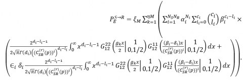
The PEP for SR link can be obtained by substituting (16) into (12), as given below,
(21)
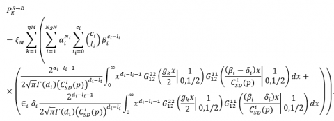
Following the similar approach, the PEP for the SD link can be written as,
(22)
Instantaneous PEP for the event when $X_{S}[p] \in \mathbb{C}^{N \times T_{S}}$ is transmitted and $X_{j}[p] \in \mathbb{C}^{N \times T_{S}}$ is detected conditioned on the RD fading link instantaneous SNR $\gamma_{R D}^{(r)}(p)$ is modeled as,
$P_{R \rightarrow D}\left(X_{S}[p] \rightarrow X_{j}[p] / \gamma_{R D}^{(r)}(p)\right)=Q(\sqrt{2 \gamma_{R D}^{(r)}(p)})$ (23)
Where $Q( .)$ denotes the Gaussian $Q$ function, it is the area under the tail of a Gaussian curve, defined as, $Q(h)=\frac{1}{\sqrt{2 p i}} \int_{\hbar}^{\infty} \exp \left(-u^{2} / 2\right) d u .$ Average $\mathrm{PEP}$ $P_{R \rightarrow D}\left(X_{S}[p] \rightarrow X_{j}[p]\right)$ be derived by averaging $(23)$ over the PDF of $\gamma_{R D}^{(r)}(p),$ we use the MGF based approach. It can be modeled as,
$P_{R \rightarrow D}\left(X_{S}[k] \rightarrow X_{j}[k]\right)=\frac{1}{p i} \int_{0}^{p i / 2} M_{\gamma_{R D}(p)}\left[1 / \sin ^{2}(\theta)\right] d \theta$ (24)
Where $M_{\gamma_{R D}^{(r)}(p)}( .)$ denotes the MGF and is modeled as,
$M_{\gamma, \beta \delta(p)}\left[1 / \sin ^{2}(\theta)\right]=\left(\frac{1}{1+\frac{\lambda_{j}^{2} C_{R D}^{(p)}(p)\left(\tilde{\delta}_{R D}^{(r)}\right)^{2}}{m_{R D} N_{D} N \sin ^{2}(\theta)}}\right)^{\left(m_{m} N_{D}, N\right)}$ (25)
Following the detailed solution of (25) given in Appendix B, the average PEP for RD link is modeled as,
$P_{R \rightarrow D}\left(X_{S}[p] \rightarrow X_{j}[p]\right)=\frac{1}{2 p i}\left(\frac{1}{1+\frac{\lambda^{2} C_{P D}^{(r)}}{M_{R D} N_{D} N \sin ^{2}(\theta)}}\right)^{m_{D} N_{D} N}$
$\underset{x_{2}}{_{2}} F_{1}\left[m_{P D} N_{D} N, 0.50, m_{P D} N_{D} N+1 ; 1-\frac{1}{\left.1+\frac{\lambda^{2} C_{P D}^{(T)}(p)\left(\tilde{\delta}_{P D}^{(r)}\right)^{2}}{m_{P D} N_{D} N}\right]}\right]$ (26)
The average PEP union bound can write as the summation of all PEP terms over the STBC codes $X_{j}[p] \in C \mathrm{as}$,
$P_{R \rightarrow D}[p] \leq \sum_{X,[p] \leq C, X_{j}|p| \times X_{S}[p]} P_{R \rightarrow D}\left(X_{S}[p] \rightarrow X_{j}[p]\right)$ (27)
In relaying phase when relay correctly decodes the signal received from the source node then at the destination, we get the signal path from the source node as well as from the relay node. Using (22) and (27), the average PEP for cooperation modes,
$P_{S \rightarrow D, R \rightarrow D}[k]$ can be written as,(28)
Therefore, the end-to-end PEP for HSTCN system can be written as,
$P_{E}=P_{E}^{S \rightarrow R} \times P_{E}^{S \rightarrow D}+P_{S \rightarrow D, R \rightarrow D}[k] \times\left(1-P_{E}^{S \rightarrow R}\right)$ (29)
Substituting (28), (22) and (21) into (29), we will get the end-to-end PEP for HSTCN system.
The HSTCN system performance can be easily understood by assuming high SNR regimes. Coding gain (CG) and diversity gain (DG) are the two important parameters which help in analyzing the PEP performance of the system. CG is the measure in the difference between the SNR levels between the uncoded system and coded system required to reach the same PEP levels when used with the error correcting code (ECC). DG is the increase in signal-to-interference (SINR) ratio due to some diversity scheme, or how much the transmission power can be reduced when a diversity scheme is introduced, without a performance loss. DG is usually expressed in decibels, and sometimes as a power ratio. In general, the asymptotic value of the PEP can be written as,
$\lim _{x \rightarrow \infty} P_{E} \approx \frac{(C G)^{-D G}}{\overline{\gamma}^{D G}}$ (30)
Where $\overline{\gamma}$ denotes the average SNR. The average PEP expression is expressed in terms of Meijer- $G$ function. To find the system's asymptotic PEP, we need to find the asymptotic value of the Major-G function. For $\left(C_{S R}^{(r)}(p)\right)^{i} \rightarrow \infty$ and $C_{S D}^{i}(p)$ asymptotically tight expression for Meijer- $G$ function is given as,
$G_{33}^{13}\left(\frac{2\left(\beta_{i}-\delta_{i}\right)}{C_{S D}^{\prime}(p) g_{k}} | \begin{array}{c}{1-d_{i}, 1-d_{i}+l_{i}, 1 / 2-d_{i}+l_{i}} \\ {0,-d_{i}+l_{i},-d_{i}+l_{i}}\end{array}\right) \rightarrow \frac{\Gamma\left(d_{i}\right) \Gamma\left(d_{i}-l_{i}+1 / 2\right)}{\Gamma\left(d_{i}-l_{i}+1\right)}$ (31)
At very high SNR, the term containing the product of probabilities can be ignored in (29). In addition, by using (31), assuming that $C_{S D}(p)=C_{S D}^{i}(p)$ and after some algebra, we can write the asymptotic average PEP of the system as,
$p_{e}\left(C_{s D}(p), m_{i}, \Omega_{i}\right) \cong \xi_{M} \sum_{i=1}^{2} p_{e_{i}}\left(C_{s D}(p), m_{i}, \Omega_{i}\right)$ (32)
Where,
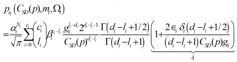
(33)
For very large CsD , in (33), the term For very large , in (33), the term ; therefore, we obtain [ ],
$\lim _{C_{S D}(p) \rightarrow \infty} p_{e_{i}}\left(C_{S D}(p), m_{i}, \Omega_{i}\right)$
$=\frac{\alpha_{i}^{N_{i}}}{\sqrt{\pi}} \sum_{i=0}^{c_{i}}\left(\begin{array}{c}{c_{i}} \\ {l_{i}}\end{array}\right) \beta_{i}^{c_{i}-l_{i}} g_{1}^{l_{i}-d_{i}} 2^{d_{i}-l_{i}-1} \frac{\Gamma\left(d_{i}-l_{i}+1 / 2\right)}{\Gamma\left(d_{i}-l_{i}+1\right)} \frac{1}{C_{S D}(p)^{d_{i}-l_{i}}}$ (34)
At very high SNR, the decay of the term $p_{e_{i}}\left(C_{S D}(p), m_{i}, \Omega_{i}\right)$ is dominated by the lowest power of $C_{S D}(p) ;$ therefore, after some algebra, we obtain the asymptotic PEP of the considered scheme from $(33)$ and $(34),$ i.e.
$\begin{aligned} \lim _{C_{\mathfrak{B}}(p) \rightarrow \infty} p_{e}\left(C_{S D}(p), m_{f}, \Omega_{7}\right) & \cong \frac{\xi_{M} \alpha_{1}^{N_{5}} \Gamma\left(N_{S}+1 / 2\right) g_{1}^{-N_{D}} 2^{N_{5}-1}}{\sqrt{\pi} \Gamma\left(N_{S}+1\right)} \frac{1}{C_{S D}(p)^{N_{S}}} \\ &+\frac{\xi_{M} \alpha_{2}^{N_{2}} \Gamma\left(N_{D}+1 / 2\right) g_{1}^{-N_{D}} 2^{N_{D}-1}}{\sqrt{\pi}\left(N_{D}+1\right)} \frac{1}{C_{S D}(p)^{N_{D}}} \end{aligned}$ (35)
It can be seen from (35) that the DO of the satellite relay system is $\min \left\{N_{S}, N_{D}\right\}+N N_{D}$. This result indicates that if the relay has NR transmit antenna, then no diversity gain can be chieved in the HSTCN by installing multiple antennas at the destination Earth station. Similarly, if the destination has ND receive antenna, then it will experience no diversity gain due the MIMO based source Earth station. Hence, to experience the diversity advantage, the source and the destination must use multiple antennas, i.e., Ni>1 .
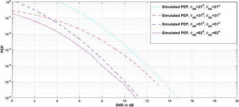
Simulations have been conducted in various conditions of node mobility over time varying channel. Simulation parameters are given as, M=4, K=2, noise variance This section presents simulation results to demonstrate the performance of the HSTCN relaying network in various mobility scenarios. Figure 2 demonstrates the impact of the satellite elevation angles on the end-to-end PEP performance of the system for a scenario when all the links are quasi-static i.e., $\rho=1$ and all elevation angles equal i.e.,$\theta_{S R_{1}}=\theta_{S R_{2}}=\theta_{S R}$. It can be seen in Figure 2 that increasing the elevation angles results in a significant improvement in the end-to-end performance. This is because high elevation angles lead to favorable channel with infrequent light shadowing (ILS) in satellite-terrestrial links.
Figure 2. PEP versus SNR in dB performance of the MIMO STBC S-DF based HSTCN relaying network for various values of satellite elevation angle with
$\begin{aligned} \theta_{S D}, \theta_{S R_{1}}=\theta_{S R_{2}}=\theta_{S R} & \in\left\{21^{\circ}, 31^{0}, 51^{0}, 82^{0}\right\}, P_{S}=P_{1}=1 / 3, m_{R_{1} D}=\\ m_{R_{2} D}=m_{R D}=0.60 a n d f_{C}=5.9 G H z, R_{C}=9.6 \mathrm{Kbps}, P_{S}=P_{1}=& P_{2}=1 / 3, \rho_{S D}=\\ \rho_{S R_{1}}=\rho_{S R_{2}}=\rho_{R_{1} D}=\rho_{R_{2} D}=\rho \in\{0.9856,0.9889,0.9989\}, \sigma_{e S D}^{2}=\sigma_{e S R_{r}}^{2}=& \sigma_{e S R_{r}}^{2}=\\ \sigma_{e R_{r} D}^{2}=\sigma_{e}^{2}=\{0.09,0.02\} \forall r \end{aligned}$
This paper presents the performance analysis for a selective DF cooperative hybrid satellite-terrestrial system with multiple relays where the satellite-to-relay links experience non-identical time-selective shadowed Rician fading and the relay-destination terrestrial links are assumed to be nonidentical time-selective generalized Nakagami faded. Closed form expressions have been derived for the per-frame average SER and the asymptotic SER floor. Simulation results show the impact of terrestrial node mobility as well as the satellite elevation angles on the end-to-end performance.
Table 1. Lms channel parameters
|
Shadowing |
bi |
mi |
$\Omega_{i}$ |
|
Frequency heavy shadowing |
0.063 |
0.739 |
$8.97 \times 10^{-4}$ |
|
Average shadowing |
0.126 |
10.10 |
0.835 |
|
Infrequent Light Shadowing |
0.158 |
19.40 |
1.29 |
The $j ^ { t h } , j = 1,2 , \ldots , N _ { i }$ entry of $h _ { i }$ is distributed as,
$f _ { \left| h _ { j }^{(i)} \right| ^ { 2 } } ( x ) = \alpha _ { i } e _ { 1 } ^ { - \beta _ { x } } F _ { 1 } \left( m _ { i } ; 1 ; \delta _ { i } x \right) , x > 0$ (36)
The MGF of $\left| h _ { j } ^ { ( i ) } \right| ^ { 2 }$ can be expressed as,
$M _ { \left| h _ { j } ^ { ( i ) } \right| ^ { 2 } } ( s ) = E _ { \left| h _ { j } ^ { ( i ) } \right| ^ { 2 } } \left\{ e ^ { - s \left| h _ { j } ^ { ( i ) } \right| ^ { 2 } } \right\} = \int _ { 0 } ^ { \infty } e ^ { - s x } f _ { \left| h _ { j } ^ { ( i ) } \right| ^ { 2 } } ( x ) d x$ (37)
Where $E \{ \cdot \}$ represents the expectation. By using in $( 37 ) ,$ it can be shown that,
$M _ { \left| k _ { j } ^{(i)}\right| ^ { 2 } } ( s ) = \frac { \alpha _ { i } } { \left( s + \beta _ { i } \right) } F \left( m _ { i } , 1 ; 1 ; \frac { \delta _ { i } } { \left( s + \beta _ { i } \right) } \right)$ (38)
where $F ( \alpha , \beta ; \gamma ; z )$ is the Hypergeometric function. Next, by using in $( 38 ) ,$ we get,
$M _ { \left| h _ { j } ^ { ( i ) } \right| ^ { 2 } } ( s ) = \alpha _ { i } \frac { \left( s + \beta _ { i } \right) ^ { m _ { i } - 1 } } { \left( s + \beta _ { i } - \delta _ { i } \right) ^ { m _ { i } } }$ (39)
Under the assumption of i.i.d. entries in $h _ { i }$ , the moment generating function of $\left\| h _ { i } \right\| ^ { 2 }$ can be written as,
$M _ { \| \left. h _ { i } \right| ^ { 2 } } ( s ) = \prod _ { j = 1 } ^ { N _ { i } } M _ { \left| h _ { j } ^ { ( i ) } \right| ^ { 2 } } ( s ) =$ $\alpha _ { i } ^ { N _ { i } } \frac { \left( s + \beta _ { i } \right) ^ { c _ { i } } } { \left( s + \beta _ { i } - \delta _ { i } \right) ^ { d _ { i } } } \left( 1 + \frac { \delta _ { i } } { s + \beta _ { i } - \delta _ { i } } \right) ^ { \varepsilon _ { i } }$ (40)
It can be easily verified from TABLE I that $\beta _ { i } > \delta _ { i }$ for all kinds of shadowing. As $| s | \geq 0 ,$ therefore $\left| \delta _ { i } / \left( s + \beta _ { i } - \delta _ { i } \right) \right| < < 1 .$ since $\varepsilon _ { i } < 1 ,$ an extremely tight (very close to accurate) approximation, $( 1 + z ) ^ { n } \cong 1 + n z , | z | < 1 ,$ can be used in $( 40 ) ,$ to find that,
$M _ { \| h_i \| ^ { 2 } } ( s ) = \alpha _ { i } ^ { N _ { i } } \sum _ { l _ { i } } ^ { c _ { i } } \left( \begin{array} { c } { c _ { i } } \\ { i _ { i } } \end{array} \right) \beta ^ { c _ { i } - l _ { i } } \left( \frac { s ^ { l } } { \left( s + \beta _ { i } - \delta _ { i } \right) ^ { d _ { i } } } + \frac { \varepsilon _ { i } \delta _ { i } s ^ { l _ { i } } } { \left( s + \beta _ { i } - \delta _ { i } \right) ^ { d _ { i } + 1 } } \right)$ (41)
Taking the inverse Laplace transform of (41) and after some algebra, we obtain (16).
To solve $ { I _ { 1 } }$ , let us change the variable by substitution $\cos ^ { 2 } \theta = t$ . This leads to,
$\sin ^ { 2 } \theta = 1 - \cos ^ { 2 } \theta = 1 - t - 2 \cos \theta \sin \theta d \theta = d t$ (42)
Thus, the limits of integral would change from 0 to 1 and the integrating variable dθ changes to
$d \theta = \frac { d t } { - 2 \sqrt { t } \sqrt { 1 - t } }$ (43)
Therefore, $I _ { 1 }$ can now be given as
$I _ { 1 } = \frac { a } { \pi } \int _ { 0 } ^ { 1 } \left( \frac { m N _ { t } N _ { r } } { m N _ { t } N _ { r } + \frac { b \overline { \gamma } } { ( 1 - t ) } } \right) ^ { m N _ { t } N _ { r } } \frac { d t } { 2 \sqrt { t } \sqrt { 1 - t } }$ (44)
After rearrangements and mathematical manipulations, this integral can be represented in the standard form as,
$I _ { 1 } = \frac { a } { 2 \pi } \left( \frac { 2 m N _ { t } N _ { r } } { m N _ { t } N _ { r } + b \overline { \gamma } } \right) ^ { m N _ { t } N _ { r } }$$\int _ { 0 } ^ { 1 } \frac { ( 1 - t ) ^ { m v _ { t } N _ { r } - \frac { 1 } { 2 } } } { \sqrt { t } } \left( 1 - \frac { t } { 1 + \frac { b \overline { \gamma } } { 2 m N _ { t } N _ { r } } } \right) ^ { - m v _ { t } N _ { r } }$ (45)
The above expression represents the integral in the standard form of the Gauss hypergeometric function defined as
$_ 2 F _ { 1 } ( a , b ; c ; x ) = \left. \frac { \Gamma ( c ) } { \Gamma ( c - a ) \Gamma ( a ) } \int _ { 0 } ^ { 1 } t ^ { b - 1 } ( 1 - t ) ^ { c - b - 1 } ( 1 - t x ) \right| ^ { - a } d t$ (46)
Comparing the above definition of the Gauss hypergeometric function with the expression of $I _ { 1 } ,$ the parameters can be obtained as $a = m N _ { t } N _ { r } , b = \frac { 1 } { 2 } , c = m N _ { t } N _ { r } +$ 1and $x = 1 - \frac { 1 } { 1 + \frac { b y } { 2 m N _ { t } N _ { r } } }$ can be given as,
$I _ { 1 } = \frac { a } { 2 \pi } \left( \frac { 2 m N _ { t } N _ { r } } { m N _ { t } N _ { r } + b \overline { \gamma } } \right) ^ { m v _ { t } N _ { r } } \frac { \Gamma \left( m N _ { t } N _ { r } \right) \Gamma \left( \frac { 1 } { 2 } \right) } { \Gamma \left( m N _ { t } N _ { r } + 1 \right) }$ $\times _ { 2 } F _ { 1 } \left( m N _ { t } N _ { r } , \frac { 1 } { 2 } ; m N _ { t } N _ { r } + 1 ; 1 - \frac { 1 } { 1 + \frac { b \overline { \gamma } } { 2 m N _ { t } N _ { r } } } \right)$ (47)
Abdi A., Lau W. C., Alouini M. S., Kaveh M. (2003). A new simple model for land mobile satellite channels: First- and second-order statistics. IEEE Transactions on Wireless Communications, Vol. 2, No. 3, pp. 519-528. https://doi.org/10.1109/TWC.2003.811182
An K., Lin M., Ouyang J., Huang Y., Zheng G. (2014). Symbol error analysis of hybrid satellite–terrestrial cooperative networks with cochannel interference. IEEE Communications Letters, Vol. 18, No. 11, pp. 1947-1950. https://doi.org/10.1109/LCOMM.2014.2361517
Bhatnagar M. R. (2015). Performance evaluation of decode-and-forward satellite relaying. IEEE Transactions on Vehicular Technology, Vol. 64, No. 10, pp. 4827-4833. https://doi.org/10.1109/TVT.2014.2373389
Bhatnagar M. R., Arti M. K. (2013). Performance analysis of af based hybrid satellite-terrestrial cooperative network over generalized fading channels. IEEE Communications Letters, Vol. 17, No. 10, pp. 1912-1915. https://doi.org/10.1109/LCOMM.2013.090313.131079
Gradshteyn I. S., Ryzhik I. M. (2007). Table of Integrals, Series, and Products. https://doi.org/10.2307/2007757
Halber A., Chakravarty D. (2018). Wireless relay placement optimization in underground room and pillar mines. Mathematical Modelling of Engineering Problems, Vol. 5, No. 2, pp. 67-75. https://doi.org/10.18280/mmep.050203
Iqbal A., Ahmed K. M. (2011). A hybrid satellite-terrestrial cooperative network over non identically distributed fading channels. Journal of Communications, Vol. 6, No. 7, pp. 581–589. https://doi.org/10.4304/jcm.6.7.581-589
Iqbal A., Ahmed K. M. (2015). Impact of MIMO enabled relay on the performance of a hybrid satellite-terrestrial system. Telecommunication Systems, Vol. 58, No. 1, pp. 17-31. https://doi.org/10.1007/s11235-014-9864-9
Ruan Y., Li Y., Wang C., Zhang R., Zhang H. (2017). Outage performance of integrated satellite-terrestrial networks with hybrid CCI. IEEE Communications Letters, Vol. 21, No. 7, pp. 1545-1548. https://doi.org/10.1109/LCOMM.2017.2694005
Sharma N., Bansal A., Garg P. (2016). Performance of DF based dual-hop dual-path hybrid RF/FSO cooperative system. Wireless Personal Communications, Vol. 91, No. 2, pp. 1003-1021. https://doi.org/10.1007/s11277-016-3510-7
Sreng S., Escrig B., Boucheret M. (2013). Exact outage probability of a hybrid satellite terrestrial cooperative system with best relay selection. 2013 IEEE International Conference on Communications (ICC), pp. 4520-4524. https://doi.org/10.1109/ICC.2013.6655280
Srikanth B., Kumar H., Rao K. U. M. (2018). A robust approach for WSN localization for underground coal mine monitoring using improved RSSI technique. Mathematical Modelling of Engineering Problems, Vol. 5, No. 3, pp. 225-231. https://doi.org/10.18280/mmep.050314
Varshney N., Jagannatham A. K. (2017). MIMO-STBC based multiple relay cooperative communication over time-selective Rayleigh fading links with imperfect channel estimates. IEEE Transactions on Vehicular Technology, Vol. 66, No. 7, pp. 6009-6025. https://doi.org/10.1109/TVT.2016.2634924
Varshney N., Puri P. (2017). Performance analysis of decode-and-forward-based mixed MIMO-RF/FSO cooperative systems with source mobility and imperfect CSI. Journal of Lightwave Technology, Vol. 35, No. 11, pp. 2070-2077. https://doi.org/10.1109/JLT.2017.2675447
Yang L., Hasna M. O. (2015). Performance analysis of amplify-and-forward hybrid satellite-terrestrial networks with cochannel interference. IEEE Transactions on Communications, Vol. 63, No. 12, pp. 5052-5061. https://doi.org/10.1109/TCOMM.2015.2495278