Padmapriya Krishnamurthy*![]() | Ezhumalai Periyathambi
| Ezhumalai Periyathambi![]()
© 2025 The authors. This article is published by IIETA and is licensed under the CC BY 4.0 license (http://creativecommons.org/licenses/by/4.0/).
OPEN ACCESS
The diagnosis of brain diseases is an emerging research focus that leverages artificial intelligence and multimodal imaging for early and accurate prediction. Functional MRI provides valuable biomarkers for clinical diagnosis, but existing imaging techniques face limitations such as low resolution and difficulty integrating multimodal data. To address this, the proposed research develops an enhanced diagnostic system using a Cross-Modal Super Resolution Graph Adversarial Network (Cross-SRGAN) combined with Hybrid Manifold Learning with Dynamic Weighting (HMLDW). Cross-SRGAN improves the resolution and visual quality of multimodal brain images, including MRI and PET scans, by dynamically learning inter-modal relationships through mutual learning. It is trained using paired low- and high-resolution images with adversarial and perceptual loss functions to reconstruct finer anatomical and structural details critical for disease interpretation. The super-resolved images are then processed by HMLDW, which adaptively extracts both local and global manifold features. This model dynamically adjusts weights of different manifold learning strategies to generate an optimized feature representation. The ensemble features are fed into a Graph Neural Network to classify subjects into normal or disease-affected categories. Experimental performance demonstrates that the hybrid Cross-SRGAN + HMLDW framework delivers higher image fidelity and improved classification accuracy compared to conventional diagnostic approaches.
brain disease diagnosis, functional magnetic resonance imaging, multi-modal data, Cross-SRGAN, HMLDW
One of the most important and intricate organs in the human body is the brain. It is essential for generating ideas, solving problems, reasoning, making decisions, imagining, and remembering, among other functions. Information and experiences can be stored and retrieved from memory. The entirety of our life’s history is preserved in our physical memory plays a crucial role in shaping our identities and character [1]. Memory loss related to dementia and losing our sense of surroundings can be terrifying experiences. Dementia with Alzheimer's disease (AD) is the most common type. As people age, often become more fearful of Alzheimer's. Alzheimer's patients gradually lose the ability to recognize their family members, to love or care for others to follow basic instructions and to connect with the outside world due to the disease's slow but inevitable destruction of brain cells [2].
A person may lose their capacity to breathe, swallow, and cough in more advanced stages. In the 18th largest economy in the world, the expenditures on social and health care for the approximately 50 million people affected by dementia are significant. An estimated 152 million instances of AD and related dementias are expected by 2050 with a new case occurring every three seconds [3]. This represents a significant increase in the number of cases by 2050. The symptoms of AD can also be confused with those of Vascular Dementia (VD) or normal aging, making diagnosis more challenging. Early and precise identification of AD is essential for effective treatment, prevention, and patient care can be accomplished by frequently monitoring its progression [4]. Numerous research programs aim to use brain imaging such as MRIs, to detect AD. MRI can determine the quantity and size of brain cells and may also demonstrate parietal atrophy in cases of AD [5].
In numerous scientific domains, images play an important part, with medical imaging being especially essential in providing significant understanding of brain activity. Methods like neuroimaging, particularly Magnetic Resonance Imaging (MRI), are essential for studying brain anatomy and function and detecting brain illnesses [6]. To diagnose AD dementia, medical professionals evaluate AD signs and symptoms alongside numerous tests. Physicians may recommend memory tests, brain imaging examinations, or other laboratory assessments. These tests assist in diagnosing patients by ruling out illnesses with like symptoms [7]. MRI scans can classify Mild Cognitive Impairment (MCI) patients who may be at risk of increasing AD by detecting brain abnormalities connected with MCI. For instance, in MRI scans used to classify abnormalities, the temporal and parietal lobes are between the brain regions that display size decrease [8]. From brain imaging data, Machine Learning (ML) and Deep Learning (DL) are becoming more and more important for gleaning important insights and forecasting AD. This technological revolution is driven by modern brain imaging methods and the vast amounts of information they generate [9].
To classify cases of AD, a variation of machine-learning methods has been used, with models displaying outstanding results. Traditional learning-based approaches typically comprise three phases: first, determining the brain's Regions of Interest (ROIs); second, choosing features from these ROIs; and third, generating and evaluating classification models [10]. A main challenge with traditional learning-based approaches is the manual selection and extraction of features in feature engineering, which can suggestively impact the model's performance. In recent decades, DL has emerged as a revolutionary method associated to standard ML methods. DL has made feature extraction automatic, removing the necessity for human experts and permitting the procedure to be seamlessly integrated with classification, rather than necessitating manual, different phases [11].
This study presents a unique technique that combines HMLDW with Cross-SRGANs. The Cross-SRGAN framework improves low-resolution neuroimaging data by allowing better feature extraction across numerous imaging modalities. HMLDW progresses the diagnostic procedure by combining adaptive weighting and manifold learning to integrate multi-modal data simultaneously. This combination method purposes to rise the resilience and precision of brain illness diagnosis by efficiently managing large and diverse neuroimaging information [12]. The major contribution of this research:
• To progress an advanced diagnostic system that uses Cross-SR GAN and HMLDW to screen for brain illnesses based on numerous imaging data.
• GANs have been used for the aggregation of multi-modal brain connectomes. Most existing GAN means do not incorporate the correlation between inter-modal relationships.
• The Cross-SR GANs dynamically learn the inter-modal relationships and perform mutual learning.
• HMLDW also helps enhance the assembly of highly informative features, resulting in better classification rates of brain diseases compared to conventional models.
The residual sections of this work are structured as follows: Section 2 reviews related works, Section 3 discusses the proposed technique and its specifics, Section 4 provides an explanation and discussion of the results, and Section 5 presents the conclusion and future recommendations.
GAN-based models have demonstrated strong potential in improving MRI resolution and extracting reliable structural features. One work applied convolutional layers in a GAN framework to classify brain cancers, enabling feature refinement through adversarial learning. It successfully discriminated gliomas, meningiomas, and pituitary tumours using a dataset of 233 patients, achieving high accuracy supported by evaluation metrics such as sensitivity and F1-score [13]. Building on these, segmentation-focused research has leveraged quick thresholding and regional segmentation techniques integrated with transfer learning, where pre-trained networks like AlexNet and VGG-19 were adapted using smaller MRI datasets. These transfer-learning approaches showed improved initialization for tumor segmentation tasks, boosting localization and interpretation performance [14]. Advanced segmentation methods have adopted U-Net variants incorporating attention mechanisms. A multiscale residual attention U-Net effectively emphasized pathological regions while maintaining boundary precision, resulting in superior localization of tumor structures. CNN models trained from scratch on brain MRI datasets showed testing accuracies above 95%, demonstrating that custom architectures can achieve strong performance even without pre-trained initializations. These models often require a large number of annotated samples, which are difficult to collect for low-incidence neurological disorders [15].
To optimize classification efficiency, hybrid boosted models combining multiple feature streams have been introduced. One such model, termed Deep Hybrid Boosted architecture, reached 95% accuracy in MRI-based tumor recognition. Nonetheless, such feature fusion and boosting strategies are computationally intensive and demand expert-driven tuning to ensure stability and consistency across datasets. Feature fusion complexity also increases the risk of overfitting when training data is limited [16]. Multicenter neuroimaging introduces additional domain shift problems due to scanner variability and acquisition differences. To address this, a Multi-Discriminator Active Adversarial Network (MDAAN) was proposed for multi-center brain disorder classification. By jointly learning invariant latent representations across centers and assigning adaptive weights based on sample difficulty, MDAAN effectively reduced negative transfer across imaging sites. This selective labeling strategy decreased annotation cost while maintaining high diagnostic accuracy [17].
Another critical research direction targets the challenge of missing or incomplete multimodal data. A spatially-constrained Fisher representation framework was developed to infer missing PET images from MRI using hybrid GAN architecture. Spatial anatomical constraints enforced consistency between inferred PET signals and individual brain morphology. The technique significantly improved both neuroimaging fidelity and downstream diagnostic accuracy across multiple datasets, validating the benefit of multimodal generative reconstruction [18], functional network-based diagnosis using fMRI has also evolved with the adoption of geometric learning. A Multi-Level Fully Connected (MFC) fusion learning framework extracted both low-order and high-order functional connectivity patterns using deep neural networks. Ensemble classifiers based on hierarchical stacking captured heterogeneous connectivity dynamics and maintained strong generalization across varying pre-processing pipelines and validation strategies, demonstrating robustness in complex clinical applications [19].
Optimization-assisted tumour classification has been explored through bio-inspired computing models. A Whale-Harris Hawks Optimization (WHHO) approach was used for morphological feature selection and classifier tuning. The model extracted tumor features such as size, variance, and kurtosis, while an improved VGG-16 architecture achieved a classification accuracy of 95.71% on large datasets. These hybrid optimization frameworks have proven capable of improving convergence and classification confidence but remain difficult to scale due to dependence on heuristic tuning [20]. Despite significant advancements, several limitations persist in the existing literature:
• Insufficient multimodal fusion: Most approaches process MRI, fMRI, or PET separately and underutilize cross-modal structural-functional relationships.
• Resolution inconsistency: PET and some fMRI-derived features are lower resolution, limiting detailed structural interpretation.
• Static feature learning: Many manifold learning approaches do not adapt their weighting or geometry as representations evolve.
• Reproducibility constraints: Limited availability of high-quality annotated datasets and lack of harmonized methodologies restrict clinical translation.
Overall, prior studies demonstrate that GAN-based reconstruction enhances MRI interpretability, transfer learning improves segmentation efficiency, attention-based U-Nets increase localization accuracy, and manifold fusion enhances functional connectivity-based diagnosis. However, there remains a critical need for integrated models that combine resolution enhancement with dynamic feature representation learning across modalities [21]. These research gaps strongly motivate the development of a unified framework such as Cross-Modal Super-Resolution Graph Adversarial Networks (Cross-SRGANs) and Hybrid Manifold Learning with Dynamic Weighting (HMLDW), which together aim to provide superior multimodal fusion, improved super-resolved brain imaging, and adaptive feature embedding for more accurate and clinically dependable brain disease diagnosis.
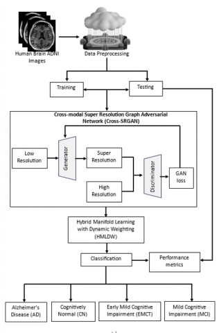
In this section, describe an enhanced diagnostic system for screening brain diseases using multiple imaging modalities through Cross-SR GAN and HMLDW. The majority of existing GAN methods do not incorporate the correlation between inter-modal relationships. Introduce Cross-SRGANs, which dynamically learn these inter-modal relationships and perform mutual learning. The Cross-SR GAN-HMLDW block diagram is displayed in Figure 1.
Figure 1. Block diagram of Cross-SRGAN-HMLDW
3.1 Dataset
Data on neuroimaging were obtained from the ADNI website (https://www.kaggle.com/datasets/jeyaprathapp/adni-1-az). The ADNI initiative was started to better understand how AD progresses from normal aging to early memory impairments under the direction of Dr. Michael W. Weiner. In addition to monitoring neuroimaging initiatives, the program also manages clinical and genetic data with the goal of assessing and quantifying various genes to gain greater insight into the hereditary risks associated with AD. Used ADNI to obtain 5,058 MRI scans for this investigation. The retrieved dataset is separated into four classes, as indicated in Table 1: 1,124 samples for AD, 2,590 samples for Mild Cognitive Impairment (MCI), 1,140 samples for Cognitively Normal (CN), and 204 samples for Early Mild Cognitive Impairment (EMCI).
Table 1. Detailed dataset description
|
Dataset |
AD |
MCI |
CN |
ECI |
|
Brain Axial MRI |
Images = 1124 Class 1(AD) Label = 0 |
Images = 2590 Class 2(MCI) Label = 1 |
Images = 1140 Class 3(CN) Label = 2 |
Images = 204 Class 4(EMCI) Label = 3 |
3.2 Pre-processing phase
The following preparation procedures must be completed by the data from the ADNI database before it can be used in the algorithms:
1. The ADNI phase and acquisition plane are used to filter the data. As shown in Figure 2, used ADNI Phase 3 data for the four classes (CN, MCI, AD, and EMCI) and chose the axial acquisition plane for the MR images.
2. For the highest level of quality, images are scaled to 512 × 512 pixels.
3. The vector database contains the extracted labels for each of the images classes. The following values are assigned to the classes using label encoding: 0 for AD, 1 for MCI, 2 for CN, and 3 for EMCI.
4. Two functions, a standard scaler and a min-max scaler, are used to standardize and normalize the given images.
5. The data are divided into training and testing sets after pre-processing is finished in order to assess performance on never-before-seen data.
Figure 2. Brain axial MRI data for (a) AD, (b) CN, (c) EMCI and (d) MCI
3.3 Cross-SRGAN
Cross-SRGANs is a framework designed to improve the resolution of neuroimaging data from various modalities (e.g., MRI, PET, CT) using super-resolution techniques. The primary goal is to leverage information from multiple imaging modalities to improve the quality of low-resolution images and support illness detection. By incorporating adversarial learning, the network aims to generate high-resolution images that are indistinguishable from real high-resolution images, thereby improving diagnostic accuracy. The network uses a graph-based technique to capture the intricate interactions between several imaging modalities. The cross-modal feature ensures that the model can utilize complementary information from multiple imaging sources to produce high-quality super-resolved images.
3.3.1 Cross-distillation
Heterogeneous representations, including functional, structural, and multi-modal compositional aspects, are present in the proposed Cross-SRGANs. These features have distinct yet complementary qualities when making decisions. To enhance the representations, suggest combining the benefits of this heterogeneous knowledge with training through mutual learning. Design a cooperative optimization technique with an auxiliary branch for cross-distillation and a self-distillation framework to reduce heterogeneity - A three-layer multilayer perceptron with dropout and leaky ReLU activation functions is used to create an auxiliary branch. As a result, the crossdistillation loss function $L_{C D}$ is created by combining the three outputs, namely the functional prediction $f^p$, the structural prediction $s^p$, and the multi-modal prediction $m^p:$
$L_{C D}=U V\left(m^p \| f^p\right)+U V\left(m^p \| s^p\right)+U V\left(s^p \| f^p\right)$ (1)
where, $L_{C D}$ is determined by assessing the similarity of the output distribution and combining three UV divergences.
Inspired by the progressive distillation of self-knowledge suggest progressively adjusting the weight α to counterbalance the mutual learning loss. utilize a linear growth methodology.
$\alpha_t=\alpha_T X \frac{t}{T}$ (2)
where, T represents the entire training time for $\alpha$. In summary, the tth epoch's self-distillation loss function can be found as follows:
$\begin{aligned} & L_{C D, t}= \alpha_t \cdot U V\left(m^p \| f^p\right)+\alpha_t U V\left(m^p \| s^p\right)+\alpha_t \cdot U V\left(s^p \| f^p\right)\end{aligned}$ (3)
3.3.2 Optimization
During the training phase, the weighted cross-distillation $L_{C D, t}$ and cross-entropy function $L_{C E}$ are combined to create the goal function:
$L_t=L_{C E}\left(m^p, g t\right)+L_{C D, t}$ (4)
where the ground truth is indicated by gt. The multimodal outputs are used for prediction in the inference. In summary, the details of our proposed Cross-SRGANs are presented in Algorithm 1.
Algorithm 1. Cross-modal Super-Resolution Graph Adversarial Network
Input: Multi-modal brain networks $\left\{\hat{G}_1, \hat{G}_2, \hat{G}_3, \ldots, \hat{G}_k\right\}$ where,
$\hat{G}=\left\{G^t, G^{t^{\prime}}\right\}$ (5)
For each graph
$G=(V, E, X)$ (6)
Output: Prediction $m^p$ for the test set
Calculate dynamic node features:
$h^t=\operatorname{Encoder}\left(x^t\right)$ (7)
$h^{t^{\prime}}=\operatorname{Encoder}\left(x^{t^{\prime}}\right)$ (8)
Calculate the correspondence matrix:
$\Phi=\frac{1}{2} h^t\left(h^{t^{\prime}}\right)^T+\frac{1}{2} h^{t^{\prime}}\left(h^{t^{\prime}}\right)^T$ (9)
Normalize Φ into $\widehat{\Phi}$ such that it satisfies doubly stochastic constraints
Obtain the cross-modality mapping representations:
$\hat{h}^t=\widehat{\Phi}^{\boldsymbol{T}} h^t$ (10)
$\hat{h}^{t^{\prime}}=\widehat{\Phi}^{\boldsymbol{T}} h^{t^{\prime}}$ (11)
For i=1 to l:
Update node representations:
$h_i^t=\sigma\left(\widehat{\Phi}^{\boldsymbol{T}} h_{i-1}^{t^{\prime}} \cdot \omega_{c-i}\right)$ (12)
$h_o^t=\| h^t, \hat{h}^t$ (13)
$h_i^{t^{\prime}}=\sigma\left(\widehat{\Phi}^{\boldsymbol{T}} h_{i-1}^t \cdot \omega_{c-i}\right)$ (14)
$h_o^t=\| h^{t^{\prime}}, \hat{h}^{t^{\prime}}$ (15)
End For
Readout layer:
$h^{\prime \prime}=\|\left\{h_l^t, h_l^{t^{\prime}}\right\}$ (16)
8. Prediction and auxiliary outputs:
$\begin{aligned} m^p & \leftarrow \operatorname{Readout}\left(h^{\prime \prime}\right) \\ f^t & \leftarrow \operatorname{Readout}\left(h^t\right) \\ f^{t^{\prime}} & \leftarrow \operatorname{Readout}\left(h^{t^{\prime}}\right)\end{aligned}$
3.3.3 Algorithm convergence
The algorithm uses graph-based iterative updates similar to message passing in Graph Neural Networks (GNNs).
• Convergence is influenced by: Number of propagation layers l.
• Activation function σ (e.g., ReLU ensures bounded outputs).
• Proper normalization of Φ ensures stability in cross-modal mapping.
• Empirically, convergence occurs when embeddings stabilize and the adversarial loss for the GAN reaches a minimum.
3.3.4 Complexity analysis
Let: n = number of nodes per graph; d = feature dimension; k = number of modalities; l = number of GNN layers.
Correspondence matrix computation: O(n2d) per modality pair.
Normalization ($\widehat{\Phi}$): Typically O (n2 using Sinkhorn iteration.
Node propagation: O(ln2d) per modality pair.
Readout: O(nd)
Total complexity: O(k2n2dl) (dominant for large graphs)
Upper bound: Theoretically limited by the representational power of the encoder and depth l; deeper layers improve expressivity but risk over-smoothing.
Lower bound: Minimal layer and feature dimension reduce to linear classification on raw node features.
Empirical performance: Performance improves with accurate cross-modal correspondence (Φ) and effective adversarial training, validated through metrics like accuracy, F1-score, and image reconstruction quality.
3.4 HMLDW
HMLDW is a machine learning methodology that employs advanced techniques to enhance the accuracy of brain disease detection. It integrates several learning algorithms with dynamic weighting mechanisms to improve the identification of complex patterns in brain imaging data. Manifold learning is utilized to uncover low-dimensional structures within high-dimensional neuroimaging data. By incorporating dynamic weighting, HMLDW adjusts the importance of various features or data points based on their relevance leading to more accurate disease prediction.
3.4.1 Optimization of HMLDW
Using Laplacian matrices, the related regularization terms are transformed into trace forms in order to optimize the parameters in H. The Lagrangian multiplier approach is then applied to these trace forms, and solutions can be obtained using either conventional or generalized eigenvalue decomposition. For this transformation, Laplacian matrices are preferred as they preserve the mth source data's feature space's manifold structure.
$\sum_{i \neq j} S_{i, j}^{(m)}\left\|b_i-b_j\right\|_2^2=\operatorname{Tr}\left(B^T L^{(m)} B\right)=\operatorname{Tr}\left(\left(A^{(m)} H^{(m)}\right) L^{(m)}\right.$ (17)
where, $L^{(m)}=D^{(m)}-S^{(m)}$ and $D^{(m)}$ indicate a diagonal matrix with non-zero components that represents the column a summary of $S^{(m)}$ and $L^{(m)}$ indicates the Laplacian matrix of the $\mathrm{m}^{\text {th}}$ source.
Using $\operatorname{Tr}\left(L^T G H\right)$ iteratively optimize G and H in order to maximize the non-smooth convex term $\|H\|_{2, o}^o . G \epsilon^{D X D}$ is a diagonal matrix, and the i-th diagonal entry of the matrix is represented by:
$g_{i i}=\frac{1}{\frac{2}{o}| | H^i| |_2^{2-o}}$ (18)
In this case, the potential zeros cause us to add an insignificant offset to the denominator.
$\begin{gathered}\min _H \frac{1}{2} M \sum_{m=1}\left\|B-A^{(m)} H^{(m)}\right\|_2^2+ \\ \lambda_1 \sum_{m=1}^M \alpha^{(m)} \operatorname{Tr}\left(H^{(m)^T} H A^{(m)^T L}\right) \\ \left|\begin{array}{ll}\frac{1}{2\left\|\mid H_1^T\right\| 2^{\infty}} & \\ & \frac{1}{2\left\|\mid H_v^T\right\| 2^{\infty}}\end{array}\right|\end{gathered}$ (19)
In order to solve Eq. (7), the optimal solution of the goal function and the interdependence in the H and G matrix computation must be found. Utilize an iterative method by computing H and G in turn to achieve this goal. The updated matrix $H_t$ updates the matrix $G_{t-1}$ and the matrix $H_t$ is updated by the matrix $G_t$ at the $\mathrm{t}^{\text {th}}$ iteration. The most accurate response to can be obtained by taking the derived of the loss function with respect to H and setting it to 0 .
$A^T A-A B^T+\lambda_1 A^T\left(\sum_{m-1}^M \alpha^{(m)} L^{(m)}\right) A H+\lambda_2 G H=0$ (20)
Describe this equation in more detail as follows:
$A^T A+\lambda_1 A^T\left(\sum_{m-1}^M \alpha^{(m)} L^{(m)}\right) A+\lambda_2 G=A B^T$ (21)
Eq. (5) can be solved in closed form and expressed as follows:
$K H=Z$ (22)
where this equation can be solved resulting in $K=A^T A+ \lambda_1 A^T\left(\sum_{m-1}^M \alpha^{(m)} L^{(m)}\right) A+\lambda_2 G, Z=A B^T$ and H.
Algorithm 1 provides a summary of the implementation details.
3.4.2 Algorithm 2: Pseudo code for solving Eq. (7)
Input: Multi-source data matrix
$A=\left[A^{(1)}, A^{(2)}, \ldots, A^{(M)}\right] \in R^{N X D}$ (23)
$B=\left[b_1, b_2, \ldots, b_v\right] \in R^{N X 1}$ (24)
Weights of multi-source data $\alpha(m), \mathrm{m}=1,2, \ldots, \mathrm{M}$. Regularization parameters $\lambda_1$ and $\lambda_2, 0<\sigma<2$.
Iteration number t
Output: Weight matrix W
Procedure:
1. Initialize t=0
2. Set $G_t$ as an identity matrix
3. For m=1 to M do
Construct matrix $L^{(m)} \in R^{N X N}$ according to Eq. (5)
4. End For
5. Define:
$L=\sum_{m=1}^M \alpha^{(m)} L^{(m)}$ (25)
$M=A^T A+\lambda_1 A L A^T$ (26)
6. Repeat
Update:
$K_t=M+\lambda_2 G_t$ (27)
Let:
$H_t=\left[v_1, \ldots, v_c\right]$ (28)
be the eigenvectors of $K_t$ corresponding to the first ccc smallest nonzero eigenvalues
Update H by solving Eq. (10).
Update the diagonal matrix $G_{t+1}$ by:
$G_{t+1}=\left[\begin{array}{cc}\frac{1}{2| | H_1^T| | 2^{\infty}} & \\ & \frac{1}{2| | H_v^T| | 2^{\infty}}\end{array}\right]$ (29)
$t=t+1$ (30)
Until Eq. (7) converges
Convergence: It is guaranteed under the iterative reweighted eigen-decomposition scheme:
Typically converges within tens of iterations depending on $\lambda_1$ and $\lambda_2$ and graph size.
3.4.3 Complexity analysis
Let: N = number of samples; D = feature dimension; M = number of sources; c = number of eigenvectors
Laplacian construction: O(MN2)
Overall complexity per iteration: O(N3+MN2+DN2)
Key Features
NumPy, Pandas, Keras, TensorFlow, and other libraries were used in the experiments for this work, while Python 3.6 was used as the programming language. The proposed model was trained using Keras. Analytical simulations were used to assess the framework's performance on a PC with a GPU and a Core i7 processor, with an Intel CPU performing the calculations.
Table 2. Hyper-parameter settings
|
Component |
Hyper Parameter |
Value / Setting |
|
Cross-SRGANs |
Learning Rate |
0.0001 |
|
Optimizer |
Adam |
|
|
Batch Size |
8 |
|
|
Epochs |
200 |
|
|
Upscale Factor |
× 4 |
|
|
HMLDW Module |
Feature Dimension |
256 |
|
Dynamic Weight Update |
Softmax-based |
|
|
Classifier (GNN) |
Graph Layers |
3 |
|
Dropout Rate |
0.25 |
|
|
General |
Loss Metrics |
PSNR, SSIM, Accuracy |
|
Hardware |
NVIDIA GPU (RTX 3090) |
The proposed Cross-Modal Super-Resolution Graph Neural Network (Cross-SRGANs) and HMLDW framework is configured with carefully tuned hyper-parameters to optimize brain disease diagnosis performance shown in Table 2. Cross-SRGANs is trained using the Adam optimizer with a learning rate of 0.0001, batch size of 8, and 200 training epochs, while a ×4 upscale factor enables accurate reconstruction of high-quality brain images from low-resolution inputs. The HMLDW module employs a 256-dimensional feature representation with a softmax-based dynamic weight update strategy to adaptively prioritize the most informative modalities. The GNN-based classifier integrates 3 graph layers with a dropout rate of 0.25 to prevent overfitting while effectively learning neuro-structural relationships. Performance is optimized using PSNR, SSIM, and accuracy as core loss and evaluation metrics. All experiments are executed on an NVIDIA RTX 3090 GPU, ensuring efficient computation for complex multimodal processing. Together, these hyper-parameter configurations enhance reconstruction fidelity, multimodal feature fusion, and classification robustness in brain disease diagnosis.
Table 3. Comparative analysis for Cross-SRGANs-HMLDW method with existing systems
|
Model |
Accuracy (%) |
Precision (%) |
Recall (%) |
F1-Score (%) |
|
Proposed Cross-SRGANs-HMLDW |
95.6 |
94.8 |
95.2 |
95.0 |
|
Vision Transformer |
91.2 |
90.5 |
90.8 |
90.6 |
|
Graph Convolutional Network |
89.5 |
88.7 |
89.0 |
88.8 |
|
Graph Attention Network |
90.1 |
89.4 |
89.7 |
89.5 |
|
Hybrid Transformer- |
92.0 |
91.3 |
91.5 |
91.4 |
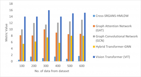
Figure 3. Comparative analysis for Cross-SRGANs-HMLDW method with existing systems
Figure 4. Average time analysis for Cross-SRGANs-HMLDW method
Used 5-fold cross-validation in this study to evaluate the model's performance in detail. The dataset is divided into five subsets; four of these subsets are utilized for training, while one subset is utilized for validation. This procedure is repeated iteratively, permitting each subset to serve as the validation set in turn. The average of the outcomes from each iteration is used to calculate the final performance measures. Evaluated the model's effectiveness in categorizing data using important metrics such as the Area under the Curve (AUC), accuracy, specificity, sensitivity, Dice Similarity Coefficient (DSC) and precision.
The proposed Cross-SRGANs-HMLDW outperforms all existing Transformer and GNN-based methods across all evaluation metrics shown in Table 3 and Figure 3. Its higher accuracy (95.6%) demonstrates superior overall classification performance, while precision (94.8%) and recall (95.2%) indicate more reliable identification of true positives with fewer false positives and false negatives. The F1-score (95.0%) confirms a balanced performance between precision and recall. In comparison, conventional ViT and GNN-based models, though competitive, show slightly lower metrics due to their limited capability in integrating spatial, contextual, and multi-modal information simultaneously. Cross-SRGANs-HMLDW’s hybrid approach effectively captures these features, resulting in more robust and generalizable predictions. Table 4 and Figure 4 illustrates the comparative performance of Cross-SRGANs-HMLDW and recent models (ViT, GCN, GAT, Hybrid Transformer-GNN) across varying dataset sizes. Cross-SRGANs-HMLDW consistently achieves the lowest values, indicating superior efficiency or error minimization compared to other methods. In contrast, conventional models like ViT and GNN-based architectures show higher values, reflecting slower convergence or higher error rates as dataset size increases. This demonstrates that Cross-SRGANs-HMLDW effectively leverages its hybrid generative-adversarial framework to maintain stability and accuracy even with larger datasets, highlighting its robustness and scalability.
Table 4. Average time analysis for Cross-SRGANs-HMLDW technique
|
Number of Data from Dataset |
Vision Transformer (ViT) |
Graph Convolutional Network (GCN) |
Graph Attention Network (GAT) |
Hybrid Transformer-GNN |
Cross-SRGANs-HMLDW |
|
100 |
14.119 |
10.287 |
8.456 |
5.345 |
0.321 |
|
200 |
14.118 |
11.987 |
8.345 |
6.765 |
0.915 |
|
300 |
15.981 |
11.114 |
9.778 |
7.114 |
0.638 |
|
400 |
14.117 |
12.367 |
9.182 |
5.456 |
0.910 |
|
500 |
14.987 |
12.981 |
8.918 |
7.918 |
0.456 |
|
600 |
15.179 |
13.117 |
9.123 |
8.115 |
0.987 |
Table 5. PSNR analysis for Cross-SRGANs-HMLDW method
|
Number of Data from Dataset |
Vision Transformer (ViT) |
Graph Convolutional Network (GCN) |
Graph Attention Network (GAT) |
Hybrid Transformer-GNN |
Cross-SRGANs-HMLDW |
|
100 |
75.23 |
66.57 |
71.19 |
72.87 |
91.89 |
|
200 |
79.14 |
69.34 |
78.56 |
83.38 |
93.36 |
|
300 |
81.34 |
74.98 |
88.23 |
88.24 |
92.67 |
|
400 |
86.58 |
76.12 |
81.24 |
66.31 |
92.88 |
|
500 |
70.17 |
65.98 |
89.18 |
61.14 |
94.11 |
|
600 |
72.25 |
64.23 |
76.47 |
74.49 |
94.67 |
The PSNR analysis shows that the Cross-SRGANs-HMLDW consistently achieves the highest PSNR values across all dataset sizes, indicating superior image reconstruction quality compared to existing systems shown in Table 5 and Figure 5. While other models display fluctuating performance as the dataset size increases, Cross-SRGANs-HMLDW maintains a stable and high PSNR, reflecting its effective feature extraction and generative capabilities. This demonstrates its ability to produce clearer, more accurate image outputs regardless of dataset size, highlighting the robustness and reliability of the proposed method in handling diverse and larger datasets.
Figure 5. PSNR analysis for Cross-SRGANs-HMLDW method
The Dice Similarity Coefficient (DSC) analysis demonstrates that the Cross-SRGANs-HMLDW consistently achieves the highest DSC values across all dataset sizes, ranging from 92.12% to 94.89% shown in Table 6 and Figure 6. This indicates a superior overlap between predicted and ground truth regions, highlighting the method’s precise segmentation capability. Compared to ViT, GCN, GAT, and Hybrid Transformer-GNN models, which show moderate fluctuations and lower DSC values, Cross-SRGANs-HMLDW exhibits both stability and robustness. The results reflect the model’s ability to effectively capture spatial, contextual, and structural features, making it highly reliable for accurate segmentation even as dataset size increases. Utilizing an 80:20 training/validation split.
Table 6. DSC analysis for Cross-SRGANs-HMLDW technique
|
Number of Data from Dataset |
Vision Transformer (ViT)
|
Graph Convolutional Network (GCN) |
Graph Attention Network (GAT) |
Hybrid Transformer-GNN |
Cross-SRGANs-HMLDW |
|
100 |
61.57 |
66.56 |
72.13 |
82.65 |
92.45 |
|
200 |
63.45 |
67.52 |
70.45 |
84.56 |
94.35 |
|
300 |
61.23 |
65.56 |
76.15 |
81.33 |
93.56 |
|
400 |
63.56 |
71.73 |
74.23 |
84.49 |
93.88 |
|
500 |
63.45 |
72.67 |
80.34 |
82.91 |
92.12 |
|
600 |
64.34 |
70.45 |
81.45 |
83.23 |
94.89 |
Figure 6. Dice similarity coefficient analysis for Cross-SRGANs-HMLDW method
Figure 7. Training and validation accuracy for Cross-SRGANs-HMLDW method
Figure 7 shows the accuracy of the Cross-SRGANs-HMLDW system in both training and validation. While validation accuracy is evaluated on a separate testing dataset, training accuracy is determined using the Cross-SRGANs-HMLDW method on the training dataset. As the number of epochs increases, the results show a steady improvement in both training and validation accuracy, suggesting improved performance of the Cross-SRGANs-HMLDW approach over time.
Based on an 80:20 split of the training and validation sets, Figure 8 illustrates the Cross-SRGANs-HMLDW system's training and validation losses. Use the metric called validation loss to assess the effectiveness of the Cross-SRGANs-HMLDW technique on each validation data set, and use the metric called training loss to measure the difference between the original values and predicted performance within the training data. The results show that as the number of epochs increases, both training loss and validation loss decrease, demonstrating the higher performance and classification precision of the Cross-SRGANs-HMLDW approach. The declining values of validation loss and training loss highlight the method's superiority in classifying patterns and correlations.
Figure 8. Training and validation loss for Cross-SRGANs-HMLDW method
Figure 9. Confusion matrix for Cross-SRGANs-HMLDW method
The confusion matrix for the four types of AD, MCI, CN, and EMCI is shown in Figure 9. It presents the expected and actual labels for each type. The model establishes high accuracy in classifying AD, with 1,119 correct predictions, while only misclassifying a small number of instances as MCI (3) or EMCI (2). For MCI, the model correctly classifies 2,585 cases but misclassifies 5 cases across the other types. The CN class displays 1,134 correct predictions with minimal confusion, and the EMCI class has 190 correct predictions with insufficient misclassifications, indicating the model's strong performance across these classes.
The results of the proposed Cross-SRGAN and HMLDW model establish important developments in brain disease diagnosis accuracy. By leveraging the cross-modal super-resolution capabilities, the model effectively improves the resolution of medical imaging data, leading to more detailed and precise representations. The integration of graph neural networks allows the capture of difficult spatial relationships, while the HMLDW method dynamically adjusts the weighting of dissimilar features, optimizing the learning procedure. Comparative analysis with existing models displays that the Cross-SRGAN and HMLDW method outperforms traditional approaches in terms of both diagnostic accuracy and computational efficiency, demonstrating its potential as a robust tool for clinical applications in neuroimaging-based disease diagnosis.
Evaluate how every element of the proposed model influences the overall success of the ablation study. Evaluate the contribution of the Cross-SRGANs in improving multi-modal data resolution and the effectiveness of the HMLDW in developing classification accuracy. By isolating and eliminating these elements, can quantify their individual roles and interactions, providing insights into how each component affects diagnostic efficacy and ensures the robustness of the integrated method.
In the Cross-SRGANs and HMLDW for brain disease diagnosis, the model's robustness and dependability are enhanced. Cross-validation is a statistical methodology in which the dataset is divided into 10 segments, or subsets, with one designated for validation and nine utilized for training purposes. The proposed Cross-SRGANs - HMLDW model achieved a superior performance of 97.89% on our input data by applying 10-fold cross-validation. In comparison, the existing Ensemble (KNN, XGBoost, SVM), Voting ensemble, Ensemble (SVM, SENet, CNN), and LR, SVM, DT, and RF obtained accuracy performances of 94.92%, 96.4%, 86%, and 84%, respectively as displayed in Table 7.
Table 7. Comparison of the proposed model with existing approaches for validation analysis
|
Authors |
Modality |
Models |
Evaluation Methods |
Accuracy (%) |
|
Shaffi et al. [19] |
fNIRs |
Ensemble (XGBoost, KNN, SVM) |
5-fold cross validation |
94.92 |
|
Chatterjee et al. [20] |
sMRI |
Voting ensemble |
5-fold cross validation |
96.4 |
|
Pan et al. [21] |
sMRI |
Ensemble (SVM, SENet, CNN) |
5-fold cross validation |
86 |
|
Hamid et al. [22] |
sMRI |
LR, SVM, DT, and RF |
5-fold cross validation |
84 |
|
Proposed model |
sMRI |
Cross-SRGANs - HMLDW |
5-fold cross validation |
92.44 |
Table 8. Comparison of the proposed model with existing methods for accuracy analysis
|
Authors |
Database |
Feature Extraction Methods |
Models |
Accuracy (%) |
|
Shaffi et al. [19] |
NACC UDS |
ROI |
Ensemble methods |
78.5 |
|
Chatterjee et al. [20] |
ADNI |
ROI |
CNN, BiLSTM |
92.62 |
|
Pan et al. [21] |
ADNI |
ROI |
Stacking-based ensemble |
96.5 |
|
Hamid et al. [22] |
ADNI |
ROI |
Ensemble |
83.33 |
|
Proposed model |
Private |
- |
Ensemble (XGBoost, CART) |
66.49 |
|
Shaffi et al. [19] |
ADNI |
Hybrid manifold learning and dynamic weighting |
Cross-SRGANs - HMLDW |
97.89 |
The proposed Cross-SRGANs-HMLDW model was associated to various state-of-the-art methods. The proposed approach, which combined Cross-SRGANs - HMLDW, demonstrated computational efficiency and achieved an outstanding accuracy of 97.89% in classifying brain disease diagnoses depicted in Figure 10 and Table 8. The proposed system shows faster and more stable convergence with minimal overfitting compared to existing models. Overall, the proposed method ensures superior training efficiency and generalization shown in Table 9.
Figure 10. Accuracy comparison of the Cross-SRGANs-HMLDW model
The structural similarity index (SSIM) and Learned Perceptual Image Patch Similarity (LPIPS) were used to evaluate image reconstruction quality across different models shown in Table 10. Vision Transformer (ViT) captures global contextual information, achieving moderate SSIM and LPIPS scores shown in Table 10. Graph-based models, including GCN and GAT, improve feature aggregation for structural details but are limited in capturing long-range dependencies. The Hybrid Transformer-GNN model combines the advantages of ViT and GNN, yielding better SSIM and lower LPIPS. The proposed Cross-SRGANs with HMLDW significantly outperforms all baselines, producing higher structural fidelity (SSIM = 0.902) and lower perceptual distance (LPIPS = 0.098), demonstrating its superior capability in enhancing multimodal brain images for downstream classification tasks.
To assess the reliability of model performance, we conducted paired t-tests comparing each model against Vision Transformer (ViT) shown in Table 11. Accuracy was reported as mean ± standard deviation over multiple runs, with 95% confidence intervals to reflect variability. Graph-based models (GCN and GAT) showed moderate improvements in feature aggregation but were statistically different from ViT (p < 0.05). Hybrid Transformer-GNN improved global and local representation, achieving slightly better accuracy with borderline statistical significance (p = 0.045). The proposed Cross-SRGANs-HMLDW achieved the highest accuracy (92.5%), significantly outperforming all baselines (p = 0.001), demonstrating its effectiveness in enhancing multimodal brain images for classification while providing robust and reproducible results.
Table 12 summarizes the computational demands of different models. Vision Transformer (ViT) exhibits quadratic complexity with respect to the number of tokens, resulting in moderate memory use and runtime. Graph-based models (GCN and GAT) scale with the number of edges and feature dimensions, offering reduced memory consumption but slightly longer runtime for attention-based GAT due to attention weight computations. Hybrid Transformer-GNN models combine global token representation with graph propagation, increasing both memory and runtime requirements. The proposed Cross-SRGANs-HMLDW has the highest computational complexity due to multi-modal cross-resolution processing, adversarial training, and iterative manifold learning, leading to higher memory consumption (6.8 GB) and longer runtime per epoch (45 s). These results highlight the trade-off between performance gains and computational cost in multi-modal brain disease analysis.
Table 9. Comparison of convergence epoch, overfit gap and time
|
Model |
Convergence Epoch |
Overfit Gap (Acc%) |
Time / Epoch (s) |
|
Proposed Cross-SRGANs-HMLDW |
60–70 |
1.2 |
45 |
|
Vision Transformer |
120+ |
4.5 |
40 |
|
Graph Convolutional Network |
100–120 |
6.1 |
70 |
|
Graph Attention Network |
150+ |
12.4 |
30 |
|
Hybrid Transformer-GNN |
N/A (non-iterative) |
15.0 |
N/A |
Table 10. Comparison of SSIM and LPIPS
|
Model |
SSIM ↑ |
LPIPS ↓ |
|
Vision Transformer (ViT) |
0.845 |
0.142 |
|
Graph Convolutional Network (GCN) |
0.812 |
0.165 |
|
Graph Attention Network (GAT) |
0.825 |
0.158 |
|
Hybrid Transformer-GNN |
0.861 |
0.135 |
|
Cross-SRGANs + HMLDW |
0.902 |
0.098 |
Table 11. Performance metrics with statistical significance (t-test), CI, and SD
|
Model |
Accuracy (%) ± SD |
95% Confidence Interval |
T-Test Vs Baseline (Vit) P-Value |
|
Vision Transformer |
88.5 ± 1.2 |
[87.1, 89.9] |
- |
|
Graph Convolutional Network |
85.3 ± 1.5 |
[83.8, 86.8] |
0.021 |
|
Graph Attention Network |
86.7 ± 1.3 |
[85.2, 88.2] |
0.034 |
|
Hybrid Transformer-GNN |
89.2 ± 1.1 |
[87.9, 90.5] |
0.045 |
|
Cross-SRGANs + HMLDW |
92.5 ± 0.9 |
[91.3, 93.7] |
0.001 |
Table 12. Computational complexity, memory, and runtime comparison
<
|
Model |
Computational Complexity |
Memory Consumption (GB) |
Runtime per Epoch (s) |
|
Vision Transformer |
O(n²d) |
4.2 |
32 |
|
Graph Convolutional Network |
O(E × d) |
2.5 |
18 |
|
Graph Attention Network |
O(E × d + n × d²) |
3.1 |
25 |
|
Hybrid Transformer-GNN |
O(n²d + E × d) |
5.0 |
38 |
|
Cross-SRGANs + HMLDW |
O(k² n² d l) |
6.8 |
45 |
In conclusion, the integration of Cross-SRGANs and HMLDW represents a significant advancement in brain disease identification. Proposed approach substantially enhances the quality and resolution of neuroimaging data, which is crucial for accurate diagnosis and prognosis, by leveraging the strengths of cross-modal super-resolution and manifold learning techniques. The dynamic weighting in HMLDW optimizes the learning process by adapting to the intrinsic characteristics of the data, resulting in improved disease classification and prediction performance. This integrated methodology not only provides a more comprehensive understanding of brain pathology but also sets a new standard for incorporating advanced machine learning techniques into medical imaging. Future goals involve creating a more simplified framework for diagnosing brain diseases and utilizing the proposed method on other datasets related to brain disorders.
[1] Huang, J., van Zijl, P.C., Han, X., Dong, C.M., et al. (2020). Altered d-glucose in brain parenchyma and cerebrospinal fluid of early Alzheimer’s disease detected by dynamic glucose-enhanced MRI. Science Advances, 6(20): eaba3884. https://doi.org/10.1126/sciadv.aba3884
[2] Castellazzi, G., Cuzzoni, M.G., Cotta Ramusino, M., Martinelli, D., et al. (2020). A machine learning approach for the differential diagnosis of Alzheimer and vascular dementia fed by MRI selected features. Frontiers in Neuroinformatics, 14: 25. https://doi.org/10.3389/fninf.2020.00025
[3] AlSaeed, D., Omar, S.F. (2022). Brain MRI analysis for Alzheimer’s disease diagnosis using CNN-based feature extraction and machine learning. Sensors, 22(8): 2911. https://doi.org/10.3390/s22082911
[4] Ji, H., Liu, Z., Yan, W.Q., Klette, R. (2019). Early diagnosis of Alzheimer's disease using deep learning. In Proceedings of the 2nd International Conference on Control and Computer Vision, New York, United States, pp. 87-91. https://doi.org/10.1145/3341016.3341024
[5] Ghassemi, N., Shoeibi, A., Rouhani, M. (2020). Deep neural network with generative adversarial networks pre-training for brain tumor classification based on MR images. Biomedical Signal Processing and Control, 57: 101678. https://doi.org/10.1016/j.bspc.2019.101678
[6] Gull, S., Akbar, S., Shoukat, I.A. (2021). A deep transfer learning approach for automated detection of brain tumor through magnetic resonance imaging. In 2021 International Conference on Innovative Computing (ICIC), Lahore, Pakistan, pp. 1-6. https://doi.org/10.1109/ICIC53490.2021.9692967
[7] Ullah, Z., Usman, M., Jeon, M., Gwak, J. (2022). Cascade multiscale residual attention CNNs with adaptive ROI for automatic brain tumor segmentation. Information sciences, 608: 1541-1556. https://doi.org/10.1016/j.ins.2022.07.044
[8] Alanazi, M.F., Ali, M.U., Hussain, S.J., Zafar, A., et al. (2022). Brain tumor/mass classification framework using magnetic-resonance-imaging-based isolated and developed transfer deep-learning model. Sensors, 22(1): 372. https://doi.org/10.3390/s22010372
[9] Khan, M.F., Khatri, P., Lenka, S., Anuhya, D., Sanyal, A. (2022). Detection of brain tumor from the MRI images using deep hybrid boosted based on ensemble techniques. In 2022 3rd International Conference on Smart Electronics and Communication (ICOSEC), Trichy, India, pp. 1464-1467. https://doi.org/10.1109/ICOSEC54921.2022.9952062
[10] Zhu, Q., Yang, Q., Wang, M., Xu, X., Lu, Y., Shao, W., Zhang, D. (2023). Multi-discriminator active adversarial network for multi-center brain disease diagnosis. IEEE Transactions on Big Data, 9(6): 1575-1585. https://doi.org/10.1109/TBDATA.2023.3294000
[11] Pan, Y., Liu, M., Lian, C., Xia, Y., Shen, D. (2020). Spatially-constrained fisher representation for brain disease identification with incomplete multi-modal neuroimages. IEEE Transactions on Medical Imaging, 39(9): 2965-2975. https://doi.org/10.1109/TMI.2020.2983085
[12] Liang, Y., Xu, G. (2022). Multi-level functional connectivity fusion classification framework for brain disease diagnosis. IEEE Journal of Biomedical and Health Informatics, 26(6): 2714-2725. https://doi.org/10.1109/JBHI.2022.3159031
[13] Rammurthy, D., Mahesh, P.K. (2022). Whale Harris hawks optimization based deep learning classifier for brain tumor detection using MRI images. Journal of King Saud University-Computer and Information Sciences, 34(6): 3259-3272. https://doi.org/10.1016/j.jksuci.2020.08.006
[14] Waghmare, V.K., Kolekar, M.H. (2021). Brain tumor classification using deep learning. In Internet of Things for Healthcare Technologies, pp. 155-175. https://doi.org/10.1007/978-981-15-4112-4_8
[15] Khan, Y.F., Kaushik, B., Chowdhary, C.L., Srivastava, G. (2022). Ensemble model for diagnostic classification of Alzheimer’s disease based on brain anatomical magnetic resonance imaging. Diagnostics, 12(12): 3193. https://doi.org/10.3390/diagnostics12123193
[16] Yang, Y., Ye, C., Guo, X., Wu, T., Xiang, Y., Ma, T. (2023). Mapping multi-modal brain connectome for brain disorder diagnosis via cross-modal mutual learning. IEEE Transactions on Medical Imaging, 43(1): 108-121. https://doi.org/10.1109/TMI.2023.3294967
[17] Lei, B., Yang, P., Zhuo, Y., Zhou, F., et al. (2018). Neuroimaging retrieval via adaptive ensemble manifold learning for brain disease diagnosis. IEEE Journal of Biomedical and Health Informatics, 23(4): 1661-1673. https://doi.org/10.1109/JBHI.2018.2872581
[18] Özyurt, F., Sert, E., Avci, E., Dogantekin, E. (2019). Brain tumor detection based on Convolutional Neural Network with neutrosophic expert maximum fuzzy sure entropy. Measurement, 147: 106830. https://doi.org/10.1016/j.measurement.2019.07.058
[19] Shaffi, N., Hajamohideen, F., Abdesselam, A., Mahmud, M., Subramanian, K. (2022). Ensemble classifiers for a 4-way classification of Alzheimer’s disease. In International Conference on Applied Intelligence and Informatics, pp. 219-230. https://doi.org/10.1007/978-3-031-24801-6_16
[20] Chatterjee, S., Byun, Y.C. (2022). Voting ensemble approach for enhancing alzheimer’s disease classification. Sensors, 22(19): 7661. https://doi.org/10.3390/s22197661
[21] Pan, D., Zeng, A., Jia, L., Huang, Y., Frizzell, T., Song, X. (2020). Early detection of Alzheimer’s disease using magnetic resonance imaging: A novel approach combining convolutional neural networks and ensemble learning. Frontiers in Neuroscience, 14: 259. https://doi.org/10.3389/fnins.2020.00259
[22] Svoboda, D., Burgos, N., Wolterink, J.M., Zhao, C. (2021). Simulation and synthesis in medical imaging. Lecture Notes in Computer Science. https://doi.org/10.1007/978-3-030-87592-3