Hatice Tombul Çalışkan*![]() | Hacer Karacan
| Hacer Karacan![]()
© 2025 The authors. This article is published by IIETA and is licensed under the CC BY 4.0 license (http://creativecommons.org/licenses/by/4.0/).
OPEN ACCESS
Defense needs of countries are increasing due to developing technologies. RADAR and SONAR systems used in military and civil applications are effective for detecting objects in specific areas. These systems broadcast radio or sound waves at various frequencies and wavelengths and determine object positions and sizes from reflected signals. However, such diffusion reveals the source’s location, especially in military use, making it a target for guided munitions with passive radar. In contrast, locating subsonic objects via Sound Source Localization (SSL) enables their detection without becoming the target, offering strategic defense value. This paper introduces a novel method based on geometric analysis for estimating the position of a stationary sound source. Artificial Neural Networks (ANNs) were employed to benchmark the performance of the proposed localization approach. Both the proposed method and the ANN model were evaluated using experimental data collected in an indoor environment. The experiments were conducted in a realistic domestic acoustic environment, where acoustic signals were recorded using three electret microphones and a National Instruments data acquisition system. The performance of both methods was assessed using multiple evaluation metrics. Experimental results demonstrate that the proposed approach outperforms the ANN model, offering a more accurate and reliable solution for SSL.
acoustic source localization, loop closure equation, microphone array, time delay estimation, vector loops
In modern societies, a wide range of devices, materials, and equipment constantly produce sounds that are perceived through pressure variations in the ear. The human brain has an extraordinary capacity to identify and locate these sound sources, a process referred to as sound localization in neuroscience. Inspired by this natural ability, researchers have long sought to replicate it in artificial systems. The task of determining the position of an acoustic source using microphones is widely known as Sound Source Localization (SSL).
With the continuous advancement of technology, national defense requirements have grown increasingly complex. Traditional detection systems such as RADAR and SONAR have long been employed in both military and civilian applications to identify objects within a specific area. These systems operate by transmitting radio or sound waves at various frequencies and wavelengths, then estimating an object’s position and size from the reflected signals. While highly effective, this active emission approach has a critical drawback in military contexts: it exposes the emitter’s location, making it vulnerable to passive detection and precision-guided attacks. In contrast, SSL offers a passive alternative, capable of tracking objects moving at subsonic speeds without revealing the observer’s position. This makes SSL a promising technology for advancing defense systems and enhancing national security. Beyond defense, SSL has also attracted substantial attention due to its broad range of applications, including hearing aids, robotics, navigation, speaker tracking, remote sensing, and security-related systems such as surveillance, gunshot detection, and artillery localization.
Most existing SSL studies have relied on professional grade large microphone arrays (e.g., 4–56 Brüel & Kjær or Eigenmike microphones). These studies were typically conducted in acoustically controlled environments such as anechoic or semi-anechoic chambers [1-5]. While these studies have advanced SSL, their reliance on expensive hardware and ideal conditions limits their applicability in everyday environments. Additionally, there is a lack of research on low-cost and simple setups with only a few nonlinearly placed microphones in real-world environments, characterized by naturally occurring noise and reverberation which cause performance degradation in most existing systems. Despite significant progress in SSL, recent surveys highlight, challenges persist, including artificial intelligence-based models' heavy reliance on training data and the difficulty of achieving reliable and robust localization in realistic, dynamic acoustic environments [6, 7]. Therefore, there is a critical gap between the controlled, professional grade setups dominating the literature and the need for cost-effective, robust SSL methods that function reliably in everyday environments. This study directly addresses this gap by introducing a low-cost, practical SSL approach and validating it in realistic domestic conditions.
Our contribution is twofold: first, we propose a new SSL method that can be implemented with three low-cost MAX9814 microphones and a National Instruments (NI) USB-6216 interface; second, we provide a direct comparison of the proposed method and an Artificial Neural Network (ANN) model using our own data recorded in realistic domestic environments. The economic advantage of our approach is significant. At the component level, the cost of our three microphones is orders of magnitude lower than that of a single microphone module in professional arrays such as Eigenmike or Brüel & Kjær systems. While we used an NI USB-6216 interface in this study for its proven reliability and performance, our localization method is algorithmically independent of this specific hardware. This means that for applications where budget is the primary constraint, the method can work with lower-cost data acquisition solutions, potentially reducing the total system cost further compared to our current setup. Overall, the total cost of our reference setup remains more than an order of magnitude lower than that of professional systems. The use of inexpensive, widely available microphones highlights the feasibility of the method for practical, low-budget implementations. By combining methodological novelty with clear economic advantages, this study demonstrates a practical and cost-effective approach to SSL that can benefit real-world applications requiring both accuracy and affordability.
The structure of this paper is as follows: Section 2 provides a brief literature review of similar studies on SSL. Section 3 is divided into subsections explaining the experimental setup and acoustic characterization, data preparation, the proposed method, and the ANN used for performance comparison. The obtained results are presented, thoroughly compared, and discussed in detail in Section 4. Section 5 addresses the study's limitations and suggests future work. Finally, Section 6 concludes the paper by summarizing the key findings and outlining opportunities for future research.
Numerous theoretical and experimental studies have explored various microphone array geometries and configurations for SSL. Microphones are fundamental components of SSL systems, and both their arrangement and number critically affect localization accuracy. Since SSL relies on analyzing signal variations across sensors, at least two microphones are typically required, although single-microphone approaches have also been reported [8-10]. Given this fundamental role of array design, many studies have investigated SSL performance under different recording conditions.
Localization in reverberant or noisy environments is particularly challenging, so many studies have been conducted in anechoic or semi-anechoic conditions. These investigations typically have relied on complex setups involving more than three microphones and professional-grade recording equipment. For example, Poschadel et al. [1] used deep learning-based localization with a 32-channel Eigenmike array and motion capture system under ITU-R BS.1116-3 compliant conditions. Jung and Ih [2] designed compact tetrahedral, hexahedral, and octahedral arrays of Brüel & Kjær microphones and tested them in anechoic chambers. Similarly, Padois et al. [3] investigated SSL using a spherical array of Brüel & Kjær microphones in a semi-anechoic chamber, while Ma et al. [4] validated their indoor localization method in a controlled reverberation chamber with 15 Brüel & Kjær microphones. Chen et al. [5] evaluated their hybrid approach in a semi-anechoic chamber using a 56-channel spiral array with 40 actively used Brüel & Kjær microphones.
Several studies have focused on traditional methods. For instance, Flood and Elvanter [11] used Time Difference of Arrival (TDOA) for multiple-source localization, while Xiong et al. [12] extended TDOA to non-line-of-sight scenarios using a neurodynamic solution. Zhang et al. [13] combined TDOA and Frequency Difference of Arrival (FDOA) for underwater applications. Padois et al. [14] and Lee et al. [15] applied generalized cross-correlation techniques, including GCC-PHAT, with spherical and two-microphone arrays. Firoozabadi et al. [16] integrated generalized eigenvalue decomposition with adaptive GCC-PHAT/Maximum Likelihood (ML) in a T-shaped circular array, while Villadangos et al. [17] and Zou and Liu [18] enhanced Time of Arrival (TOA) measurements for ultrasonic and acoustic localization. Subspace-based approaches, such as MUSIC and ESPRIT [19-21], have also been widely used, including ESPRIT combined with Direct Augmentation and Spatial Smoothing for more sources than sensors [20]. Finally, Yang et al. [22] proposed a bat algorithm-based 3D-MUSIC algorithm for fast SSL and it outperformed conventional 3D-MUSIC in semi-anechoic tests.
Beyond these, alternative methods have been developed. Lai et al. [23] developed an advanced Steered Response Power (SRP) method using a 16-microphone planar array in a reverberant room. Feng et al. [24] proposed a framework to eliminate quantization errors in classification-based SSL with circular and linear 4-microphone arrays. Fischer et al. [25] evaluated sparse array geometries, showing open-box arrays perform best, while coprime arrays perform worst. Heydari and Mahabadi [26] demonstrated that multiple parallel distributed arrays improve localization accuracy.
In recent years, artificial intelligence-based models have gained increasing attention. Toma et al. [27] proposed a three stage Convolutional Neural Network (CNN) with a fusion layer for speaker localization with a four-microphone linear array. Similarly, Zhu and Wan [28] developed a GCC-PHAT-based CNN model and validated its performance with simulated data. Tan et al. [29] introduced a hybrid CNN-Regression (CNN-R) model, while Hu et al. [30] presented a residual network with channel attention for localization tasks. Correia et al. [31] designed a deep feedforward neural network for energy-based SSL, evaluating it across scenarios with 3, 6, 9, 12, and 15 microphones arranged in a circle under ideal, noise-free conditions. The network was trained on noise-free data and tested against varying noise levels. Yang et al. [32] proposed a Recurrent Neural Network (RNN) approach for Direction of Arrival (DOA) estimation, achieving lower errors than conventional methods like beamforming and MUSIC. These studies highlight the increasing role of AI in improving the accuracy and robustness of SSL.
Despite these advancements, several limitations remain. Khan et al. [6] reviewed developments, challenges, and applications in SSL and emphasized that achieving accurate and precise localization in complex and dynamic acoustic environments is still a major challenge. Xu et al. [7] highlighted that modern deep learning-based methods fail to demonstrate sufficiently robust performance under noise and reverberation, struggle with real-time requirements, and depend heavily on large training datasets. These findings confirm that while progress has been substantial, the robustness and reliability of SSL techniques in realistic conditions remain limited.
In this study, a novel sound source localization method based on geometric analysis is proposed. The acoustic data were experimentally recorded using three microphones arranged at 120° intervals in a moderately noisy, reverberant indoor environment. The signals captured by the microphone array were saved for analysis, and the performance of the proposed method was evaluated using this dataset. The primary objective of this study is to estimate the position of a stationary sound source based on experimental data using the proposed geometric approach. Additionally, an ANN model was trained using the same dataset, and its performance was compared with that of the proposed method.
In this section, we present in subsections the experimental setup and environmental characterization, data preparation and filtering, proposed method for SSL along with the ANN architecture used to benchmark its performance.
3.1 Experimental setup and acoustic characterization
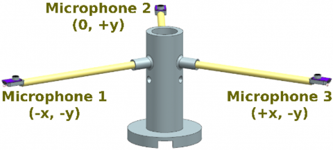
To ensure the validity of the proposed method, both the experimental setup and the acoustic environment were carefully characterized. The experiments were conducted in a real-world indoor environment with echoic and noise-prone conditions, and the acoustic data-hand claps were collected. The setup consisted of three electret microphones, each equipped with a MAX9814 microphone amplifier, positioned at an angle of 120 degrees to each other and placed at an arm length of 50 cm. MAX9814 is a microphone amplifier with 3 adjustment options for gain and AR (attack/release) pins and is built on automatic gain control. The center of the gray platform, shown in Figure 1, was defined as the point (0, 0). The positions of the microphones were determined in meters as (-0.25√3, -0.25), (0, 0.50), (0.25√3, -0.25) respectively. A NI USB-6216 data acquisition card was used for recording. Additionally, a protractor created with MATLAB® and a tape measure were employed to accurately place the sound source at specific angles and distances.
Figure 1. A schematic view of the experimental setup
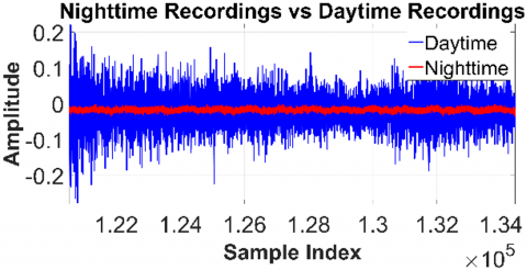
The experiments were performed in a residential room with dimensions of approximately 5 m × 4 m × 2.5 m. All recordings used for analysis were carried out under real-world conditions, where the acoustic environment included everyday household noise, outdoor traffic, or continuous fan noise from a computer and a ventilator. To better characterize the influence of these interferences, two reference cases were considered: one set of recordings conducted at night under nearly silent conditions, and another set conducted under typical everyday conditions. As shown in Figure 2, the nighttime recordings are almost free of external disturbances and primarily contain the microphones’ inherent thermal/electronic noise. This reference confirmed that the microphones themselves introduce negligible noise, and highlighted that the variations observed in daytime recordings mainly originate from realistic environmental interferences. These results demonstrate that the experimental data reflect practical everyday conditions, as intended for evaluating SSL performance in real-world scenarios.
Figure 2. Comparison of recordings captured in a quiet nighttime environment and in a daytime environment
To further analyze the recording environment, noise and signal properties of the microphones, harmonic noise components, and reverberation time were evaluated. The Root Mean Square (RMS) noise levels of the microphones were approximately 0.022 V, while the RMS signal amplitudes during hand-claps ranged between 0.065–0.089 V, yielding signal-to-noise ratios (SNR) between 8.9 dB and 12 dB. The noise floor was estimated at around −33 dB, and the gain mismatch between microphones was measured as 0.56 dB, which is acceptable for source localization tasks. DC offsets were negligible (≈ −0.018 V), and clipping was minimal (≤ 5 counts), confirming reliable acquisition without significant distortion. Low-frequency interferences at 50, 100, and 150 Hz were well below the signal level (all < −60 dB), and the high-frequency noise floor above 10 kHz was measured at about −92 dB. Reverberation time (RT60), estimated via the Schroeder method with T30 analysis, yielded values of 1.288 s, 1.193 s, and 1.595 s across the three microphones, with an average of 1.36 s. These results demonstrate that the experiments were carried out in a moderately reverberant residential environment, representative of real-life acoustic conditions in which SSL systems are expected to operate.
3.2 Data preparation
In the experimental setup, acoustic signals were recorded at various source angles and distances using the NI USB-6216 data acquisition card, which was connected to MATLAB® via the Data Acquisition Toolbox. The sampling rate was set to 48 kHz. Experiments were conducted at room temperature (≈ 20℃) and atmospheric pressure, with 343 m/s assumed as the reference speed of sound in air.
Hand clap sounds were employed as acoustic stimuli in a domestic environment. Using a protractor and a tape measure, the sound source (a human subject) was positioned at multiple angles and distances relative to the origin. At each position, the subject produced a hand clap, and the resulting acoustic data were recorded for further analysis. Data were recorded for scenarios where the sound source was positioned at different angles and distance values between 0 and 360 degrees relative to the origin. As shown in Figure 1, the coordinate system was defined such that Microphone 2 pointed in the +y direction, Microphone 1 in the –x and –y directions, and Microphone 3 in the +x and –y directions. The center of the platform was aligned with the protractor’s origin, which served as the reference for all measurements.
To minimize the effect of environmental noise and irrelevant frequency components, 5th-order band-pass Butterworth filter (100–8000 Hz) was applied to the raw recordings. Low-frequency components (e.g., room hum) and high-frequency components (e.g., electronic noise) were attenuated.
Since the recordings were obtained in a home environment, potential factors such as background noise or slight inaccuracies in positioning could affect data quality. To mitigate this, ten recordings were taken for each source position, and the one with the clearest signal onset and highest signal-to-noise ratio was selected. In total, 1551 recordings were collected at various angles and distances for subsequent SSL analysis.
3.3 Proposed model
In this section, we present the proposed method for SSL. Accurate localization relies on the acoustic signals received by the microphones, and the method estimates the source position by exploiting the time delays between these signals. The following subsections provide details on the time delay estimation and the geometric analysis underlying the approach.
3.3.1 Time delay estimation
SSL commonly relies on Time Delay Estimation (TDE) due to its proven effectiveness in determining the direction of acoustic sources. When a sound is emitted, it arrives at each microphone in an array at slightly different times and with varying waveform characteristics, depending on their spatial positions. These time differences provide crucial information for estimating the source location.
In this study, time delays between microphone signals were computed using the finddelay() function in MATLAB®. This function employs a cross-correlation-based algorithm to determine the delay between two signals. Cross-correlation measures the similarity between two signals by assessing how well they match when one is shifted in time relative to the other. The algorithm computes this similarity by summing the products of the two signals at various time shifts. The cross-correlation function $R_{x y}$ for two discrete time signals x[n] and y[n] is defined by Eq. (1) as [33]:
$R_{x y}[k]=\sum_{n=-\infty}^{\infty} x[n] * y[n+k]$ (1)
where, $k$ is the lag index and the sum is taken over all time indices $n$. The $k$ value, where $R_{x y}[k]$ is the highest, gives the delay between two signals in terms of the number of samples. Time delay estimated in samples was converted into seconds using the sampling period. The conversion of the delay in samples to the delay in seconds is defined as follows with Eq. (2) as:
Delay in Seconds $=m * T_s$ (2)
where, $T_s$ denotes sampling period.
3.3.2 Geometric analysis
In this section, a novel method based on geometric analysis is proposed for two-dimensional sound source localization. The proposed method utilizes distance measurements in meters instead of time-delay estimates in seconds. The time delays calculated in seconds in the previous section were converted into distance values using the assumed speed of sound. This conversion was defined in Eq. (3) as follows
$d_{-} c=$ Delay in Seconds $* c$ (3)
where, $c$ is the speed of sound in air and $d_{-} c$ is distance in meter calculated by using $c$. These distance differences for microphone pairs are referred to as $d_{12}, d_{13}, d_{32}$ in the following sections.
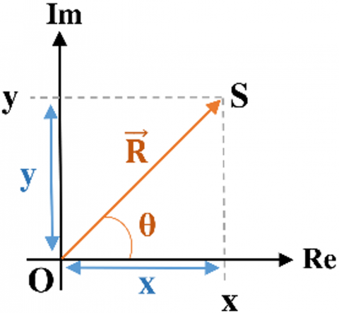
The position of any point can be defined with respect to a given reference. Based on this principle, the proposed method assumes that the location of a stationary sound source can be estimated with geometric techniques using two dimensional vectors. As illustrated in Figure 3, the position of point S relative to the origin O is represented by the position vector $\vec{R}$.
Figure 3. A position of a point
In polar form, this vector can be expressed as given by Eq. (4).
$\vec{R}=|\operatorname{os}|(\cos \theta \hat{\imath}+\sin \theta \hat{\jmath})$ (4)
where, $\hat{\imath}$ and $\hat{\jmath}$ are unit vectors. Alternatively, in Cartesian coordinates, the position vector is given by Eq. (5) as:
$\vec{R}=x \hat{\imath}+y \hat{\jmath}$ (5)
where, $x$ and $y$ are the distances. Equivalently, the position can be represented in the complex plane as given by Eq. (6).
$R=x+i y$ (6)
where, $i$ denotes the unit imaginary number.
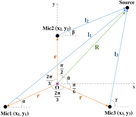
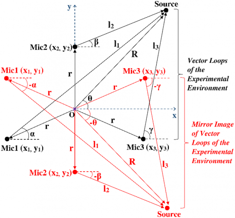
The proposed method models the position vectors of the sound source as forming closed-loop polynomials, analogous to loop closure equations. This formulation enables a novel geometric framework for SSL. As illustrated in Figure 4, the static vectors representing the position of the sound source form vector loops, and the equations that describe the closure of these loops are referred to as loop closure equations. The proposed method for SSL was performed by setting up equations similar to loop closure equations.
Figure 4. Vector loops of the experimental environment
In Figure 4, the point marked with the purple x represents the origin. Microphone1, Microphone2, Microphone3 and Sound Source was denoted as Mic1, Mic2, Mic3, Source respectively. The microphones positions were given in $\left(x_m, y_n\right)$ coordinates, and their distances from the origin are equal, shown as $r$. The distances from the origin and microphones to the sound source were represented as $R$, $l_1$, $l_2$ and $l_3$. The angles of the distances from the origin and microphones to the source with respect to the horizontal is defined as θ, α, β, γ, respectively. These angle values were measured counterclockwise to be positive.
The coordinate system was defined with the x- and y-axes shown in Figure 1, with point O was selected as the origin. The vector from point O to Mic1 was denoted as $\overrightarrow{O M \iota c 1}$ and similarly, the other vectors were defined in the same manner. According to these assumptions, the vector loops were specified as given by Eqs. (7)-(9) as:
$\overrightarrow{ { OMıc1 }}+\overrightarrow{ { Mvc1Source }}=\overrightarrow{ { OSource }}$ (7)
$\overrightarrow{ { OMıc2 }}+\overrightarrow{{ Mıc2Source }}=\overrightarrow{ { OSource }}$ (8)
$\overrightarrow{ { OMıc3 }}+\overrightarrow{ { Mvc3Source }}=\overrightarrow{ { OSource }}$ (9)
Using the parameters illustrated in Figure 4 and applying Euler’s formula, these vector loops were expressed in parametric form as presented in Eqs. (10)-(12).
$r e^{i\left(\frac{7 \pi}{6}\right)}+l_1 e^{i \alpha}=R e^{i \theta}$ (10)
$r e^{i\left(\frac{\pi}{2}\right)}+l_2 e^{i \beta}=R e^{i \theta}$ (11)
$r e^{i\left(\frac{11 \pi}{6}\right)}+l_3 e^{i \gamma}=R e^{i \theta}$ (12)
where, $r$ is the length of the microphone arms, $l_i$ is defined as the distance of the sound source to the $i^{t h}$ microphone and $R$ is the distance of sound source to the origin point.
To extend this framework, a virtual mirror was assumed along the x-axis. As shown in Figure 5, the black vectors represent the real vector loops from Figure 4, whereas the red vectors illustrate their mirrored counterparts. Each real vector loop in Figure 4 has a corresponding mirrored loop in Figure 5, forming a symmetric representation of the system. The original vector loops and their mirror images have identical magnitudes; however, in the mirror image representation, angles with respect to the horizontal axis are measured clockwise and considered negative.
Figure 5. Mirror image of vector loops of the experimental environment
Similar to those previously derived from the real vectors, the complex conjugates of the loop closure equations given in Eqs. (10)-(12) were obtained from the mirror image and defined by Eqs. (13)-(15).
$r e^{-i\left(\frac{7 \pi}{6}\right)}+l_1 e^{-i \alpha}=R e^{-i \theta}$ (13)
$r e^{-i\left(\frac{\pi}{2}\right)}+l_2 e^{-i \beta}=R e^{-i \theta}$ (14)
$r e^{-i\left(\frac{11 \pi}{6}\right)}+l_3 e^{-i \gamma}=R e^{-i \theta}$ (15)
By analytically solving the loop closure equations and their conjugates, the distance $R$ from the origin to the source was expressed in terms of different microphone parameters, as shown in Eqs. (16)-(18).
$R=\sqrt{r^2+2 r l_1 \cos \left(\frac{7 \pi}{6}-\alpha\right)+l_1^2}$ (16)
$R=\sqrt{r^2+2 r l_2 \sin (\beta)+l_2^2}$ (17)
$R=\sqrt{r^2+2 r l_3 \cos \left(\frac{11 \pi}{6}-\gamma\right)+l_3^2}$ (18)
In addition to the loop closure equations, the Cosine Theorem was applied in Figure 4 and according to the Cosine Theorem, the distances $l_1$, $l_2$, $l_3$ and $R$ were obtained. The inter microphone distance differences were then written in terms of $l_1$, $l_2$, $l_3$ as in Eqs. (19)-(21).
$d_{12}=l_1-l_2$ (19)
$d_{13}=l_3-l_1$ (20)
$d_{32}=l_3-l_2$ (21)
The distances $l_1$, $l_2$, $l_3$ were also calculated with Euclidean distance, as given in Eqs. (22)-(24), where the sound source position is determined as $(R * \cos (\theta), R * \sin (\theta))$.
$l_1=\sqrt{\left(R \cos (\theta)-x_1\right)^2+\left(R \sin (\theta)-y_1\right)^2}$ (22)
$l_2=\sqrt{\left(R \cos (\theta)-x_2\right)^2+\left(R \sin (\theta)-y_2\right)^2}$ (23)
$l_3=\sqrt{\left(R \cos (\theta)-x_3\right)^2+\left(R \sin (\theta)-y_3\right)^2}$ (24)
where, $R$ is the distance from the origin to the source, $\theta$ is the positive angle between $R$ and the horizontal axis and $x_i$, $y_i$ are the cartesian coordinates of the $i^{\text {th }}$ microphone.
The time delays were also expressed in terms of the newly calculated $l_1$, $l_2$, $l_3$ values as shown in Eqs (25)-(27).
$\begin{gathered}d_{12}=\sqrt{\left(R \cos (\theta)-x_1\right)^2+\left(R \sin (\theta)-y_1\right)^2}-\sqrt{\left(R \cos (\theta)-x_2\right)^2+\left(R \sin (\theta)-y_2\right)^2}\end{gathered}$ (25)
$\begin{gathered}d_{13}=\sqrt{\left(R \cos (\theta)-x_3\right)^2+\left(R \sin (\theta)-y_3\right)^2}-\sqrt{\left(R \cos (\theta)-x_1\right)^2+\left(R \sin (\theta)-y_1\right)^2}\end{gathered}$ (26)
$\begin{gathered}d_{32}=\sqrt{\left(R \cos (\theta)-x_3\right)^2+\left(R \sin (\theta)-y_3\right)^2}-\sqrt{\left(R \cos (\theta)-x_2\right)^2+\left(R \sin (\theta)-y_2\right)^2}\end{gathered}$ (27)
To solve these nonlinear equations, the fsolve() function in MATLAB® was employed. The solution process was performed in multiple stages: subsets of the equations were first solved to obtain preliminary estimates, which were subsequently refined by solving the complete system.
The Levenberg–Marquardt algorithm was selected as the numerical solver within fsolve(). This hybrid optimization technique combines the advantages of gradient descent and Gauss–Newton methods, enabling stable convergence when far from the initial estimate and faster convergence near the solution. The algorithm’s damping parameter ensures robustness by dynamically adjusting the step size. In this study, the maximum number of iterations was limited to 1000, and both function and step tolerances were set to 10-12. With these settings, the nonlinear systems were solved successfully, yielding the source position estimates.
To validate the proposed method, an ANN was trained using the same dataset, providing a comparative benchmark against the analytical results.
3.4 Artificial Neural Network (ANN) model
In this section, ANN model used for performance comparison was explained. In this study, a feedforward artificial neural network architecture was employed to estimate the direction and distance of a sound source based on time delay measurements between microphones. The dataset comprised a total of 1551 recordings. These samples were grouped in sets of three, from which one instance was randomly selected as the test data, while the remaining two were used for training. This sampling strategy resulted in 1034 training samples and 517 test samples. The ANN was trained exclusively using the training dataset, and its performance was evaluated on the separate test dataset to ensure unbiased assessment. In the neural network model developed for this study, the inputs consist of the true time delays between microphone pairs, expressed in meters, and the Cartesian coordinates of the microphones. As outputs, the network was trained to estimate the radial distance from the origin to the sound source and the positive horizontal angle relative to the x-axis. Based on these predicted values, the two-dimensional Cartesian coordinates (x,y) of the sound source were subsequently computed.
The implemented ANN featured a feedforward structure with three hidden layers. These hidden layers comprised 18, 27, and 10 neurons respectively. The activation functions selected for the hidden layers were the logarithmic sigmoid function for the first layer, the radial basis function for the second layer, and the linear function for the third layer. Several alternative architectures and hyperparameter settings were explored during preliminary tests, and the selected network (with three hidden layers of 18, 27, and 10 neurons) consistently yielded the best performance among the tested options. However, given the virtually infinite range of possible configurations, it cannot be claimed with certainty that this architecture represents the global optimum. Rather, it reflects the most effective structure identified within the practical constraints of this study.
The Levenberg–Marquardt backpropagation algorithm was utilized as the training algorithm due to its proven efficiency in nonlinear regression problems. Prior to training, all input and output features were normalized to enhance training convergence and ensure consistent network behavior. The normalization process was applied uniformly across both training and testing datasets. The ANN was then trained and evaluated exclusively using these normalized data values to ensure compatibility and generalization.
The obtained results using proposed method and ANN are given in the next section.
In this study, the performance of the developed model in predicting angle, distance, and position was evaluated using multiple error metrics. A total of 1551 data samples were utilized, with 1034 allocated for training and 517 reserved for testing. The obtained results compare the prediction performance of the proposed method with an ANN-based model on the test dataset, as presented in the following subsections. To assess the methods' performance, the following metrics were employed: Euclidean Distance Error, Root Mean Square Error (RMSE), Mean Percentage Error (MPE), Mean Absolute Percentage Error (MAPE), Mean Absolute Error (MAE), and Variance Accounted For (VAF). Among the evaluation metrics used in this study, only the formulation of VAF is presented below, as the others are widely used and well known in the literature. VAF is used to evaluate the proportion of variance in the actual data explained by the predicted data. When the predicted and actual values are identical, the VAF yields 100%; as the differences between them increase, the VAF value decreases. It is computed as follows [34] with Eq. (28).
$V A F_i=\left(1-\frac{\operatorname{var}\left(y_i-\hat{y}_i\right)}{\operatorname{var}\left(y_i\right)}\right) * 100$ (28)
where, $y_i$ and $\hat{y}_i$ are actual and predicted values for the $i^{\text {th }}$ component.
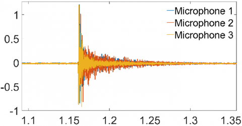
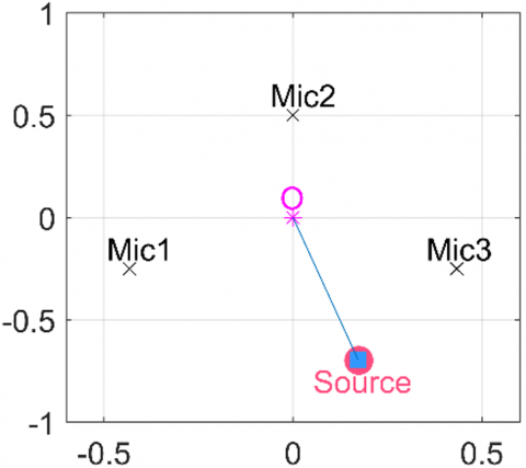
Figure 6 demonstrates the SSL capability of the proposed method. Figure 6(a) displays the signals received by the microphones when the sound source is positioned at 284° and 0.72 meters from the origin. The corresponding localization result, presented in Figure 6(b), shows the estimated position at -76.0771° (equivalent to 283.9229° when converted to a 0-360° scale) and 0.7187 meters, with a Euclidean positioning error of merely 0.0016 meters.
(a) Signals reaching the microphones
(b) Result obtained using these signals
Figure 6. Microphone signals and result
In Figure 6(b), the truth and estimated positions are marked by a red circle and blue square, respectively, visually confirming the method's precision.
For a systematic performance comparison, both the proposed method and ANNs were employed to estimate the following parameters of the sound source relative to the microphone array origin:
• Angular position (θ): The angle between the sound source and the reference axis (i.e., the positive x-axis) of the microphone array, measured in the horizontal plane.
• Radial distance (R): The Euclidean distance between the sound source and the origin of the microphone array.
• Cartesian coordinates (x, y): The 2D position of the sound source, calculated from the estimated angular position and radial distance.
While performance metrics (Euclidean Distance Error, RMSE, MAE, MPE, MAPE, and VAF) were computed for both training and test datasets, only the test results are presented here to ensure unbiased evaluation. The comparative analysis of these metrics, detailed in Tables 1-5, reveals critical insights into each method's localization accuracy and robustness.
4.1 Angular estimation performance
Table 1 summarizes the angular estimation errors, in degrees, based on the test dataset. The proposed method achieved RMSE of 1.0365°, which is considerably lower than the RMSE of 4.5898° obtained by the ANN model. This remarkable difference indicates the high accuracy of the proposed method in estimating angular direction. Furthermore, the proposed method achieved a lower MAE of 0.6004° which indicates that its predictions are significantly more stable and closer to the actual values.
In terms of relative error metrics, the proposed method once again outperformed the ANN model. The MAPE was limited to 0.7659%, which was significantly lower than the 6.6176% observed in the ANN model. Similarly, the MPE was found to be 0.0914%, indicating that systematic bias in the predictions of the proposed method is nearly negligible.
Lastly, the VAF value reached 99.99%, demonstrating that the model has strong alignment with the ground truth in angle estimation tasks.
Table 1. Angular estimation error metrics on test data
|
Models |
RMSE |
MPE |
MAPE |
MAE |
VAF |
|
Proposed Method |
1.0365 |
0.0914 |
0.7659 |
0.6004 |
99.9927 |
|
ANN |
4.5898 |
5.6705 |
6.6176 |
0.7935 |
99.8553 |
4.2 Distance estimation performance
Table 2 presents the error metrics related to the predicted distance values on the test dataset. The proposed method yielded a RMSE of 0.0080 meters, indicating a lower level of error compared to the ANN model, which reported 0.0122 meters. Although the ANN slightly outperforms the proposed method in terms of MAE in angle estimation (0.0058° vs. 0.0063°), this difference is minimal. Regarding percentage-based error metrics, the ANN achieves a lower MAPE (1.2099%) than the proposed method (1.4971%), but exhibits a higher MPE (0.2287%) compared to the proposed method’s more balanced and nearly unbiased result (-0.3064%). This suggests that, on average, the ANN tends to slightly overestimate, whereas the proposed method provides a more centered estimation around the ground truth.
VAF reached 99.9586%, demonstrating a high level of consistency and reliability in the model’s distance prediction capability.
In summary, while the ANN provides marginal improvements in average angular and percentage-based errors, the proposed method offers more robust and reliable performance in terms of absolute spatial accuracy and model generalization.
Table 2. Distance estimation error metrics on test data
|
Models |
RMSE |
MPE |
MAPE |
MAE |
VAF |
|
Proposed Method |
0.0080 |
-0.3064 |
1.4971 |
0.0063 |
99.9586 |
|
ANN |
0.0122 |
0.2287 |
1.2099 |
0.0058 |
99.9019 |
4.3 Estimation performance of the x coordinate
Table 3 presents the error metrics related to the estimation of the x coordinate of the source position. The proposed method achieves the lowest RMSE of 0.0073 meters and the highest VAF value of 99.9821%, indicating superior overall accuracy and model fit. Although the ANN demonstrates a slightly better MAE of 0.0051 degrees compared to 0.0056 degrees for the proposed method, this marginal difference in MAE is outweighed by the proposed method’s significantly lower RMSE and higher VAF.
These results suggest that the proposed method provides more reliable and consistent predictions, particularly in capturing the overall distribution and minimizing larger errors, whereas the ANN may offer slightly better average-case performance. Therefore, in terms of robust and precise estimation of the x-coordinate, the proposed approach demonstrates a clear advantage over the ANN model.
Table 3. Estimation performance of x coordinate on test data
|
Models |
RMSE |
MAE |
VAF |
|
Proposed Method |
0.0073 |
0.0056 |
99.9821 |
|
ANN |
0.0112 |
0.0051 |
99.9573 |
4.4 Estimation performance of the y coordinate
Table 4 summarizes the estimation errors for the y-axis coordinate of the source location. The proposed method consistently outperformed the ANN model in all evaluation metrics. Notably, the RMSE was measured as 0.0070 meters, which is nearly half the corresponding error observed in the ANN model. This result highlights the superior reliability of the proposed method in two-dimensional position estimation tasks.
Table 4. Estimation performance of y coordinate on test data
|
Models |
RMSE |
MAE |
VAF |
|
Proposed Method |
0.0070 |
0.0052 |
99.9678 |
|
ANN |
0.0139 |
0.0070 |
99.8742 |
4.5 Euclidean distance error
Finally, the overall positional accuracy of both models was evaluated using the Euclidean Distance Error. As presented in Table 5, the proposed method produced lower average errors for both the training and test datasets compared to the ANN model. These results indicate that the proposed method has a strong generalization ability and maintains consistent performance across different data subsets.
All these findings, when evaluated together, demonstrate that the proposed method achieves lower error rates and higher data compatibility compared to the ANN model in both angle and location estimations. Among the evaluated error metrics, the Euclidean distance error stands out as the most critical indicator to evaluate the overall localization performance. Unlike component based metrics such as angular or percentage errors, the Euclidean distance directly quantifies the spatial deviation between the estimated and true positions. Therefore, it provides a comprehensive measure of localization accuracy. In this context, the proposed method outperforms the ANN, producing significantly lower Euclidean error, which highlights its superior ability in precise position estimation. This result is particularly important for real-world applications where minimizing absolute spatial error is essential.
Table 5. Euclidean distance errors for training and test datasets
|
Models |
Euclidean Distance Error (m) Train Data |
Euclidean Distance Error (m) Test Data |
|
Proposed Method |
0.0088 |
0.0085 |
|
ANN |
0.0093 |
0.0096 |
The present study has several limitations that should be acknowledged. First, the experimental data were collected exclusively in domestic indoor environment with naturally occurring noise and reverberation. While these conditions provide a realistic representation of everyday scenarios, the dataset does not include outdoor environments, industrial spaces, or other complex acoustic contexts. As a result, the generalizability of the findings to broader conditions cannot be fully ensured.
Second, the proposed geometric analysis method has certain constraints. It relies on three microphones arranged in a triangular configuration, which provides the minimum spatial diversity necessary for unique 2D localization. Moreover, in environments with strong reverberation, overlapping sound sources, or rapidly changing acoustic conditions, the robustness of the proposed method may degrade compared to controlled scenarios.
Furthermore, although the proposed method demonstrated real-time feasibility in MATLAB®, with an average processing time of approximately 98 ms for a 3-second input signal (3.3% of the recording duration) on an Intel i7-6700HQ CPU with 16 GB RAM, several practical limitations should be acknowledged. First, the current implementation was tested only on a general-purpose laptop processor, and performance may vary when deployed on resource-constrained embedded platforms such as ARM processors or FPGAs. Second, hardware compatibility and optimization for low-power devices were not investigated in this study. Third, the proposed geometric method was specifically designed for a triangular configuration of three microphones, which ensures the minimum spatial diversity for 2D localization. Extending the method to larger or irregular microphone arrays would require additional adaptations in the algorithm and may increase computational complexity. These considerations highlight the need for further validation and optimization to ensure robust applicability in real-world embedded systems.
Third, the ANN baseline used for comparison also has limitations that influenced its performance. The underperformance of the ANN model in this specific study can be primarily attributed to two factors. First, the scale of the dataset: while the available 1,034 training and 517 test samples were sufficient to validate the proposed geometric method, they are relatively limited for data-driven models like ANNs, which typically require much larger and more diverse datasets to achieve robust generalization. This likely contributed to overfitting on the training set and reduced accuracy on unseen data. Second, although several ANN architectures were explored and the best-performing configuration was selected, the nearly infinite hyperparameter search space (e.g., neuron counts, activation functions, learning rates) makes it infeasible to guarantee a globally optimal solution within the scope of this study. Consequently, the observed performance gap does not necessarily indicate a fundamental weakness of neural networks for SSL, but rather reflects the practical challenges of applying them effectively with limited data and computational resources. Future work will therefore focus on expanding the dataset and conducting a more comprehensive architecture and hyperparameter search to enable a fairer and more definitive comparison.
Future work will focus on addressing these limitations, including optimizing the algorithm for embedded real-time platforms and ensuring scalability for larger microphone arrays. Expanding the dataset to include outdoor and industrial scenarios, as well as more complex noise conditions, will provide further insights into the method’s generalizability. Additionally, extending the evaluation to alternative microphone configurations, including irregular or larger arrays, will help to better assess scalability. Finally, combining the proposed geometric approach with machine learning or adaptive signal processing techniques may improve robustness and accuracy in challenging acoustic environments.
In this study, a new geometric method was proposed to estimate the angular direction, radial distance, and two-dimensional position of an acoustic source using a limited number of input features. The performance of the proposed method was thoroughly evaluated and compared against a traditional ANN model using a dataset of 1551 samples.
The experimental results consistently demonstrated the superior performance of the proposed method over the ANN baseline. Specifically, our approach achieved a significantly lower angular RMSE of 1.0365° compared to the ANN's 4.5898°, while also proving more accurate in distance estimation and coordinate prediction. The observed performance gap can be primarily attributed to the ANN's reliance on large datasets and its sensitivity to hyperparameter tuning, which hinder its generalization capabilities under the limited-data conditions of this study. In contrast, our proposed geometric method showed greater robustness and interpretability, achieving consistent and accurate results with a small dataset and an affordable hardware setup. The successful implementation of the entire system using consumer-grade hardware in a domestic setting further highlights the practicality and feasibility of our approach for real-world sound localization applications without the need for expensive equipment or controlled laboratory conditions. Overall, the findings suggest that the proposed method provides a reliable and practical solution for SSL.
Future studies will aim to extend the approach to three-dimensional localization and real-time operation. To achieve 3D localization, additional recordings that cover different elevation angles will be collected. For real-time use, the algorithm will need to be optimized and tested on embedded platforms such as ARM-based processors or FPGAs, with particular attention to computational efficiency. Moreover, the robustness of the method will be examined in more complex acoustic environments, including reverberant rooms and scenarios with multiple sources, through the use of larger and more diverse datasets. These efforts are expected to support the broader applicability and scalability of the method in real-world conditions.
|
c |
speed of sound |
|
dab |
distance difference between Microphone a and Microphone b |
|
la |
distance from the Microphone a to the sound source |
|
r |
distance from the origin to the microphones |
|
R |
distances from the origin to the sound source |
|
Ts |
sampling period |
|
Greek symbols |
|
|
$\alpha$ |
angle between the distance from Microphone 1 to the source and the horizontal axis |
|
$\beta$ |
angle between the distance from Microphone 2 to the source and the horizontal axis |
|
$\gamma$ |
angle between the distance from Microphone 3 to the source and the horizontal axis |
|
θ |
angle between the distance from the origin to the source and the horizontal axis |
|
Subscripts |
|
|
a, b |
indices representing microphone numbers (1, 2 or 3) |
|
s |
second (time unit) |
[1] Poschadel, N., Preihs, S., Peissig, J. (2025). Investigations on higher-order spherical harmonic input features for deep learning-based multiple speaker detection and localization. EURASIP Journal on Audio, Speech, and Music Processing, 2025(1): 7. https://doi.org/10.1186/s13636-025-00393-7
[2] Jung, I.J., Ih, J.G. (2021). Combined microphone array for precise localization of sound source using the acoustic intensimetry. Mechanical Systems and Signal Processing, 160: 107820. https://doi.org/10.1016/j.ymssp.2021.107820
[3] Padois, T., Doutres, O., Sgard, F., Berry, A. (2019). Optimization of a spherical microphone array geometry for localizing acoustic sources using the generalized cross-correlation technique. Mechanical Systems and Signal Processing, 132: 546-559. https://doi.org/10.1016/j.ymssp.2019.07.010
[4] Ma, H., Shang, T., Li, G., Li, Z. (2022). Low-frequency sound source localization in enclosed space based on time reversal method. Measurement, 204: 112096. https://doi.org/10.1016/j.measurement.2022.112096
[5] Chen, L., Chen, G.T., Huang, L., Choy, Y.S., Sun, W.Z. (2022). Multiple sound source localization, separation, and reconstruction by microphone array: A DNN-based approach. Applied Sciences, 12(7): 3428. https://doi.org/10.3390/app12073428
[6] Khan, A., Waqar, A., Kim, B., Park, D. (2025). A review on recent advances in sound source localization techniques, challenges, and applications. Sensors and Actuators Reports, 9: 100313. https://doi.org/10.1016/j.snr.2025.100313
[7] Xu, K., Zong, Z., Liu, D., Wang, R., Yu, L. (2025). Deep learning-based sound source localization: A review. Applied Sciences, 15(13): 7419. https://doi.org/10.3390/app15137419
[8] Zhao, X., Liu, B., Shi, H. (2021). Sound source localization method by using a single moving microphone and inner product calculation. Applied Acoustics, 177: 107919. http://doi.org/10.1016/j.apacoust.2021.107919
[9] Zhang, Y., Wang, Z., Wang, W., Guo, Z., Wang, J. (2017). SOLO: 2D localization with single sound source and single microphone. In 2017 IEEE 23rd International Conference on Parallel and Distributed Systems (ICPADS), Shenzhen, China, pp. 787-790. http://doi.org/10.1109/ICPADS.2017.00108
[10] Saxena, A, Ng, Y.A. (2009). Learning sound location from a single microphone. In 2009 IEEE International Conference on Robotics and Automation, Kobe, Japan, pp. 1737-1742. http://doi.org/10.1109/ROBOT.2009.5152861
[11] Flood, G., Elvander, F. (2024). Multi-source localization and data association for time-difference of arrival measurements. In 2024 32nd European Signal Processing Conference (EUSIPCO), Lyon, France, pp. 111-115. http://doi.org/10.23919/EUSIPCO63174.2024.10715317
[12] Xiong, W., Schindelhauer, C., So, H.C., Bordoy, J., Gabbrielli, A., Liang, J. (2021). TDOA-based localization with NLOS mitigation via robust model transformation and neurodynamic optimization. Signal Processing, 178: 107774. http://doi.org/10.1016/j.sigpro.2020.107774
[13] Zhang, B., Hu, Y., Wang, H., Zhuang, Z. (2018). Underwater source localization using TDOA and FDOA measurements with unknown propagation speed and sensor parameter errors. IEEE Access, 6: 36645-36661. http://doi.org/10.1109/ACCESS.2018.2852636
[14] Padois, T., Sgard, F., Doutres, O., Berry, A. (2017). Acoustic source localization using a polyhedral microphone array and an improved generalized cross-correlation technique. Journal of Sound and Vibration, 386: 82-99. http://doi.org/10.1016/j.jsv.2016.09.006
[15] Lee, R., Kang, M.S., Kim, B.H., Park, K.H., Lee, S.Q., Park, H.M. (2020). Sound source localization based on GCC-PHAT with diffuseness mask in noisy and reverberant environments. IEEE Access, 8: 7373-7382. http://doi.org/10.1109/ACCESS.2019.2963768
[16] Firoozabadi, D.A., Irarrazaval, P., Adasme, P., Zabala-Blanco, D., Játiva, P.P., Azurdia-Meza, C. (2022). 3D multiple sound source localization by proposed t-shaped circular distributed microphone arrays in combination with GEVD and adaptive GCC-PHAT/ML algorithms. Sensors, 22(3): 1011. http://doi.org/10.3390/s22031011
[17] Villadangos, J.M., Ureña, J., García-Domínguez, J.J., Jiménez-Martín, A., Hernández, Á., Pérez-Rubio, M.C. (2021). Dynamic adjustment of weighted GCC-PHAT for position estimation in an ultrasonic local positioning system. Sensors, 21(21): 7051. http://doi.org/10.3390/s21217051
[18] Zou, Y., Liu, H. (2020). A simple and efficient iterative method for TOA localization. In ICASSP 2020 - 2020 IEEE International Conference on Acoustics, Speech and Signal Processing (ICASSP), Barcelona, Spain, pp. 4881-4884. http://doi.org/10.1109/ICASSP40776.2020.9053746
[19] Ramezani, P., Tuğfe Demir, Ö., Björnson, E. (2025). Localization in massive MIMO networks: From far-field to near-field. In Massive MIMO for Future Wireless Communication Systems: Technology and Applications. The Institute of Electrical and Electronics Engineers, Inc., pp. 123-150. http://doi.org/10.1002/9781394228331.ch5
[20] Yang, Z., Wang, K. (2023). Nonasymptotic performance analysis of direct-augmentation and spatial-smoothing ESPRIT for localization of more sources than sensors using sparse arrays. IEEE Transactions on Aerospace and Electronic Systems, 59(6): 9379-9389. http://doi.org/10.1109/TAES.2023.3317370
[21] Kasthuri, N., Balambigai, S., Yuvashree, S. (2021). Source localization for underwater acoustics using esprit algorithm. IOP Conference Series: Materials Science and Engineering, 1055(1): 012023. http://doi.org/10.1088/1757-899X/1055/1/012023
[22] Yang, C., Sun, L.L., Guo, H., Wang, Y.S., Shao, Y. (2022). A fast 3D-MUSIC method for near-field sound source localization based on the bat algorithm. International Journal of Aeroacoustics, 21(3-4): 98-114. http://doi.org/10.1177/1475472X221093711
[23] Lai, W.T., Birnie, L., Chen, X., Bastine, A., Abhayapala, T.D., Samarasinghe, P.N. (2024). Source localization by multidimensional steered response power mapping with sparse Bayesian learning. In 2024 18th International Workshop on Acoustic Signal Enhancement (IWAENC), Aalborg, Denmark, pp. 31-35. http://doi.org/10.1109/IWAENC61483.2024.10694007
[24] Feng, L., Zhang, X.L., Li, X. (2025). Eliminating quantization errors in classification-based sound source localization. Neural Networks, 181: 106679. http://doi.org/10.1016/j.neunet.2024.106679
[25] Fischer, G.K., Thiedecke, N., Schaechtle, T., Gabbrielli, A., Höflinger, F., Stolz, A., Rupitsch, S.J. (2024). Evaluation of sparse acoustic array geometries for the application in indoor localization. IEEE Journal of Indoor and Seamless Positioning and Navigation, 2: 263-274. http://doi.org/10.1109/JISPIN.2024.3476011
[26] Heydari, Z., Mahabadi, A. (2023). Real-time TDOA-based stationary sound source direction finding. Multimedia Tools and Applications, 82(26): 39929-39960. http://doi.org/10.1007/s11042-023-14741-2
[27] Toma, A., Salvati, D., Drioli, C., Foresti, G.L. (2021). CNN-based processing of acoustic and radio frequency signals for speaker localization from MAVs. In Interspeech, pp. 2147-2151. http://doi.org/10.21437/Interspeech.2021-886
[28] Zhu, H., Wan, H. (2020). Single sound source localization using convolutional neural networks trained with spiral source. In 2020 5th International Conference on Automation, Control and Robotics Engineering (CACRE), Dalian, China, pp. 720-724. http://doi.org/10.1109/CACRE50138.2020.9230056
[29] Tan, T.H., Lin, Y.T., Chang, Y.L., Alkhaleefah, M. (2021). Sound source localization using a convolutional neural network and regression model. Sensors, 21(23): 8031. http://doi.org/10.3390/s21238031
[30] Hu, F., Song, X., He, R., Yu, Y. (2023). Sound source localization based on residual network and channel attention module. Scientific Reports, 13(1): 5443. http://doi.org/10.1038/s41598-023-32657-7
[31] Correia, S.D., Tomic, S., Beko, M. (2021). A feed-forward neural network approach for energy-based acoustic source localization. Journal of Sensor and Actuator Networks, 10(2): 29. http://doi.org/10.3390/jsan10020029
[32] Yang, Z., Zhang, X., Luo, Z., Shen, T., Cui, M., Li, X. (2025). Parallel Net: Frequency-decoupled neural network for DOA estimation in underwater acoustic detection. Journal of Marine Science and Engineering, 13(4): 724. http://doi.org/10.3390/jmse13040724
[33] Oppenheim, A.V., Schafer, R.W. (2009). Discrete-Time Signal Processing. 3rd ed. Pearson.
[34] Wang, K., Zhao, W., Wu, J., Ma, S. (2025). Intelligent testing method for multi-point vibration acquisition of pile foundation based on machine learning. Sensors, 25(9): 2893. http://doi.org/10.3390/s25092893