Rupesh Mandal![]() | Ankit Prasad
| Ankit Prasad![]() | Dilshad Anwar
| Dilshad Anwar![]() | Simran Hussain
| Simran Hussain![]() | Nupur Choudhury*
| Nupur Choudhury*![]() | Anuran Patgiri
| Anuran Patgiri![]() | Shreya Smita Bhuyan
| Shreya Smita Bhuyan![]() | Mrinmoy Mayur Choudhury
| Mrinmoy Mayur Choudhury![]() | Muktanjalee Deka
| Muktanjalee Deka![]() | Jyoti Barman
| Jyoti Barman![]() | Gitu Das
| Gitu Das![]()
© 2025 The authors. This article is published by IIETA and is licensed under the CC BY 4.0 license (http://creativecommons.org/licenses/by/4.0/).
OPEN ACCESS
Cancer is ranked as 2nd life-threatening disease-causing mortality if not diagnosed efficiently. It is quiet challenging to declare a patient cancerous or non-cancerous and this process takes time. There are lots of research conducted over past few years using various deep learning approaches in order to detect oral cancer through lesion and pathological images. Going through some of the studies we came to a fact that the detection could be better with the fusion of both images and clinical data of patients. In this study, the NDB-UFES dataset-comprising 237 samples of histopathological images along with corresponding clinical data-was employed for analysis. This study utilizes the benefit of computer aided detection (CAD) using artificial intelligence, deep learning and the combined dataset resulting in multimodal architecture. The architecture is a custom CNN based where the image feature is extracted and combined with the clinical data for the model training. After the model is trained efficiently its performance is evaluated. The experimental results obtained was ~97% in training and ~93% in testing with a CNN based architecture. The classification included three classes, OSCC, leukoplakia with dysplasia and leukoplakia without dysplasia. Through this study we could conclude that clinical and demographic data may positively influence the performance of deep learning models in classification of oral cancer.
multimodal, oral cancer, deep learning, CNN, clinical data
According to WHO cancer is the 2nd leading cause of death in the World [1]. Oral cancer is the 13th most common cancer globally. The Worldwide index of oral cavity cancer is approximately 377713 new cases and 177757 deaths in 2020. It is more common in men and older people as compared to women [2]. Oral Cancer is a disease which causes uncontrollable growth of cell occurring in various parts of mouth including lips, tongue, hard and soft palate cheeks, etc. It is more prominent across India and covers almost one fourth of global incidents which is around 77,000 new case and 52,000 deaths reported annually [3]. Major cause of oral cancer is Tobacco consumption which includes betel-quid chewing, smokeless tobacco, alcohol consumption, poor oral hygiene, etc. Since it is at its peak in India, early detection is the most effective phase which can have a survival rate of 80% but after metastasis the chance drops to 30% [4].
The NDB-UFES dataset used in this study is based on Brazilian patient data; we acknowledge a broader challenge in oral cancer research: many existing datasets, such as RMDS, are region-specific, with several originating from northeastern India. These areas often exhibit distinct risk factors which include high consumption of tobacco and betel quid, increased sun exposure, and potential genetic influences that may not be representative of other populations. North-east has the highest rate of cancer with the leading cancer of oral and stomach cancer, risk factors tobacco and household burning of firewood. Madhya Pradesh is in the 8th position in leading oral cancers with risk factors of tobacco and paan masala [5]. Due to lack of resources and technologies early detection is difficult. More often, this disease is detected after the cancer has already started to spread i.e. the early stage which has 5 to 6 years of survival rate which is approximately. 69.5%. However, in the later stage the rate drops to 31.6% [6]. The occurrence of oral cancer rate in United States of America is 3% whereas in India and other Asian countries it is 30%, resulting in 48,000 Americans to get affected by oral cancer every year and 8500 people die annually due to this disease [7]. Out of all the countries that has got affected by oral cancer across Asia, North America, South America and Europe, the 10 most popular countries are China, India, the United States, Indonesia, Brazil, Pakistan, Bangladesh, Russia, Japan and Mexico [8]. The main cause of having a high death rate in oral cancer is not because it’s difficult to detect and diagnose it but because it’s usually found too late when the disease has already advanced [9]. As a result, models trained on such localized data may not generalize well across different demographic or geographic contexts. Our contribution introduces a new perspective by incorporating data from a different region, thereby enhancing diversity. However, to build models with wider applicability and stronger performance across populations, future studies should prioritize collecting and validating data from a broader and more diverse range of sources.
Specialized doctors and instructors were appointed in order to detect the cancer and they perform several practices which include collecting demographic data about the patients which include basic information such as name, age, gender, weight, height, consumption of any kind of tobacco and alcohol, infected area, size of lesion, location of lesion and a part of infected tissue to test in lab and after completion of all tests the specialist come to a conclusion about the cancer. This manual operations take time and require specialized labors, equipment and the diagnosis may vary due to technician trainings [10].
Advancements in Artificial Intelligence (AI) has shown great promise in enhancing the detection and diagnosis of oral cancer. AI techniques, particularly deep learning algorithms, have demonstrated high accuracy in identifying cancerous lesions from histopathological images. These methods not only reduce the workload on physicians but also improve diagnostic precision by analysing large datasets and recognizing patterns that might missed by the human eye [10].
In this paper we aim to shed light in the advancement of AI and deep learning approach for medical diagnosis, doctors and specialists utilize both advanced and traditional methods for cancer detection using microscopic images. Hence, we aim to apply AI techniques specifically machine learning (ML) and deep learning (DL) for efficient generalization capability of the model to unique data. CNN-based model is categorized under finest DL method for learning process over varieties of datasets. Here we introduced a multimodal architecture with combined data i.e., both image data and clinical data for training purpose. Initially the histopathological images are passed through the input layer of our Custom-CNN layers for feature extraction, and the feature map is combined with clinical data and passed through the dense layer. Furthermore, there is a detailed explanation about our research and implementation categorized in several sections. Section 2 provides some collective studies which were carried out during past few years and how technology plays an important role in medical diagnosis. All these research works have motivated us in bringing off this project as it was interesting to know that several branches of science and technologies can be merged together to conclude with a lifesaving achievement. Next, we have section 3 providing a detailed description about the dataset used for this research, methodologies used and the multimodal architecture. Lastly, we have result and conclusion in section 4 which provides a detailed explanation about the progress, achievements, challenges faced and some limitations.
There are few public datasets available, here we will use NDB-UFES an oral cancer and leucoplakia dataset composed of histopathological images and patient data for our research and implementation. This public dataset includes patient demographic data along with lesion images [11]. Artificial Intelligence enables automated and precise cancer diagnosis by analyzing histopathological images to identify, classify, and predict tumour characteristics with high accuracy [12]. Few practices were conducted and various systems were designed using AI and technologies for classifying cancers [13]. Our research includes distinguishing the cancer at an early stage, a multimodal data fusion approach using deep neural network is used for the features extraction and generate a model which can predict the cancer at an early stage.
This section provides a collective study demonstrating how researchers had used several approaches resulting in promising diagnosis accuracy. Here we offer a rigorous investigation in order to detect, summarize and evaluate the facts regarding preventing, diagnosis and treatment of oral cancer. Several studies have been carried out in coming years which include histopathological images and patient data for early detection of OSCC using deep learning models such as Xception, InceptionV3, InceptionResnetV2, NASNetLarge and DenseNet201 [6]. Random Survival Forest, Gradient Boosting, Support Vector Machine and DeepSurv are some commonly used algorithms for the pathology of oral cancer providing efficient results [14]. The histopathological images are introduced to extract the desired features for four different models (VGG16, AlexNet, ResNet50 and Inception V3) and the features are selected for further classification as well as performance analysis [15]. Advancement in AI technologies provide impressive impact as it not only assists the workers but also enhances the diagnostic precision by working on large number of datasets. Data handling and image processing with huge amount of data is possible using AI and deep learning approach [16]. Patients who are suffering with oral cancer were identified and several datasets are available publicly out of which ORCHID (ORal Cancer Histology Image Database) is one which is generated to advance the researchers in AI based analysis of oral cancer or precancer [17].
On the other hand, CNN (Convolutional Neural Network) which is in the lime lite as it is more commonly used approach for image classification, it includes various models including ResNet, DenseNet, Inception and Xception. Apart from these models EfficientNet is a high-performance image classification model scales up from base B0 to B7 and resulting in improved image recognition accuracy [18]. The researchers had developed various models with an impressive accuracy leading to more awareness and advancement in this region of oral cancer. We have transfer learning [19], DenseNet201 [20] and many more.
Thus, our research explores the advantages of supervised machine learning approaches for the diagnosis of three types of oral cancer listed as OSCC, leukoplakia with dysplasia and leukoplakia without dysplasia. The proposed model utilizes an NDB-UFES dataset [11] which contain patients with at least one lesion of oral mucosa from which the histopathological image is collected, along with this demographic data of each patient is also collected which include diagnosis, age group, skin color, tobacco use and alcohol consumption. A CNN based architecture is used which include both images based model and demographic data-based model combined as a multi model for efficient performance. The model is merged based on the path of the images and trained using the diagnosis as target variable. An overview of the related studies supporting this approach is summarized in Table 1.
Section 3 of the paper explains the dataset used and algorithms applied to the dataset for processing such as region of interest and formulating the model for experimental results. It covers a detailed explanation about the overall architecture including the multimodal approach. Section 4 provides a detailed overview about our achievements and some limitations faces during this research.
Table 1. Related works
|
Authors |
Dataset Used |
Publicly Available |
Method Used |
Accuracy |
|
Ahmad et al. [6] |
The dataset included 5192 images, with 2494 (48%) classified as normal and 2698 (52%) as malignant OSCC cases. |
Available |
Xception, Inceptionv3, InceptionResNetV2 and NASNetLarge. |
97% |
|
Vollmer et al. [14] |
Clinical, genomic, and pathology data from 406 OSCC patients in the TCGA dataset. |
Available |
Random Survival Forest, Gradient Boosting Survival Analysis, Cox PH, Fast Survival SVM, and DeepSurv. |
|
|
Deif et al. [15] |
100x (NEOR 89 images, OSCC 439 images). 400x magnification (NEOR 201 images, OSCC 495 images). |
Available |
(VGG16, AlexNet, ResNet50, and Inception V3). |
96.30% |
|
Kavyashree et al. [16] |
Microscopic images, MRI images, X-ray images, CT scan images, PET scan images and color images captured from mobile phone. |
Licensed |
SVM, AdaBoost, MLP, Random Forest, Decision Tree, etc. |
100%, 95%, 94.1%, 90%, 99.4%, etc. |
|
Lu et al. [17] |
Radiation Oncology database, Otolaryngology Head and Neck Surgery database. |
Licensed |
Linear Discriminant Analysis, Quadratic Discriminant Analysis, SVM and random Forest. |
87.5% |
|
Oya et al. [18] |
90,059 image patches were used for training and evaluation. |
Licensed |
EfficientNet B0 to B7 |
99.65% |
|
Panigrahi et al. [19] |
The Mendeley dataset consists of 89 normal histopathological images and 439 OSCC images in 100 × magnification. |
Available |
VGG16, VGG19, ResNet50, InceptionV3, and MobileNet. |
96.6% |
|
Ormeño-Arriagada et al. [20] |
1000 oral picture images were grouped into two labels-cancerous (700) and non-cancerous (300). |
Available |
DL-CNN modal using DenseNet201. |
84.70% |
|
Chaudhary et al. [21] |
ORCHID (ORal Cancer Histology Image Database). |
Licensed |
CNN models (Inception V3). |
98.54% |
|
Das et al. [22] |
Oral squamous cell carcinoma (OSCC) cells consists of oral biopsy images. |
Licensed |
CNN models (Alexnet, VGG-16, VGG-19 and Resnet-50). |
97.5% |
|
Zhou et al. [23] |
1790215 patches from 197 WSIs. |
Licensed |
SmSl. ResNet-50 and EfficientNet-B0. |
90% |
|
Wang et al. [24] |
Data were collected from clinical history, lesion photos, pathology sections and follow-up information. |
Licensed |
Autoencoder for 50 epochs and obtained feature vectors form the intermediate layers; the feature vectors were clustered using the K-means clustering methods. |
83.33% |
|
Sukegawa et al. [25] |
OSCC samples were prepared from the biopsy specimens. |
Licensed |
CNN |
80% |
|
Shavlokhova et al. [26] |
Ex vivo confocal images of OSCC. |
Licensed |
MobileNet |
96% |
|
Das et al. [27] |
89 normal and 439 cancerous types have been found in Category-1 total of 528 images. Category-2 includes 201 normal and 495 cancerous, total of 696. |
Licensed |
VGG16, VGG19, Alexnet, ResNet50, ResNet101, Mobile Net and Inception Net. |
97.82% |
|
Panigrahi and Swarnkar [28] |
The Mendeley dataset consists of 89 normal histopathological images and 439 OSCC images in 100× magnification. |
Available |
VGG16, VGG19, Inceptionv3, ResNet50, MobileNet. |
91.5%, 92.65%, 96.6%, 95.25%, 95.02% |
|
Gupta et al. [29] |
1323 histopathological images. |
Available |
SVM, K-nearest neighbours, Naïve bayes, Boosted trees. |
94.16%, 90.35%, 92.61%, 95.68% |
|
Mohan et al. [30] |
The dataset has 518 images of 100 × magnification and 696 images of 400 × magnification. |
Available |
VGG16, VGG19, ResNet18, Resnet50, ResNet101, DenseNet201. |
99.50% |
|
Bakare and Kumarasamy [31] |
Total 1224 histopathological images with 290 normal images and 934 oral cancer images. |
Available |
SVM, KNN |
98% and 83% |
|
Subhija and Reju [32] |
1,224 oral histopathology images, Imagenet, CIFAR or MNIST. |
Available |
VGG 16, ResNet 50, InceptionV3, Xception and DensNet112. |
90%, 97.66%, 86%, 85.5%, 89%. |
|
Albalawi et al. [33] |
1,224 images from 230 patients. |
Available |
EfficientNetB3 architecture. |
99.13% |
|
Ding et al. [34] |
16,200 Raman spectral data. |
Licensed |
DMFF-ResNet is used. |
93.28 % |
|
Martino et al. [35] |
Haematoxylin and Eosin (H&E) stained images. |
Licensed |
Deep learning model. |
76.67% |
3.1 Dataset description
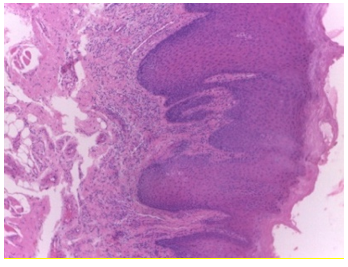
The efficiency of our research also depends on the dataset selected for implementation. The NDB-UFES dataset composed of histopathological images and patient data. The images are of different sizes with approximately 2048 × 1536 pixels. All total of 237 images in PNG format out of which 89 are leukoplakia with dysplasia, 57 are leukoplakia without dysplasia and 91 are OSCC images captured with an optical light microscope using 10x and 40x objective attached with a microscope camera. A hematoxylin-eosin stain is used in the histopathological slides from the biopsy of patients performed between 2010 and 2021 managed by Oral Diagnosis project of Federal University of Espírito Santo (NDB-UFES) [11]. The dataset contains sociodemographic data including age, gender and skin color as well as clinical data including alcohol consumption, sun exposure, tobacco use, lesion, type of biopsy, lesion surface and lesion color were also collected. The dataset has a separate patches folder consisting of 3736 patches of cancerous images as well.
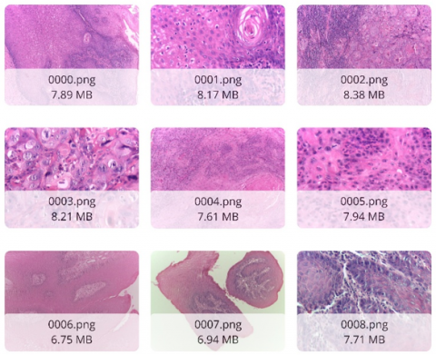
This dataset also consists of patients’ clinical and demographic information in a CSV as well as XLS format. Representative sample images are shown in Figure 1, and a snapshot of the dataset obtained from Kaggle [36] is provided in Figure 2. Table 2 below provides the data dictionary of clinical data. The CSV file consists of a total of 237 records with 17 columns.
Figure 1. Sample images
Figure 2. Snapshot of dataset from Kaggle [36]
Table 2. Data dictionary
|
Name |
Column Name |
Description |
|
ID |
public_id |
A unique ID for each sample. |
|
Filename |
path |
Histopathologic image filename. |
|
Lesion localization |
localization |
Lesion’s localization in body. (Tongue, Gingiva, Buccal mucosa, Floor of mouth, Lip, Palate). |
|
Lesion larger size |
larger_size |
Larger size of the lesion in centimeters. |
|
Diagnosis |
diagnosis |
Lesion diagnosis. (OSCC, Leukoplakia with dysplasia, Leukoplakia without dysplasia). |
|
Dysplasia severity |
dysplasia_severity |
Severity of the dysplasia in the lesion. (Mild, Severe, Moderate). |
|
Gender |
gender |
Patient’s gender. Male or Female (M, F). |
|
Age group |
Age_group |
Patient’s age group. Group 0 for ages lesser than 40 years. Group 1 for ages between 41 and 60 years, included. Group 2 for ages greater than 60 years. |
|
Skin color |
Skin_color |
Patient’s skin color. (Black, Brown, White and Others). |
|
Tobacco use |
tobacco_use |
Patient’s tobacco use. (Yes, no, Former, Not Informed). |
|
Alcohol consumption |
Alcohol_consumption |
Patient’s alcohol consumption. (Yes, no, Former, Not Informed). |
|
Sun exposure |
Sun_exposure |
Patient’s sun exposure in hours. It is -1, if not informed. |
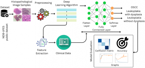
3.2 Computer aided detection
We proposed a computer-aided detection system that can assist the doctors in the interpretation of medical images. The system uses deep convolutional layers for feature extraction of lesion images and a multi model fusion methods in order to combine the image feature with clinical and demographic data of patients. As the doctors and expertise can diagnose the patient with their meta data and lesion image, we propose that this computer-aided detection system can assist them using the combination of information.
3.3 Model description
A deep learning approach CNN which contains some specific regions starting from lower layers to the higher layers to process raw pixel values of images. There are four basic layers of CNN: A convolutional layer for feature extraction and generating a feature map from the image provided as input, a max pooling layer that only targets the max features or pixel values and reduces the complexity, a flatten layer that converts the 2D or 3D matrices into 1D array and the dense layer which is the fully connected layer containing neurons inter connected with each other. The convolutional layer uses an activation function which adds non-linearity to the model, one of the activation functions used in our model was ReLU (Rectified Linear Unit). Using the combination of the above layers, a CNN model was created and it achieved better detection capability by tuning the hyperparameters. All the layers were available in the Keras library which were directly imported and used for image classification. Our work specifically considers a custom CNN model designed for specific multi model classification task. It is a traditional CNN architecture designed to address the unique requirements to integrate both image and clinical data for better results.
The convolutional layer applies a 3 × 3 filter on the input image of 224 × 224 to generate a feature map. The max pooling layer applies 2 × 2 matrix. Below are the steps that illustrate the formulation of the model:
To prepare the clinical data for training, a clear and consistent preprocessing strategy was applied. Categorical fields such as gender, tobacco use, and skin color sometimes included values like "Not Informed", instead of removing or filling these entries, they were kept and treated as valid categories to avoid losing potentially useful information. These categorical variables were then converted into numerical format using one-hot encoding, making them suitable for model input. At the same time, numerical features like lesion size and patient IDs were scaled using standard normalization so that all the values are on a similar scale. These steps were organized into a single preprocessing pipeline, which was saved for later use to ensure that the same process was carried out during testing and prediction. This helped to maintain consistency and improve the overall quality of the input data used in the multimodal model.
3.4 Model formulation
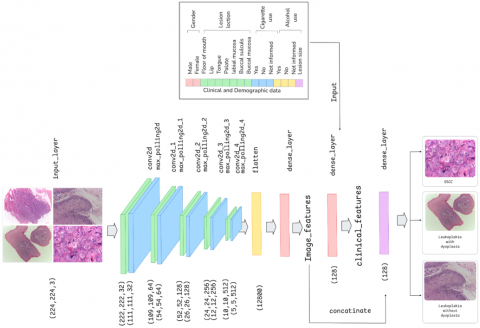
The motivation behind our research was to use a multi-model approach where histopathological images were processed by a custom CNN architecture for feature extraction, a feature map was generated at the end of the convolutional layers and was combined with clinical data. Since it’s a multimodal so the clinical data was passed at the final dense layer of the CNN architecture and combined with the feature map which was generated earlier, resulting in a merged data (i.e., both image and clinical data) for the model. Hence, the model was trained with multiple data. This approach was intended to overcome some of the challenges by being computationally effective, cost effective and providing faster training for the dataset, resulting in highly efficient diagnosis. It basically has two components. Initially the histopathological images were processed by converting the pixel values to [0,1] and were passed as input in the input layer of custom CNN layers for generation of feature map. The extracted feature map was combined with the clinical data of same patients simultaneously at the final dense layer for efficient training.
Figure 3 represents the architecture of the multimodal which was initially trained with the histopathological image dataset and the feature map was generated while passing through the custom-CNN convolutional, max pooling and flatten layers. After the feature map was successfully generated, the clinical and demographic data were introduced as input from the directory and merged with the extracted feature. The data was further trained by passing them through the dense layers for efficient result. After the model was trained efficiently an overall classification report was obtained for performance evaluation.
3.4.1 Image and clinical data fusion
The image features were combined with clinical data using a concatenate function. Below are the steps followed to concatenate both features.
Step 1: Input Data
(i) Images (224 × 224 × 3) – processed through CNN.
(ii) Clinical Data (structured/tabular format) – Processed through Dense Layer. The detailed structure of the input data used for model development is presented in Table 3.
Table 3. Input data
|
Sample |
Image (224 × 224 × 3) |
Clinical Data (Gender, Age, Smoking, etc.) |
|
1 |
000.png |
Male,40, Smoker, etc. |
|
2 |
001.png |
Female,45, Non-Smoker, etc. |
Step 2: Feature Extraction
(i) CNN extracts feature from image – Output 1D vector.
(ii) Dense Layer process clinical data – Output another 1D vector. The set of extracted features derived from the dataset is summarized in Table 4.
Table 4. Extracted features
|
Sample |
Image Features (128D) |
Clinical Data (128D) |
|
1 |
[0.5, 0.2, 0.7, ...] |
[0.1, 0.4, 0.9, ...] |
|
2 |
[0.3, 0.8, 0.6, ...] |
[0.2, 0.3, 0.5, ...] |
Step 3: Concatenation
(i) Both 128D vectors are merged into a single 256D feature vector.
(ii) Therefore, Final feature = Concatenate (image features, Clinical features). The concatenated representation of the multimodal data is provided in Table 5.
Figure 4 shows a custom convolutional neural network (CNN) architecture which is developed to extract meaningful features from histopathological images, each resized to 224 × 224 pixels with three color channels (RGB). The architecture, implemented in TensorFlow/Keras, is structured as follows:
1. Input Layer
This layer accepts raw images and resizes them to (224, 224, 3).
Table 5. Concatenated
|
Sample |
Concatenated Features (256D) |
|
1 |
[0.5, 0.2, 0.7, ..., 0.1, 0.4, 0.9, ...] |
|
2 |
[0.3, 0.8, 0.6, ..., 0.2, 0.3, 0.5, ...] |
2. Feature Extraction Blocks
The model includes three convolutional blocks, each followed by max pooling to progressively reduce spatial dimensions:
a. Block 1: 32 filters, 3 × 3 kernel, ReLU activation - MaxPooling2D (2 × 2)
b. Block 2: 64 filters, 3 × 3 kernel, ReLU activation - MaxPooling2D (2 × 2)
c. Block 3: 128 filters, 3 × 3 kernel, ReLU activation - MaxPooling2D (2 × 2)
3. Flattening Layer
The output from the final pooling layer is flattened into a 1D vector.
4. Dense Layers with Regularization
This layer captures higher-level representations and reduce overfitting, the network includes several fully connected layers with ReLU activations, dropout (0.5), and L2 regularization (λ = 0.001):
a. Dense(256) → Dropout(0.5)
b. Dense(128) → Dropout(0.5)
c. Dense(64) → Dropout(0.5)
d. Final output: Dense(128), producing a compact feature vector.
A detailed summary of the proposed model architecture is presented in Table 6.
Table 6. Model summary
|
Layer (type) |
Output Shape |
Param |
|
conv2d |
(None,64,6432) |
896 |
|
max_pooling2d |
(None, 32, 32, 32) |
0 |
|
dropout |
(None, 32, 32, 32) |
0 |
|
conv2d_1 |
(None, 32, 32, 64) |
18496 |
|
max_pooling2d_1 |
(None, 16, 16, 64) |
0 |
|
dropout_1 |
(None, 16, 16, 64) |
0 |
|
flatten |
(None, 16384) |
0 |
|
dense |
(None, 256) |
4194560 |
|
dropout_2 |
(None, 256) |
0 |
|
dense_1 |
(None, 128) |
32896 |
|
dropout_3 |
(None, 128) |
0 |
|
dense_2 |
(None, 64) |
8256 |
|
dropout_4 |
(None, 64) |
0 |
|
dense_3 |
(None, 128) |
8320 |
4.1 Classification report
Table 7 presents the performance metrics of the model obtained in our research. Since NDB-UFES dataset was used which consisted both image and clinical data, the resulted model was a multimodal. A total of 237 images were present out of which 80% were used for training the model and remaining 20% were used for testing purpose. This proposed work was implemented using Keras and TensorFlow libraries, Anaconda as the virtual environment and Python for implementation purpose. To inspect the efficacy of the proposed work, Recall, Precision, F1-score and Accuracy metric of the model were calculated.
A custom CNN model was implemented on a workstation with the following specification: Ryzen 7, 16 GB RAM and 4 GB VRAM. In order to execute, Python was used as a language. The results obtained are presented and discussed below. The prime focus of this research was to utilize the deep neural networks and obtain the features of data to design a computer aided diagnosis system.
The hyper-parameters of the model are as follows: Input size of image was 224 × 224, optimizer used was Adam, ReLu as an activation function, 200 epochs were considered with a batch size of 32 and SoftMax as a default classifier. The training accuracy obtained was ~97% and test accuracy was ~93%.
Table 7. Classification report
|
|
Precision |
Recall |
Fi-Score |
Support |
|
Leukoplakia with dysplasia |
0.89 |
0.94 |
0.92 |
18 |
|
Leukoplakia without dysplasia |
1.00 |
0.80 |
0.89 |
10 |
|
OSCC |
0.95 |
1.00 |
0.98 |
20 |
|
Accuracy |
|
|
0.94 |
48 |
|
Macro avg |
0.95 |
0.91 |
0.93 |
48 |
|
Weighted avg |
0.94 |
0.94 |
0.94 |
48 |
4.2 Plots
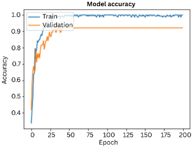
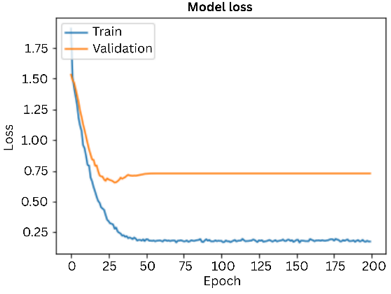
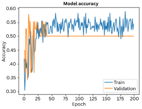
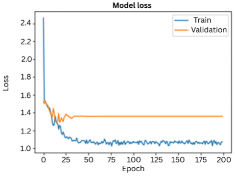
The graph given below shows the accuracy of the deep learning model of over 200 epochs for both training and validation. The graphs were plotted to evaluate how well the model learned throughout the training and testing phase. X-axis indicates the training epochs i.e., 200 and y-axis indicates accuracy of the model. Blue line represents the model’s accuracy on training data over each epoch and the orange line represents the model accuracy on the validation data over each epoch, as shown in Figure 5. Similarly, the corresponding loss curves for training and validation are presented in Figure 6.
Figure 5. Accuracy graph
Figure 6. Loss graph
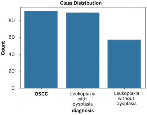
Figure 7. Class distribution
Figure 8. Confusion matrix
The figure above provides the class distribution for each type of cancer. From the graph we can imagine that out of 237 of the total number of entries, approx. 90 entities belong to OSCC, approx. 85 entities belong to leukoplakia with dysplasia and approx. 50 entities belong to leukoplakia without dysplasia, as illustrated in Figure 7.
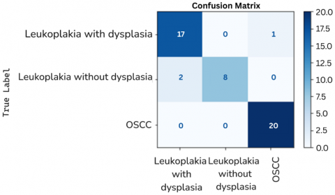
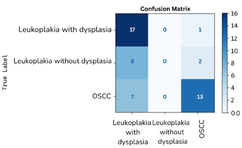
The effectiveness of this research is further confirmed using a confusion matrix as shown in Figure 8.
The x-axis i.e., the horizontal axis denotes the Predicted Labels of the model and the y-axis i.e., the vertical axis denotes the True Labels. There are total of three labels named as OSCC (Oral Squamous Cell Carcinoma), Leukoplakia with dysplasia and Leukoplakia without dysplasia. The cells in the matrix shows the number of instances that fall under a particular predicted class with the diagonal elements representing the number of correct predictions. For example, 17 instances are correctly predicted as Leukoplakia with dysplasia and only 1 instance is incorrectly predicted as OSCC i.e., the misclassifications which can be termed as off-diagonal elements. 8 instances were correctly classified as leukoplakia and 2 instances were incorrectly classified as Leukoplakia with dysplasia. Lastly 20 instances were correctly classified as OSCC and 0 instances were incorrectly classified. The above confusion matrix concludes that the model performs well in distinguishing OSCC with all the 20 instances being correctly classified but there were some misclassifications among Leukoplakia with dysplasia and Leukoplakia without dysplasia.
To evaluate the performance of the proposed model, the confusion matrix was used to compute accuracy, precision, sensitivity and specificity using the equations below. True positive (TP) and true negative (TN), false positive (FP) are the metric of confusion matrix representing correct predictions. Similarly, false positive (FP) and false negative (FN) are the metric of confusion matrix representing incorrect predictions.
Accuracy = (TP+TN)/(TP+TN+FP+FN) × 100% (1)
Precision = TP/(TP+FP) × 100% (2)
Sensitivity = TP/(TP+FN) × 100% (3)
Specificity = TN/(TN+TP) × 100% (4)
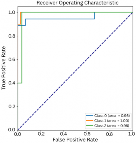
4.3 ROC curve
The graph given below shows the accuracy of the deep learning model of over 200 epochs for both training and validation, as illustrated in Figure 9. The graphs were plotted to evaluate how well the model learned throughout the training and testing phase. X-axis indicates the training epochs i.e., 200 and y-axis indicates accuracy of the model. Blue line represents the model’s accuracy on training data over each epoch and the orange line represents the model accuracy on the validation data over each epoch.
Figure 9. ROC graph
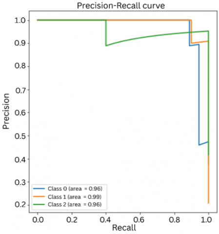
Figure 10. Precision-Recall graph
Figure 10 represents the Precision-Recall Curve i.e., the comparison of precision and recall. Class 0 is represented by blue line with an AUC value of ~96% indicating that model is effective in identifying the positive instances with high precision and recall. Class 1 is represented by orange line with an AUC value of ~99% which indicated that the model is nearly perfect. Class 2 is represented by green line with an AUC value of ~96% indicating that model performs well for the instances too.
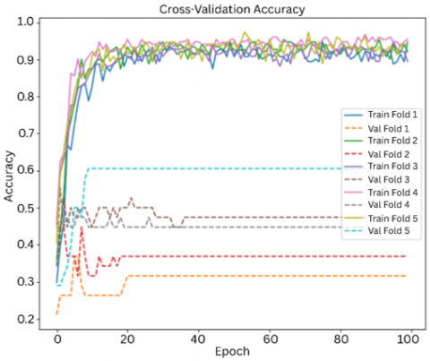
4.4 Cross validation
The model was further tested using stratified k-fold cross validation. It was necessary to address to ensure the model performs well across different subsets of data and doesn't just learn patterns from a specific split, we used 5-fold stratified cross-validation. This approach splits the dataset into five equal parts while keeping the class distribution balanced in each fold. In every round, the model was trained on four folds and tested on the remaining one. We also set aside 20% of the training data for validation during training. This allowed us to monitor performance and adjust the learning rate when needed. The process was repeated five times, and the result of each fold was averaged to get a more reliable estimate of the model’s performance and consistency.for better evaluation of the model. Each fold was evaluated with 200 epochs, batch size of 32 and with a splitting ratio of 80-20%. The average train accuracy obtained was ~85% and test accuracy was ~82%, as summarized in Table 8.
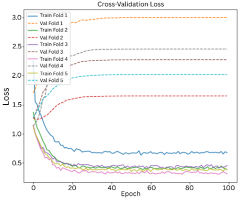
Figures 11 and 12 show the performance of multimodal in each folds.
Figure 11. Cross-validation accuracy
Figure 12. Cross-validation loss
Table 8. Result
|
Fold |
Training Accuracy |
Test Accuracy |
|
Fold 1 |
~80% |
~79% |
|
Fold 2 |
~85% |
~83% |
|
Fold 3 |
~83% |
~93% |
|
Fold 4 |
~90% |
~72% |
|
Fold 5 |
~85% |
~80% |
4.5 Single model approach
The NDB-UFES dataset consists of both images as well as patients that were used to implement a multimodal approach (Both image and demographic data trained model), but it was necessary to address how well this multimodal approach performs against a single-model approach.
The image data was further trained with the same CNN architecture so that the generalization capability of a single model can be compared with a multimodal approach. Some basic parameters used were epochs = 200, batch size = 32 and splitting ratio 80-20%.
Figure 13. Accuracy graph
The graph below shows the model performance in 100 epochs with a training accuracy of ~53% and test accuracy of ~62%. It can be seen that the model improved steadily on the training data, but validation accuracy stopped improving early. While training loss kept decreasing, validation loss stayed flat, pointing to possible overfitting. This concludes that the model learned the training data well but may not generalize as effectively to new, unseen cases, unseen cases, as shown in Figure 13 (accuracy graph) and Figure 14 (loss graph).
The confusion matrix (shown in Figure 15) on the other hand shows that the model performed well and identifies the class Leukoplakia with dysplasia, but struggles with Leukoplakia without dysplasia, often gets confused with other classes. It handles OSCC moderately well but still makes some misclassifications. This suggests that the model finds it harder to distinguish between certain lesion types, likely due to overlapping features in the data.
Figure 14. Loss graph
Figure 15. Confusion matrix
Oral Cancer is a spreading medical condition which require an early detection and treatments are crucial for better outcomes. Diagnosis supported by biopsy which involves microscopic images are quiet a common approach for confirming the presence of cancer. This proposed research aims to develop a DL based mechanism for detection and classification of three types of oral cancer i.e., OSCC, leukoplakia with dysplasia and leukoplakia without dysplasia from the histopathological images and patient’s data. The main objective was to design a computer aided diagnosis system for early prediction of cancer. To achieve this, the research employed a custom designed deep learning CNN model and this model was again customized by tuning the hyperparameters such as improving the layers, epochs, target variable, batch size, etc. This experiment aims for a multimodal approach to improve the efficacy, it was termed as multimodal as both the image data and clinical data were combined so that the model gets trained collectively. Furthermore, our proposed work explored the advantages of combining the models and provided an impressive outcome with the training accuracy of ~97% and test accuracy of ~93%. The model was successful in classifying cancer from the images, indicating the value and importance of DL approaches for oral cancer diagnosis. The proposed model provides an early detection of oral cancer resulting in early treatments. This study also aims to assist the doctors and specialists by increasing the accuracy of diagnosis, reducing workload and being cost-effective.
While the model achieved a high training accuracy of 97% and a slightly lower testing accuracy of 93%, the gap suggests a mild level of overfitting. This indicates that the model may have learned some patterns which are too specific to the training data. To help reduce this effect, techniques such as dropout layers and L2 regularization were already applied. However, further improvements could include increasing the dropout rate, pre-processing techniques, adding data augmentation, or using techniques like early stopping to prevent the model from overtraining. Our future work will try to improve the model’s generalization towards testing as it will incorporate stain normalization as pre-processing technique. Data augmentation is a bit challenging as the dataset is both image as well as clinical data and both are correlated with each other. Random augmentation may lead to shuffling of data which might affect the correlation among the data.
Some of the challenges faced during this research includes data selection as it aimed for a multimodal approach which required both image data as well as clinical data. Several datasets were selected initially for the research but they were not publicly available. Secondly there were several factors which were not aligning during the merging phase. At the end we were able to coin some of the mistakes and got our research done with impressive results.
We recognize the dataset's limited size (237 samples) and uneven class distribution where there are more OSCC cases compared to leukoplakia without dysplasia. This becomes a challenge and to reduce potential bias during training, we will be using data augmentation techniques such as image rotation, flipping, and shifting to enhance sample variety and partially address class imbalance in our future work. We did not apply traditional oversampling methods, as these can introduce noise or lead to overfitting in image-based tasks. Instead, we relied on the strength and ability of modern deep learning models to generalize well, even with limited and imbalanced datasets. In future studies, we plan to explore more targeted balancing strategies or the use of synthetic data to further improve model robustness. In context with the current research carried out, it was observed that there are very few researches conducted which utilizes the importance of clinical data with image data. With this work we will try to introduce the importance of multimodal approach over single model approach and due to which the dataset used in this research is considered as most important rather the number of entities are limited to 237 only.
After considering how our multimodal model performs in testing, there are some real-world challenges to consider. The model’s accuracy may drop if the input images are of low quality, things like poor lighting, blurriness, or different camera angles can affect results. If clinical data is missing or incomplete, it may lead to less reliable predictions since the model uses both image and patient information. Differences in how data is collected across hospitals or clinics can also impact how well the model works with new settings. To overcome these challenges, it’s very important to have consistent data collection methods, strong preprocessing strategies and fine-tune the model with local data before using it in a clinical environment.
This research can be continued in the future with new approaches including a complete comparison report on various supervised and deep learning algorithms using the same dataset and more. A collective data consisting of both images as well as clinical data can be collected and various deep learning models will be trained for a collective analysis on the performance of the models. Furthermore, we aim to continue our research utilizing the technological advancements and design a system with the most efficient deep learning models.
This research work has been supported by the Indian Council of Medical Research (ICMR) under the Project IIRP-2023-7778, in collaboration with the State Cancer Institute, Guwahati Medical College, Assam.
[1] Press Release, Press Information Bureau, India. https://pib.gov.in/PressReleasePage.aspx?PRID=2019532, accessed on Oct. 7, 2025.
[2] Oral health, World Health Organization. https://www.who.int/health-topics/oral-health, accessed on Aug. 1, 2024.
[3] Borse, V., Konwar, A.N., Buragohain, P. (2020). Oral cancer diagnosis and perspectives in India. Sensors International, 1: 100046. https://doi.org/10.1016/j.sintl.2020.100046
[4] de Lima, L.M., de Assis, M.C.F.R., Soares, J.P., Grão-Velloso, T.R., de Barros, L.A.P., Camisasca, D.R., Krohling, R.A. (2023). Importance of complementary data to histopathological image analysis of oral leukoplakia and carcinoma using deep neural networks. Intelligent Medicine, 3(4): 258-266. https://doi.org/10.1016/j.imed.2023.01.004
[5] Oral Cancer in India, National Oral Cancer Registry. https://nocr.org.in/NOCR/OralCancerinIndia, accessed on Aug. 1, 2024.
[6] Ahmad, M., Irfan, M.A., Sadique, U., Haq, I.U., Jan, A., Khattak, M.I., Ghadi, Y.Y., Aljuaid, H. (2023). Multi-method analysis of histopathological image for early diagnosis of oral squamous cell carcinoma using deep learning and hybrid techniques. Cancers, 15(21): 5247. https://doi.org/10.3390/cancers15215247
[7] Mouth and Oral Cancer Statistics, World Cancer Research Fund. https://www.wcrf.org/cancer-trends/mouth-and-oral-cancer-statistics, accessed on Oct. 7, 2025.
[8] National Center for Biotechnology Information. https://www.ncbi.nlm.nih.gov/, accessed on Oct. 7, 2025.
[9] The top 10 causes of Death. World Health Organization. https://www.who.int/news-room/fact-sheets/detail/the-top-10-causes-of-death, Accessed on Oct. 7, 2025.
[10] Ilhan, B., Lin, K., Guneri, P., Wilder-Smith, P. (2020). Improving oral cancer outcomes with imaging and artificial intelligence. Journal of Dental Research, 99(3): 241-248. https://doi.org/10.1177/0022034520902128
[11] Ribeiro-de-Assis, M.C.F., Soares, J.P., de Lima, L.M., de Barros, L.A.P., Grão-Velloso, T.R., Krohling, R.A., Camisasca, D.R. (2023). NDB-UFES: An oral cancer and leukoplakia dataset composed of histopathological images and patient data. Data in Brief, 48: 109128. https://doi.org/10.1016/j.dib.2023.109128
[12] Shao, T., Ni, P., Wang, C., Li, J., Lv, X. (2025). Prediction of pathological grade of oral squamous cell carcinoma and construction of prognostic model based on deep learning algorithm. Discover Oncology, 16(1): 976. https://doi.org/10.1007/s12672-025-02144-8
[13] Rahman, T.Y., Mahanta, L.B., Das, A.K., Sarma, J.D. (2020). Automated oral squamous cell carcinoma identification using shape, texture and color features of whole image strips. Tissue and Cell, 63: 101322. https://doi.org/10.1016/j.tice.2019.101322
[14] Vollmer, A., Hartmann, S., Vollmer, M., Shavlokhova, V., Brands, R. C., Kübler, A., Wollborn, J., Hassel, F., Couillard-Despres, S., Lang, G., Saravi, B. (2024). Multimodal artificial intelligence-based pathogenomics improves survival prediction in oral squamous cell carcinoma. Scientific Reports, 14(1): 5687. https://doi.org/10.1038/s41598-024-56172-5
[15] Deif, M.A., Attar, H., Amer, A., Elhaty, I.A., Khosravi, M.R., Solyman, A.A. (2022). Diagnosis of oral squamous cell carcinoma using deep neural networks and binary Particle Swarm optimization on histopathological images: An AIoMT approach. Computational Intelligence and Neuroscience, 2022(1): 6364102. https://doi.org/10.1155/2022/6364102
[16] Kavyashree, C., Vimala, H.S., Shreyas, J. (2024). A systematic review of artificial intelligence techniques for oral cancer detection. Healthcare Analytics, 5: 100304. https://doi.org/10.1016/j.health.2024.100304
[17] Lu, C., Lewis Jr, J.S., Dupont, W.D., Plummer Jr, W.D., Janowczyk, A., Madabhushi, A. (2017). An oral cavity squamous cell carcinoma quantitative histomorphometric-based image classifier of nuclear morphology can risk stratify patients for disease-specific survival. Modern Pathology, 30(12): 1655-1665. https://doi.org/10.1038/modpathol.2017.98
[18] Oya, K., Kokomoto, K., Nozaki, K., Toyosawa, S. (2023). Oral squamous cell carcinoma diagnosis in digitized histological images using convolutional neural network. Journal of Dental Sciences, 18(1): 322-329. https://doi.org/10.1016/j.jds.2022.08.017
[19] Panigrahi, S., Nanda, B.S., Bhuyan, R., Kumar, K., Ghosh, S., Swarnkar, T. (2023). Classifying histopathological images of oral squamous cell carcinoma using deep transfer learning. Heliyon, 9(3): e13444. https://doi.org/10.1016/j.heliyon.2023.e13444
[20] Ormeño-Arriagada, P., Navarro, E., Taramasco, C., Gatica, G., Vásconez, J.P. (2024). Deep learning techniques for oral cancer detection: Enhancing clinical diagnosis by ResNet and DenseNet performance. In International Conference on Applied Informatics, pp. 59-72. https://doi.org/10.1007/978-3-031-75144-8_5
[21] Chaudhary, N., Rai, A., Rao, A.M., Faizan, M.I., Augustine, J., Chaurasia, A., Mishra, D., Chandra, A., Chauhan, V., Kutum, R., Ahmad, T. (2023). ORCHID: A comprehensive oral cancer histology image database for histopathological analytics and diagnostics. medRxiv. https://doi.org/10.1101/2023.08.14.23294094
[22] Das, N., Hussain, E., Mahanta, L.B. (2020). Automated classification of cells into multiple classes in epithelial tissue of oral squamous cell carcinoma using transfer learning and convolutional neural network. Neural Networks, 128: 47-60. https://doi.org/10.1016/j.neunet.2020.05.003
[23] Zhou, J., Wu, H., Hong, X., Huang, Y., Jia, B., Lu, J., Cheng, B., Xu, M., Yang, M., Wu, T. (2024). A pathology-based diagnosis and prognosis intelligent system for oral squamous cell carcinoma using semi-supervised learning. Expert Systems with Applications, 254: 124242. https://doi.org/10.1016/j.eswa.2024.124242
[24] Wang, F., Song, Y.S., Xu, H., Liu, J.X., et al. (2024). Prediction of the short-term efficacy and recurrence of photodynamic therapy in the treatment of oral leukoplakia based on deep learning. Photodiagnosis and Photodynamic Therapy, 48: 104236. https://doi.org/10.1016/j.pdpdt.2024.104236
[25] Sukegawa, S., Ono, S., Tanaka, F., Inoue, Y., et al. (2023). Effectiveness of deep learning classifiers in histopathological diagnosis of oral squamous cell carcinoma by pathologists. Scientific Reports, 13(1): 11676. https://doi.org/10.1038/s41598-023-38343-y
[26] Shavlokhova, V., Sandhu, S., Flechtenmacher, C., Koveshazi, I., et al. (2021). Deep learning on oral squamous cell carcinoma ex vivo fluorescent confocal microscopy data: A feasibility study. Journal of Clinical Medicine, 10(22): 5326. https://doi.org/10.3390/jcm10225326
[27] Das, M., Dash, R., Mishra, S.K. (2023). Automatic detection of oral squamous cell carcinoma from histopathological images of oral mucosa using deep convolutional neural network. International Journal of Environmental Research and Public Health, 20(3): 2131. https://doi.org/10.3390/ijerph20032131
[28] Panigrahi, S., Swarnkar, T. (2020). Machine learning techniques used for the histopathological image analysis of oral cancer–A review. The Open Bioinformatics Journal, 13(1). https://doi.org/10.2174/1875036202013010106
[29] Gupta, R.K., Manhas, J., Kour, M. (2022). Hybrid feature extraction based ensemble classification model to diagnose oral carcinoma using histopathological images. Journal of Scientific Research, 66(3): 219-226. https://doi.org/10.37398/JSR.2022.660327
[30] Mohan, R., Rama, A., Raja, R.K., Shaik, M.R., Khan, M., Shaik, B., Rajinikanth, V. (2023). OralNet: Fused optimal deep features framework for oral squamous cell carcinoma detection. Biomolecules, 13(7): 1090. https://doi.org/10.3390/biom13071090
[31] Bakare, Y.B., Kumarasamy, M. (2021). Histopathological image analysis for oral cancer classification by support vector machine. International Journal of Advances in Signal and Image Sciences, 7(2): 1-10. https://doi.org/10.29284/ijasis.7.2.2021.1-10
[32] Subhija, E.N., Reju, V.G. (2023). An image patch selection algorithm for the detection of Oral Squamous Cell Carcinoma using textural and morphological features. Research Square. https://doi.org/10.21203/rs.3.rs-3085184/v1
[33] Albalawi, E., Thakur, A., Ramakrishna, M.T., Bhatia Khan, S., SankaraNarayanan, S., Almarri, B., Hadi, T.H. (2024). Oral squamous cell carcinoma detection using EfficientNet on histopathological images. Frontiers in Medicine, 10: 1349336. https://doi.org/10.3389/fmed.2023.1349336
[34] Ding, J.Y., Yu, M.X., Zhu, L.Q., Zhang, T., Xia, J.B., Sun, G.H. (2020). Diverse spectral band-based deep residual network for tongue squamous cell carcinoma classification using fiber optic Raman spectroscopy. Photodiagnosis and Photodynamic Therapy, 32: 102048. https://doi.org/10.1016/j.pdpdt.2020.102048
[35] Martino, F., Ilardi, G., Varricchio, S., Russo, D., Di Crescenzo, R.M., Staibano, S., Merolla, F. (2024). A deep learning model to predict Ki-67 positivity in oral squamous cell carcinoma. Journal of Pathology Informatics, 15: 100354. https://doi.org/10.1016/j.jpi.2023.100354
[36] MultiClassCancer. https://www.kaggle.com/datasets/anurag125693/multiclasscancer, accessed on Oct. 8, 2025.