Fei Yang*![]() | Chang Wang
| Chang Wang![]()
© 2025 The authors. This article is published by IIETA and is licensed under the CC BY 4.0 license (http://creativecommons.org/licenses/by/4.0/).
OPEN ACCESS
This paper proposes an adaptive signal-based visualization framework for hierarchical structural data using region-based segmentation and virtual grid resampling techniques. The method interprets the topological relationships of complex networks as spatial signals, where each node’s location and connectivity are mapped to a two-dimensional signal space. A region segmentation mechanism first partitions the spatial domain according to signal energy concentration, followed by a virtual grid resampling process to minimize overlap noise and optimize spatial signal uniformity. A signal interference suppression model is introduced to improve layout stability and reduce visual distortion during dynamic updates. Experimental evaluations demonstrate that the proposed method achieves higher visual clarity and lower signal interference compared with existing layout and imaging models, providing a reliable basis for interactive visual analysis of large-scale structured data.
signal mapping, spatial segmentation, resampling grid, interference suppression, visual clarity, structural data visualization
A pedigree can be regarded as a structured visual signal used to represent genetic relationships among family members. Using a standardized set of graphical symbols [1], it encodes hereditary traits, kinship structures, and genetic transmission patterns through spatial arrangements and symbolic connectivity. From a signal-processing perspective, each node and connecting line can be interpreted as a data element within a structured two-dimensional signal field, where the spatial organization conveys essential hereditary information. In clinical and biomedical applications, such representations play a vital role in detecting inheritance modes of genetic disorders, supporting diagnostic reasoning, and guiding personalized prevention and genetic counseling strategies.
Traditionally, there are two main methods for constructing pedigrees: automatic generation from complete family datasets and interactive dynamic visualization [2]. The former provides high consistency and computational reproducibility, while the latter allows real-time editing, visual adjustment, and multi-user interaction. In recent years, interactive visualization techniques have evolved toward signal-based rendering frameworks, where dynamic updates can be interpreted as continuous transformations in a spatial signal domain. This paradigm significantly improves the interpretability and scalability of hierarchical genetic information.
However, as family structures expand and genetic data become more complex, traditional static or rule-based construction methods exhibit significant limitations. These include overlapping nodes and edges, spatial congestion, and unstable layout convergence—factors that correspond to signal interference, spatial aliasing, and nonuniform energy distribution in the signal domain. The result is a degradation of visual clarity and a loss of informational fidelity. Therefore, developing an adaptive signal-mapping and reconstruction algorithm capable of minimizing interference noise, optimizing spatial signal uniformity, and supporting real-time visualization updates has become essential. Such an approach can substantially enhance the signal quality, visual robustness, and computational efficiency of large-scale pedigree visualization systems, ensuring both analytic precision and visual integrity in complex biomedical data representations.
Pedigree construction and visualization can be interpreted as a specialized form of structured signal representation in biomedical informatics, where kinship and inheritance relationships are mapped as spatially distributed visual signals. Recent studies have focused on automating the generation, reconstruction, and visualization of these hierarchical signal structures to improve clarity, interactivity, and computational efficiency. Current developments can be categorized into three interrelated directions: signal reconstruction from genetic data, visual signal optimization, and interactive signal rendering frameworks.
In the domain of signal reconstruction, a number of algorithms have been proposed to infer family structures from genetic markers and relationship patterns. The IPED algorithm series [3-5], based on inheritance-path inference theory, reconstructs complex pedigree topologies through multi-source signal correlation, significantly improving the detection of latent kinship signals. Mossel and Vulakh [6] introduced a probabilistic signal inference model grounded in stochastic processes, forming a theoretical foundation for pedigree reconstruction under uncertainty. Similarly, the E-Pedigrees system [7] integrates biomedical data as structured input signals extracted from electronic health records, enhancing large-scale clinical data utilization and automated reconstruction accuracy. The f-treeGC framework [8] applies standardized questionnaires to generate consistent input signals for family structures, accelerating data acquisition and minimizing signal noise during reconstruction. Simulation tools such as py_ped_sim [9], SimRVSequences [10], and sim1000G [11] provide synthetic signal datasets for model training and algorithm validation across diverse inheritance models. Further, identity-by-descent–based reconstruction strategies [12,13] utilize genetic signal similarities to identify recessive inheritance, demonstrating robustness and adaptability in high-dimensional biomedical signal environments.
In terms of visualization and spatial signal optimization, several systems have sought to enhance the clarity and scalability of large, dense family structures. The pedigree.js system [14] incorporates adaptive spatial scaling, functioning as a dynamic resampling process for visual signal layout adjustment. DrawPed [15] optimizes symbol encoding through attribute-based signal representation, while iPed [16] supports scalable node rendering and adaptive signal resolution for mobile platforms. Santos et al. [17] and Ranaweera et al. [18] developed multi-dimensional visualization platforms that integrate genetic data streams with real-time rendering engines, allowing coherent signal-to-visual translation. HaploForge [19] introduces haplotype information as an additional feature channel to strengthen hereditary signal mapping, whereas ped_draw [20] focuses on simplifying layout synthesis to reduce visual distortion. The KinVis system [21] employs clustering and density-based mapping to extract structural signal patterns within dense family networks, while Mäkinen et al. [22] addressed the degradation of visual signal quality under high node-density conditions. Pedimap [23] further extends signal expressiveness by integrating phenotypic and genotypic information into a unified visual framework.
Interactive and real-time signal rendering have also become essential to ensure stability and adaptability in complex pedigree visualization. The Genetic ME system [24] supports dynamic signal editing through graphical modification, whereas genoDraw [25] integrates domain-specific knowledge bases for consistent symbol encoding. Razi et al. [26] proposed an immersive 3D signal visualization framework using virtual-reality interfaces, effectively increasing the spatial information density. The shinyseg system [27] enables real-time co-segregation analysis as an interactive visual signal adjustment process. QuickPed [28] combines online visualization with kinship signal analytics to enhance workflow integration. The Cyrillic platform [29], widely used in genetic counseling, implements real-time feedback and error alert mechanisms to prevent signal distortion. Tools such as SRplot [30] and MetaDTA [31] further contribute to signal interpretation and visual analytics through advanced rendering models and interactive data filtering strategies.
In summary, prior studies have advanced the field of pedigree reconstruction by treating family data as structured biomedical signals, improving the processes of signal inference, spatial optimization, and real-time rendering. Nonetheless, significant challenges remain in suppressing spatial interference among high-density nodes, maintaining visual signal uniformity, and achieving low-latency updates during interactive editing. The present work introduces a region-based signal mapping and virtual grid resampling framework that enables efficient pre-allocation and adaptive adjustment of node positions. By applying spatial partitioning and quantized signal grids, the proposed approach enhances visual signal clarity and interactive performance in large-scale hierarchical data visualization.
3.1 Definitions
Initial nodes are the first pair of spouse nodes in a pedigree.
Descendant nodes include all individuals below a specific node, such as children, grandchildren, great-grandchildren, and further generations.
Ancestor-type nodes are those whose descendants include the initial nodes.
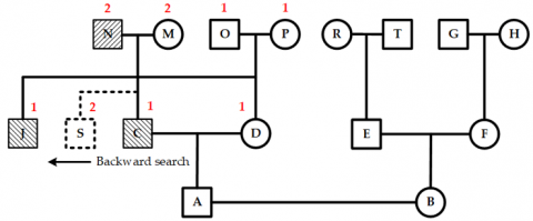
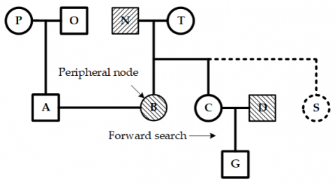
Peripheral nodes are those positioned at the outermost left or right edges of each layer within both the initial and ancestor node sets.
Forward and backward nodes are nodes located to the right and left of a specific node at the same layer. The node immediately next to the right (or left) of the current node is called the forward (or backward) adjacent node.
3.2 Region-based pedigree layout
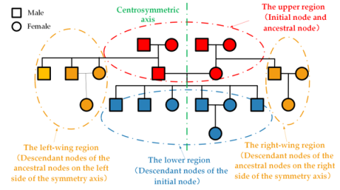
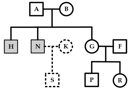
A pedigree layout is usually arranged symmetrically around the perpendicular bisector of the initial nodes. Depending on where the nodes are placed, the pedigree is divided into four parts: the upper, lower, left-wing, and right-wing regions (see Figure 1). The upper region includes the initial nodes and their ancestors; the lower region contains all their descendants; and the left-wing and right-wing regions represent the descendants of those ancestor nodes.
Figure 1. Pedigree region division
Node deletion in pedigrees is simple. If the node to be removed is in the lower or wing regions, its spouse and all descendants must also be removed. If the node is in the upper region, then all nodes from the top layer of the pedigree down to the layer containing the current node, along with their descendants, must be deleted.
Adding new nodes, unlike other modifications, often disrupts the structural balance of the pedigree layout, leading to a chain reaction of position adjustments for related ancestor or descendant nodes. This study focuses on creating and evaluating layout rules for node addition across different scenarios, aiming to preserve spatial coherence and visual clarity in dynamic pedigree building.
Any new nodes added must adhere to the existing pedigree layout rules. Their placement depends on whether they are a spouse, parent, or child, as well as the position of the current node.
4.1 Layout of spouse nodes
The spouse node remains on the same hierarchical layer as the current node and is positioned directly next to it in the forward horizontal direction. The layout is shown in Figure 2.
Figure 2. Layout of spouse nodes
4.2 Layout of parent nodes
Adding parent nodes to the pedigree must follow a strict hierarchy: only top-layer nodes can have parent nodes added. Spatially, these new parent nodes are placed one layer above the current node, classified as ancestors, and are fixed in the upper region of the pedigree.
Ancestor-type nodes in the upper region are built using a bottom-up recursive approach, starting from the topmost nodes and gradually adding parent nodes. These ancestor nodes are always depicted as spousal pairs, each consisting of two different individuals; therefore, the number of new ancestor nodes doubles with each step. Specifically, the number of parent nodes added is twice the number of nodes in the highest current layer, as shown in Figure 3. For example, beginning with two top nodes, adding their parents results in four ancestor-type nodes in the next layer, forming two spousal pairs.
Figure 3. Layout of parent nodes
4.3 Layout of child nodes
Child nodes are arranged in a strict hierarchy, with each node directly beneath its parent. Their placement primarily depends on two factors: (1) how nodes are distributed in the pedigree, and (2) the density and position of sibling nodes. These factors together shape the overall layout of child nodes. To better understand how child nodes are organized, the following discussion examines two key aspects: region distribution and the impact of sibling nodes.
4.3.1 Layout of child nodes in the lower region
When the current node already has one or more child nodes, it indicates that a matching spouse node exists. The rules for adding a new child are as follows: if the youngest child (the rightmost) does not have a spouse, the new child will be placed immediately after this node. If the youngest child does have a spouse, then the new child will be positioned after the spouse node. This layout arrangement for the second scenario is shown in Figure 4.
Figure 4. Layout of the youngest child with a spouse node of the current node
When the current node has no children, check for a spouse first. If there is no spouse, add one before proceeding with the other steps. Then, update the layout based on the context of the node addition.
(1) The current node has no backward node
If the current node has no backward nodes, the new child will be positioned at the leftmost spot on the next lower layer relative to it. Figure 5 shows the layout when the current node has no spouse or backward node.
Figure 5. Layout when the current node has no backward nodes
(2) The current node has backward nodes that lack children
If the current node has one or more backward nodes, but none of these nodes have children, the new child will be placed at the leftmost position on the next layer below the current node. Figure 6 illustrates the layout used when the current node does not have a spouse node and the backward nodes have no children.
Figure 6. Layout when the backward nodes of the current node have no children
(3) The current node has backward nodes with children
If the current node has one or more backward nodes and at least one of these has children, a backward search should be conducted. This process starts at the current node and moves backward along the same layer to find the nearest node with children. The placement of the new child depends on whether the youngest child of that backward node has a spouse. If a spouse exists, the new child is placed immediately after the spouse. If not, it is positioned after the youngest child. Figure 7 shows the layout when neither the current node nor the youngest child of its backward nodes has a spouse.
Figure 7. Layout of the youngest child node of a backward node without a spouse
4.3.2 Layout of child nodes in the wing regions
Child nodes in wing regions should be managed differently depending on the region of their parent node (i.e., the current node).
When the current node is identified as a non-ancestor, it is located within the wing regions of the pedigree. In such cases, the placement of new child nodes follows the layout described in “Layout of child nodes in the lower region”.
When the current node is an ancestor-type node, it appears in the upper region. Typically, it has at least one ancestor-type child, whose position does not indicate a specific birth order within the family. Any other children are considered second, third, or later children of this node. (Note: This explanation is for clarity and does not imply family birth order.)
Adding such nodes should not disrupt the existing pedigree layout. Applying rules from “Layout of child nodes in the lower region” directly may cause issues like misaligned nodes, intersecting connectors, or the lower region splitting into disconnected parts. These problems reduce visual clarity and waste space. To create a clean, attractive layout, specific placements are proposed for adding children to ancestor-type nodes in wing regions, as detailed in “Layout for children of ancestor-type nodes in wing regions”.
4.4 Layout for children of ancestor-type nodes in wing regions
To clarify the layout for adding children to ancestor-type nodes in the wing regions, a priority attribute is introduced to specify the relative positions of the ancestor-type nodes and their children in the pedigree.
4.4.1 Features of the priority attribute
The priority attribute has these four features:
Attribute inheritance. Only ancestor-type nodes have the priority attribute, while other node types do not. Children of ancestor-type nodes can inherit the priority value from their parent to maintain hierarchical consistency.
Spatial symmetry. Ancestor-type nodes are arranged symmetrically around the pedigree's centrosymmetric axis. Nodes on opposite sides have their priority values perfectly aligned, creating a balanced visual layout.
Distance correlation. The priority given to an ancestor-type node decreases as its distance from the symmetry axis increases. Nodes closer to the axis have lower priority values, while those farther away are assigned higher values.
Spousal priority consistency. Pairs of spouse nodes among ancestor-type nodes share the same priority values. This alignment maintains the spatial relationships between spouses and helps preserve the integrity of the overall pedigree layout.
Using the centrosymmetric axis as a reference, the spouse nodes immediately adjacent on each layer receive the lowest priority (baseline value = 1). The priority increases by 1 for each subsequent pair of spouse nodes symmetrically extending from the axis, establishing a clear priority order.
4.4.2 Priority-based layout of children
The placement of newly added children depends on their ancestors' priority and their of creation order. There is an inverse relationship between priority and distance from the centrosymmetric axis: higher-priority ancestors tend to have children closer to the axis, while lower-priority ancestors have children farther away. Additionally, the layout should consider the influence of sibling order. If an ancestor-type node in the wing region already has children, placing a new child depends on the youngest existing child (or their spouse, if present). If not, the new child's position depends on the youngest child (or their spouse) of its backward node.
(1) Layout of the second child of an ancestor-type node
When an ancestor node is on the left side of the centrosymmetric axis, its newly added second child is placed in the left-wing region. The layout process begins with a backward search from the leftmost node at the layer where the new child will be inserted. The final position of the new node is determined by this search, following specific layout rules as needed.
If the backward search finds no result, the new child will be placed at the leftmost position of its layer in the hierarchy, as shown in Figure 8.
If the backward search finds a node whose parent is not an ancestor-type node, it means the backward node is a regular node without a priority attribute. As a result, the new child will be placed immediately after this backward node in the forward direction. The layout is shown in Figure 9.
If a backward node is found during the search but no node with a lower priority than the new child exists, the new child will be placed at the leftmost position of the relevant hierarchy, as shown in Figure 10.
If the search finds the first backward node with lower priority than the new child, the new child will be inserted in the position immediately before this node. The layout is shown in Figure 11.
When an ancestor-type node is located on the right side of the centrosymmetric axis, the new child node will be placed in the right-wing region. The layout rules are similar to those for the left-wing region, but a forward search begins from the rightmost peripheral node at the layer where the new child is to be added.
Figure 8. No backward node detected
Figure 9. Backward node with a non-ancestor parent
Figure 10. Backward nodes detected with no lower-priority node found
Figure 11. The first backward node with lower priority
(2) Layout of third or subsequent child nodes of an ancestor-type node
When adding a third or later child to an ancestor-type node, it indicates that this node already has children in the wing region. The layout process starts by finding the node's youngest child. If that child has a spouse, the new child is placed behind the spouse on the left wing or in front of the spouse on the right wing. If there is no spouse, the new child is positioned behind the youngest child on the left or in front of the youngest child on the right. Figure 12 shows an example where a new child is added to the right region, with the youngest child having a spouse.
Figure 12. The youngest child node in the right-wing region has a spouse node
Placing a new node depends on the positions of nodes on the same and adjacent layers. Adding a node can trigger a ripple effect, causing other nodes to shift as well. Traditional top-down, left-to-right methods often require multiple repositioning steps. This is especially evident when organizing child nodes, resulting in cascading adjustments. As a result, this increases computational complexity and can cause a cluttered layout.
To address the issue above, a layout-based pre-allocation method for node placement is introduced using pedigree region division. It works hierarchically: starting with the top region, then the bottom, and finally the wings. Specifically, node locations in the upper region are assigned first, followed by those in the lower section, and finally, the nodes in the left and right wings. This regional approach reduces unnecessary position updates, enhancing computational efficiency and layout stability.
5.1 Position calculation of nodes in the upper region
Nodes in the upper region are organized hierarchically in a gradual manner. Starting from the top layer, ancestor nodes are positioned from bottom to top. After arranging each layer, a top-down adjustment is performed to ensure spouse nodes align with their children. This process continues until all nodes are properly arranged and aligned.
The detailed calculation process is as follows: first, node positions are assigned incrementally, starting from the initial nodes’ layer in a bottom-up manner. Within each layer, nodes are evenly spaced from left to right. The horizontal coordinate of each node is calculated as xPos=i*HUNIT, where i is the node’s index from the left. The vertical coordinate is given by yPos = RelativeY × VUNIT, where RelativeY indicates the layer’s relative distance from the initial layer. RelativeY is zero for the initial layer, decreases by one for each layer above, and increases by one for each layer below. VUNIT represents the vertical distance between layers. Next, starting from the current layer, the midline alignment of spouse nodes with their children is gradually adjusted from top to bottom. The midline of each spouse node should align vertically with the center of its child nodes, continuing until reaching the initial nodes’ layer.
After constructing the upper region, its node positions remain fixed. Any future changes to nodes in other parts of the pedigree will only affect the overall positioning of this upper region.
5.2 Position calculation of nodes in the lower region
The position calculation for nodes in the lower region starts with the layer that contains the children of the initial nodes. The midline of each spouse node should gradually align with the midlines of their respective children, including any spouses, which are evenly spaced at this layer. This step pre-allocated the positions of the children. Next, conflict detection is performed among these pre-allocated nodes. If overlaps are found, a separation adjustment is made, moving nodes within the conflict area together to eliminate overlaps.
(1) Node position pre-allocation
Starting from the layer immediately below the initial nodes, node positions are pre-assigned sequentially for each layer. Within each layer, nodes are evenly spaced from left to right, with their positions determined by their parent nodes. Specifically, the midline of parent nodes aligns with that of their evenly spaced children, including any spouses, ensuring accurate pre-allocation of child node positions.
The position of the first child node C is calculated as follows:
$\begin{gathered} {node}(C) \cdot x {Pos}=({node}(H) \cdot x {Pos}+{node}(W) \cdot x {Pos} -(K-1) * {HUNIT}) / 2\end{gathered}$
$node (C) \cdot y Pos =\binom{ {node}(C) \cdot{RelativeY}}{+ {node}({init}) \cdot { RowIndex}} * VUNIT$
where, H and W denote the spouse nodes, and K indicates the total number of children of the spouses H and W.
(2) Node conflict detection
The layer directly below the topmost node in the lower region does not cause position conflicts. However, as the hierarchy gets deeper, nodes in this region may encounter position conflicts during pre-allocation based on their parents' locations. For a node N with pre-allocated children positions, and its backward-adjacent node M, retrieve the positions of M’s youngest child node P (or its spouse, if any) and N’s oldest child node Q. Then, calculate the conflict value $v$ between nodes P and Q. If $v>0$, it indicates a position conflict that requires a layout adjustment.
(3) Layout adjustment based on the separation point
The primary objective of the layout adjustment is to prevent node overlaps by identifying the optimal separation point in the conflict area and shifting the entire conflicting area to the right. The detailed steps for this process are explained below.
(a) Identifying the separation point.
When a conflict occurs between adjacent nodes M and N at layer α, the first step is to check if their parent nodes—J on the left and K on the right—are the same. If they are different, J and K are recursively updated to their respective parent nodes (either the father or the mother) until the common parent U is found. Once this shared parent is identified, the midpoint between nodes J and K is marked as the separation point for resolving the conflict. The layer containing nodes J and K is called the separation layer, while the layer where the conflicting nodes M and N reside is known as the conflict layer.
(b) Identifying and relocating the conflict area.
The conflict area includes node K, all its child nodes (including spouse nodes) of U located to the right of K, and all their descendants. Moving this entire conflict area to the right by a distance of $v$ will resolve the conflict between nodes M and N.
If U is the initial node, the separation layer is directly below it. Moving the conflict area to the right in this case won’t cause secondary position conflicts. However, if U is not the initial node, such movement could introduce new conflicts, requiring secondary conflict detection to maintain the layout's stability and consistency.
(c) Secondary conflict detection
Secondary conflict detection involves identifying and resolving conflicts similar to the initial detection. However, their causes differ: the initial conflicts mainly result from the dynamic node drawing process, while secondary conflicts are primarily caused by layout adjustments. Both processes focus on locating conflict areas and making necessary adjustments.
Layer α conflicts are addressed in step (3). Afterward, secondary conflict detection focuses only on layers between α - 1 and the separation layer. The process begins from layer α - 1, and moves upward through the hierarchy until it reaches the separation layer. During this ascent, starting from node K at each layer, the system scans to the right to find node P and its adjacent node Q. If the parent nodes of P and Q (either father or mother) differ, it evaluates whether a positional conflict exists between them. When a conflict is identified, a corresponding conflict value is calculated. The layer with the highest conflict value among all is selected as the new separation layer, and the midline between nodes P and Q on this layer establishes the baseline for the subsequent separation. This process continues until all positional conflicts are resolved.
5.3 Position calculation of nodes in wing regions
When constructing nodes in the wing regions, it is important to keep the overall positions of nodes in the upper and lower regions unchanged. All nodes in the wing regions should be placed outside the upper and lower nodes, specifically on the left or right sides. This wing region includes both children of ancestor-type nodes and other descendants.
Child nodes of ancestor-type nodes are placed according to their parent node's priority. Nodes with higher-priority parents are closer to the central symmetry axis, while those with lower-priority parents are positioned farther from it. For other descendants of ancestor-type nodes, the layout rules from Section C. Layout of Child Nodes are applied. This ensures that the descendant nodes of the innermost children stay positioned at the innermost location.
(1) Pre-allocating positions for children of ancestor-type nodes
Starting from the initial layer of nodes, an upward scan progresses through each subsequent layer. At each layer, the peripheral nodes are identified to determine their positions. From these peripheral nodes, traversal extends in both directions to collect all nodes whose parents are of an ancestor type, creating an ordered sequence called cList. Positions are then assigned to each node in cList and their spouse nodes at fixed intervals of HUNIT, extending outward from the peripheral nodes. This method results in a spatial arrangement where the non-ancestor-type children of ancestor-type nodes are ordered from the central axis outward, based on the priority of their parent nodes.
(2) Pre-allocating positions for other descendants of ancestor-type nodes
For each node in the cList, if the node has children, align the midline between the node and its spouse with the midline of the evenly spaced children, including any spouses. Then, assign precise positions to each child and spouse based on this alignment.
(3) Conflict detection in wing regions
For each pair of spouse nodes in the cList sequence, if they are in the left-wing region, calculate the conflict value $v$ between the rightmost child node (including its spouse node if present) of the pair and its forward neighboring node. If they are in the right-wing region, calculate $v$ between the leftmost child node of the pair and its backward neighboring node. A conflict value $v$ greater than 0 indicates overlapping nodes, which require a layout adjustment.
(4) Conflict adjustment based on separation point in wing regions
The primary objective of adjusting the layout in the wing regions is to find the conflict separation point and move the entire conflicting area outward to avoid node overlaps. The process includes these steps:
(a) Determination of the separation point
When a conflict occurs between adjacent nodes M (outer side) and N (inner side) at layer α, the first step is to check whether their father nodes J and K (or mother) are the same or both are children of an ancestor-type node. If not, J and K are repeatedly updated to their respective fathers (or mothers). This process continues until J and K share the same parent U or both are children of an ancestor-type node. The layer containing J and K is called the separation layer, while the layer with M and N is called the conflict layer. In the left-wing region, the conflict separation point is defined as the midpoint between the node J (or its spouse, if any) and node K. In the right-wing region, it is the midpoint between the node K (or its spouse, if any) and node J.
(b) Identifying and moving the conflict area
In the left-wing region, the conflict area includes all child nodes of node U located to the left of node K, along with their spouses and descendants. Conversely, the right-wing region consists of node J, all children of U situated to the right of J, and any spouse nodes and their descendants. Moving the entire conflict area outward by a distance $v$ can resolve the conflict between nodes M and N.
In the left-wing region, if the oldest child of node U has no back-adjacent node, and in the right-wing region, if the youngest child of node U has no forward-adjacent node besides its spouse, this adjustment won’t cause new node conflicts. Otherwise, the movement might cause additional conflicts, requiring subsequent secondary conflict detection.
(c) Secondary conflict detection
Layout conflicts at layer α are resolved in step (4), so the secondary conflict detection only focuses on layers between α - 1 and the separation layer. The process starts from layer α - 1 and scans upward through the hierarchy until reaching the separation layer. At each layer, beginning from node J, a leftward scan in the left-wing region retrieves node P and its backward adjacent node Q; similarly, a rightward scan in the right-wing region retrieves node P and its forward adjacent node Q. Conflicts between nodes P and Q are then checked. If a conflict exists, the conflict value is calculated. The layer with the highest conflict value determines the node separation layer, and the midpoint between nodes P and Q at that layer is selected as the next separation point. This process continues until all conflicts are resolved.
Nodes in a pedigree are arranged according to their topological relationships, creating a logical coordinate system that remains independent of how the data is visualized. This logical system is inherently separate from the screen’s visualization coordinate system. To fit the entire pedigree within a limited viewing area, a spatial mapping mechanism should be used to convert between logical coordinates and screen coordinates.
When a new node is added, the layout updates automatically, and a redraw happens. Since the pedigree's scale changes with the number of nodes but the visualization area mostly stays the same size, a virtual grid–based adaptive fitting algorithm is used. This method ensures the pedigree fits well within the visible space by automatically choosing the best scale, balancing node clarity, interface layout consistency, and user visual comfort.
6.1 Identifying rows and columns in the pedigree
After completing the node position pre-allocation, all nodes in the pedigree are assigned specific coordinates and maintain fixed relative positions. The number of rows (N) and columns (M) in the pedigree can be calculated by referencing four key nodes: the topmost node, the bottommost node, the leftmost node, and the rightmost node. The formulas for these calculations are provided below.
$\begin{aligned} & { line} N= { downNode } . Y- { upNode } . Y+1 \\ & { col } M= { rightNode } . X- { leftNode } . X+1\end{aligned}$
6.2 Establishment of the adaptive scaling factor
A grid–based mapping method is introduced to accommodate pedigrees of different sizes. The visualization space, with width visW and height visH , is evenly divided into square grid cells based on the pedigree’s rows and columns. To improve computation performance, the grid side length is limited to a multiple of 8. Additionally, to maintain visualization clarity, a minimum grid size minSize is set to prevent nodes from becoming too small in larger pedigrees. Under these constraints, the grid side length gridLen is calculated as follows:
$gridLen = \begin{cases}\max \left({minSize},\left\lfloor\frac{\min \left\{\frac{v i s W}{{col} M}, \frac{v i s H}{{line} N}\right\}}{8}\right\rfloor \times 8\right), & \text { if } \min \left\{\frac{v i s W}{{col} M}, \frac{v i s H}{{line} N}\right\}>{minSize} \\ { minSize }, & \text { else }\end{cases}$
Each grid unit accurately records its linked node's position and maintains all topological connections. This virtual grid guarantees a one-to-one correspondence between pedigree nodes and grid units. The organized spatial arrangement enables efficient calculation of the optimal adaptive scaling factor for visualizing the pedigree within the display area.
6.3 Boundary detection
The drawing area acts as the main workspace for visualizing and rendering pedigree data. Meanwhile, the visible area shows the pedigree within a limited screen space, which is usually smaller than the drawing area. To improve user interaction, a center-alignment method is used to keep the centers of both the visible and drawing areas aligned.
Automatic boundary detection relies on the minimum grid size constraint. When the pedigree exceeds the drawing area’s boundaries (width drawW, height drawH), a dynamic boundary detection algorithm automatically enlarges the drawing area to keep all content visible. Additionally, if the pedigree extends beyond the visible boundaries, an intelligent scroll navigation feature activates automatically to ensure all nodes remain easily readable.
6.4 Node mapping with the virtual grid
The visible area is centered within the drawing space. Using the top-left corner of the drawing area as the coordinate origin, the origin coordinates of the visible area (gridStartX, gridStartY) can be calculated based on the drawing area’s dimensions and the grid unit parameters.
gridStartX = drawW / 2 - nodeColM / 2 * gridLen
gridStartY = drawH / 2 - nodeLineN / 2 * gridLen
To ensure accurate mapping of the pedigree onto the virtual grid, the mapping process should satisfy the following conditions:
leftNode.X = gridStartX, topNode.Y = gridStartY
A mapping array is created dynamically to connect each node to its respective grid cell during pedigree mapping onto the virtual grid. This virtual grid has a sparse layout, with each pedigree node assigned to a unique cell. Not all cells contain node data; some serve as placeholders to maintain proper spacing and the overall structure.
During user interaction, the system continuously tracks the cursor's position to identify the corresponding virtual grid unit, enabling quick access to the related node information within the pedigree.
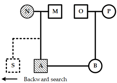
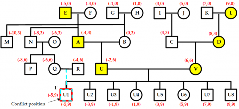
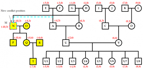
As shown in Figure 13, when a new child node T is added to the current node Q in the left-wing region, its position is pre-assigned based on its parent node Q’s location. This pre-allocation causes a position conflict between node T and node U1, with a conflict value equal to a two-unit distance.
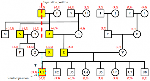
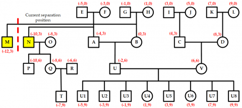
Since the parent node Q of T and the parent node U of U1 are different, and neither is a child of an ancestor-type node, it is necessary to move upward to the next hierarchical layer to identify nodes N and A. Because both N and A are children of an ancestor-type node, their shared layer is called the separation layer. At this point, the midpoint between node N's spouse node O and node A is the separation point for this conflict, as illustrated in Figure 14.
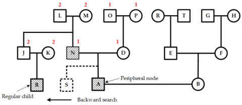
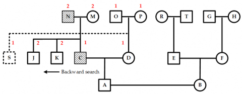
The nodes N and O, along with their descendant nodes P, Q, R, and T, form the conflict area. To resolve this, the entire conflict area shifts two units to the left, as shown in Figure 15. This movement causes a new conflict between nodes M and N, with a conflict value of two units. Because M and N are children of an ancestor-type node, their layer is again marked as the separation layer. At this point, only node M contains a new conflict area. To fix this, node M is shifted leftward by two units, completing the secondary conflict adjustment, as shown in Figure 16. Consequently, all conflicts in the pedigree are eliminated, and the pre-allocated positions for all nodes are finalized.
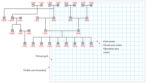
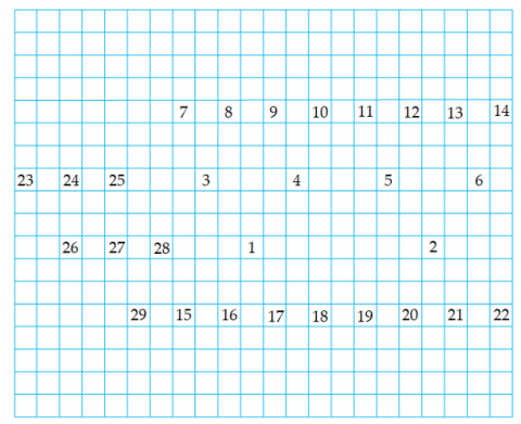
The pre-allocated pedigree might not be fully visible on the screen, as shown in Figure 17. To display the entire pedigree, a mapping between the pre-allocated pedigree and the visible area should be created. Based on the positions of node E(topmost layer), node T(bottommost layer), node M(leftmost layer), and node L(rightmost layer), the number of rows in the pedigree is calculated as nodeLineN=10, and the number of columns is nodeColM=22. Assuming a column spacing of 2 units and a row spacing of 3 units, with a visible area of width visW=1800 and height visH=1500, and a minimum virtual grid size of minSize=24, the grid side length gridLen is calculated as follows:
$gridLen =\max \left(24,\left\lfloor\frac{\min \left\{\frac{1800}{22}, \frac{1500}{10}\right\}}{8}\right\rfloor \times 8\right)=80$
Figure 13. Adding a new node to the left-wing region
Figure 14. Conflict detection in the left-wing region
Figure 15. Secondary conflict detection in the left-wing region
Figure 16. Secondary conflict adjustment in the left-wing region
Figure 17. Mapping pre-allocated node positions to the virtual grid
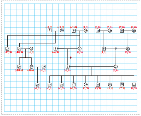
Figure 18. Pedigree visualization after position adjustment
Figure 19. Grid array for storing node identification
Reposition each node to keep the pedigree centered in the visible area, as shown in Figure 18. At the same time, create a grid array to store node identifiers, as depicted in Figure 19. This setup enables quick retrieval of node data using screen coordinates during user interactions.
The proposed automated pedigree layout algorithm uses virtual grids and region partitioning. It applies region-specific layout rules and develops strategies for node arrangement to depict pedigrees. The method generates a set of dynamic layouts for new nodes, employing different rules based on node types. Additionally, a priority-based layout approach for wing regions is introduced to enhance spatial efficiency. By utilizing virtual grids and node pre-allocation strategies, the algorithm improves layout performance and decreases computational load during dynamic updates. Through illustrative examples, the approach demonstrates its effectiveness in maintaining clarity, scalability, and interactivity in pedigree visualization. Future research will focus on real-time layout optimization for dynamic data updates and integrated visualization of complex family data.
[1] Bennett, R.L., French, K.S., Resta, R.G., Austin, J. (2022). Practice resource-focused revision: Standardized pedigree nomenclature update centered on sex and gender inclusivity: A practice resource of the National Society of genetic counselors. Journal of Genetic Counseling, 31(6): 1238-1248. https://doi.org/10.1002/jgc4.1621
[2] Miroševič, Š., Klemenc-Ketiš, Z., Peterlin, B. (2022). Family history tools for primary care: A systematic review. European Journal of General Practice, 28(1): 75-86. https://doi.org/10.1080/13814788.2022.2061457
[3] He, D., Wang, Z., Han, B., Parida, L., Eskin, E. (2013). IPED: Inheritance path-based pedigree reconstruction algorithm using genotype data. Journal of Computational Biology, 20(10): 780-791. https://doi.org/10.1089/cmb.2013.0080
[4] He, D., Eskin, E. (2014). IPED2X: A robust pedigree reconstruction algorithm for complicated pedigrees. Journal of Bioinformatics and Computational Biology, 12(6): 1442007. https://doi.org/10.1142/S0219720014420074
[5] He, D., Wang, Z., Parida, L., Eskin, E. (2014). IPED2: Inheritance path based pedigree reconstruction algorithm for complicated pedigrees. In Proceedings of the 5th ACM Conference on Bioinformatics, Computational Biology, and Health Informatics, California, pp. 202-210. https://doi.org/10.1145/2649387.2649438
[6] Mossel, E., Vulakh, D. (2022). Efficient reconstruction of stochastic pedigrees: Some steps from theory to practice. In Pacific Symposium on Biocomputing 2023: Kohala Coast, Hawaii, USA, pp. 133-144. https://doi.org/10.1142/9789811270611_0013
[7] Huang, X., Tatonetti, N., LaRow, K., Delgoffee, B., Mayer, J., Page, D., Hebbring, S.J. (2021). E-Pedigrees: A large-scale automatic family pedigree prediction application. Bioinformatics, 37(21): 3966-3968. https://doi.org/10.1093/bioinformatics/btab419
[8] Tokutomi, T., Fukushima, A., Yamamoto, K., Bansho, Y., Hachiya, T., Shimizu, A. (2017). f-treeGC: A questionnaire-based family tree-creation software for genetic counseling and genome cohort studies. BMC Medical Genetics, 18(1): 71. https://doi.org/10.1186/s12881-017-0433-4
[9] Guardado, M., Perez, C., Campana, S., Chavez Rojas, B., et al. (2025). py_ped_sim: A flexible forward pedigree and genetic simulator for complex family pedigree analysis. BMC Bioinformatics, 26(1): 122. https://doi.org/10.1186/s12859-025-06142-z
[10] Nieuwoudt, C., Brooks-Wilson, A., Graham, J. (2020). SimRVSequences: An R package to simulate genetic sequence data for pedigrees. Bioinformatics, 36(7): 2295-2297. https://doi.org/10.1093/bioinformatics/btz881
[11] Dimitromanolakis, A., Xu, J., Krol, A., Briollais, L. (2019). sim1000G: A user-friendly genetic variant simulator in R for unrelated individuals and family-based designs. BMC Bioinformatics, 20(1): 26. https://doi.org/10.1186/s12859-019-2611-1
[12] Kirkpatrick, B., Li, S.C., Karp, R.M., Halperin, E. (2011). Pedigree reconstruction using identity by descent. Journal of Computational Biology, 18(11): 1481-1493. https://doi.org/10.1089/cmb.2011.0156
[13] Dang, H.T., Tan, S.J.S., Mathieson, S. (2022). Comparison of cohort-based identical-by-descent (IBD) segment finding methods for endogamous populations. In Proceedings of the 13th ACM International Conference on Bioinformatics, Computational Biology and Health Informatics, Northbrook, Illinois, pp. 64. https://doi.org/10.1145/3535508.3545104
[14] Carver, T., Cunningham, A.P., Babb de Villiers, C., Lee, A., et al. (2018). pedigreejs: A web-based graphical pedigree editor. Bioinformatics, 34(6): 1069-1071. https://doi.org/10.1093/bioinformatics/btx705
[15] Schönberger, J., Steinhaus, R., Seelow, D. (2024). Drawing human pedigree charts with DrawPed. Nucleic Acids Research, 52(W1): W61-W64. https://doi.org/10.1093/nar/gkae336
[16] Sun, C., Xu, J., Tao, J., Dong, Y., et al. (2022). Mobile-Based and Self-Service Tool (iPed) to Collect, Manage, and Visualize Pedigree Data: Development Study. JMIR Formative Research, 6(6): e36914. https://doi.org/10.2196/36914
[17] Santos, J.M., Santos, B.S., Teixeira, L. (2015). Interactive clinical pedigree visualization using an open source pedigree drawing engine. In International Conference on Human-Computer Interaction, Los Angeles, CA, USA, pp. 405-414. https://doi.org/10.1007/978-3-319-20901-2_38
[18] Ranaweera, T., Makalic, E., Hopper, J.L., Bickerstaffe, A. (2018). An open-source, integrated pedigree data management and visualization tool for genetic epidemiology. International Journal of Epidemiology, 47(4): 1034-1039. https://doi.org/10.1093/ije/dyy049
[19] Tekman, M., Medlar, A., Mozere, M., Kleta, R., Stanescu, H. (2017). HaploForge: A comprehensive pedigree drawing and haplotype visualization web application. Bioinformatics, 33(24): 3871-3877. https://doi.org/10.1093/bioinformatics/btx510
[20] Velinder, M., Lee, D., Marth, G. (2020). ped_draw: Pedigree drawing with ease. BMC bioinformatics, 21(1): 569. https://doi.org/10.1186/s12859-020-03917-4
[21] Ullah, E., Aupetit, M., Das, A., Patil, A., et al. (2019). KinVis: A visualization tool to detect cryptic relatedness in genetic datasets. Bioinformatics, 35(15): 2683-2685. https://doi.org/10.1093/bioinformatics/bty1028
[22] Mäkinen, V.P., Parkkonen, M., Wessman, M., Groop, P.H., Kanninen, T., Kaski, K. (2005). High-throughput pedigree drawing. European Journal of Human Genetics, 13(8): 987-989. https://doi.org/10.1038/sj.ejhg.5201430
[23] Voorrips, R.E., Bink, M.C., van de Weg, W.E. (2012). Pedimap: Software for the visualization of genetic and phenotypic data in pedigrees. Journal of Heredity, 103(6): 903-907. https://doi.org/10.1093/jhered/ess060
[24] Bui, D.K., Jiang, Y., Wei, X., Ortube, M.C., Weeks, D.E., Conley, Y.P., Gorin, M.B. (2015). Genetic ME–a visualization application for merging and editing pedigrees for genetic studies. BMC Research Notes, 8(1): 241. https://doi.org/10.1186/s13104-015-1131-y
[25] Garcia-Giordano, L., Paraiso-Medina, S., Alonso-Calvo, R., Fernández-Martínez, F.J., Maojo, V. (2020). Genodraw: A web tool for developing pedigree diagrams using the standardized human pedigree nomenclature integrated with biomedical vocabularies. In AMIA Annual Symposium Proceedings, pp. 457-466.
[26] Razi, S., Gardner, H., Adcock, M. (2021). Immersive pedigree graph visualisations. In 2021 IEEE Conference on Virtual Reality and 3D User Interfaces Abstracts and Workshops (VRW), Lisbon, Portugal, pp. 659-660. https://doi.org/10.1109/VRW52623.2021.00212
[27] Carrizosa, C., Undlien, D.E., Vigeland, M.D. (2024). shinyseg: A web application for flexible cosegregation and sensitivity analysis. Bioinformatics, 40(5): btae201. https://doi.org/10.1093/bioinformatics/btae201
[28] Vigeland, M.D. (2022). QuickPed: An online tool for drawing pedigrees and analysing relatedness. BMC Bioinformatics, 23(1): 220. https://doi.org/10.1186/s12859-022-04759-y
[29] About Cyrillic 3. https://www.apbenson.com/about-cyrillic-3.
[30] Tang, D., Chen, M., Huang, X., Zhang, G., et al. (2023). SRplot: A free online platform for data visualization and graphing. PloS One, 18(11): e0294236. https://doi.org/10.1371/journal.pone.0294236
[31] Freeman, S.C., Kerby, C.R., Patel, A., Cooper, N.J., Quinn, T., Sutton, A.J. (2019). Development of an interactive web-based tool to conduct and interrogate meta-analysis of diagnostic test accuracy studies: MetaDTA. BMC Medical Research Methodology, 19(1): 81. https://doi.org/10.1186/s12874-019-0724-x