Dinesh Kumar Jayaraman Rajendiran*![]() | Ganesh Babu
| Ganesh Babu![]() | Deepa Sundararajan
| Deepa Sundararajan![]() | Nivetha Lokiraj
| Nivetha Lokiraj
© 2025 The authors. This article is published by IIETA and is licensed under the CC BY 4.0 license (http://creativecommons.org/licenses/by/4.0/).
OPEN ACCESS
The records acquired from Electrocardiogram (ECG) are extensively used to predict heart disease. Therefore, the ECG signal is considered essential for evaluating medical data. However, it turns out to be a preliminary device that facilitates the observation of patients' health information. The peak values are an essential peak for providing reliable health conditions. Tracing the ECG signals is treated as the least complex technique for automatic prediction. The VLSI advancements show a significant impact on biomedical signal processing. The advancements rely on the circuit's functionality at high speed and it is modelled to consume lesser power and area. Specifically, for ECG signal denoising, digital signals like IIR and FIR filters are adopted in most real-time applications where FIR is widely used compared to IIR filters due to the higher-order performance and stability. Consequently, this research is investigated in a suitable testing environment to measure the model performance to discover the most delicate steps to address the challenges in the ECG signals. The features obtained through wavelet transform are then redefined and used as input for the classification algorithm and compare and evaluate various assessment metrics, including accuracy, precision, recall, and F-measure, against other methodologies.
Electrocardiogram, FIR, IIR, coefficients, neural networks, wavelet transform and classification
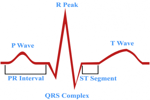
Generally, ECG is the process of electrical activity recording those outcomes with heart rate at a specific time frame. It is used to document information regarding structure of the heart that materializes triggered by depolarization of heart cardiac contractions synchronized with heartbeats [1, 2]. Also, it is composed of electrodes that are placed in various places over the individuals' skin. ECG signals are extensively utilized to predict heart illness, characterized by valleys and six peaks [3]. The valleys and peaks are generally labelled with $P, Q, R, S, T$, and $U$ symbols, as depicted in Figure 1. ECG signal is a bio-electrical non-stationary signal composed of essential clinical information [4]. In general, clinical data is based on the measurement of rhythm and rate of every single heartbeat, position and size of the heart chambers. Cardiac conduction system and pharmacological effects, occurrence of cardiac muscle cell presence and implanted pacemaker operational efficiency are the significant observations from the ECG signals [5]. Accurate ECG signal measurement is necessary carefully by the specialized cardiologists to predict the life-threatening arrhythmias [6]. However, the automatic cardiac disorder classification via the computerized analysis can offer diagnostic and objective outcomes and preserve both the cardiologists' effort and time. Nonetheless, the information pieces are exposed to damage by various kinds of noise, leading to a wandering baseline [7]. Subsequently, the wandering baseline leads to the repetition of indecorous screen patterns [8]. It happens to owe to the electrode malfunction like patients’ movement, bad minimizing electromagnetic interference with electrodes and inappropriate optimizing electrode sites with electronic device feedback and noise coupled from other electronic devices of high frequencies [9]. ECG signals also pose noise, changing waveforms that help observe inappropriate clinical measures and misleading factors. Therefore, the investigators have to adopt denoising algorithms for attaining the transparent ECG signal, which intends to enhance the signal-to-noise ratio [10, 11]. There are diverse techniques for removing noise from ECG signals in linear and non-linear contexts like a noise reduction and signal enhancement using median filters, advanced averaging, Fourier transforms, adaptive filters, and wavelet transforms [12, 13]. Subsequently, improving the processing algorithm to enhance the ECG signal quality is suggested. ECG denoising techniques also pose certain downsides as it avoids noise and eliminates high-frequency non-stationary signal components vital during waveform detection. Hence, the superior needs to produce a readily clear and observable signal that preserves the original waveform characteristic devoid of distortion. Recently, EMD has been initiated as an essential approach for non-linear and non-stationary signal processing. EMD serves as an alternative to those techniques. However, this EMD does not fulfil the requirements of specific real-time applications [14, 15].
Figure 1. Partition representations of ECG signal and segments
The existing model often misclassifies the signals with minor noises unless trained with a proper filtering process. The existing models turn to be biased towards the prediction of signals, with reduced sensitivity towards critical events like ventricular fibrillation. Some existing approaches are not suitable for real-time or edge devices with constrained processing power and battery life. The proposed NN, FIR and IIR filters perform distinct but complementary roles while dealing with ECG signal processing. The proposed filter models are adopted in pre-processing to improve the input signal to give quality outcomes and to eliminate artifacts or noise. The proposed FIR filter intends to preserve the waveform shape which is a complex task w.r.t ECG signals where morphologies like T, P, and QES waves are involved. The FIR filter model relies on the present and past inputs to maintain stability. Similarly, IIR filters needs lesser coefficients than FIR filters to enhance the performance. This filter considers both present and past inputs. These filters are employed to deal with real-time monitoring because of the lower computational cost. The proposed NN classifier is used for performing the higher-level processing tasks like feature extraction, classification and ECG signal interpretations. The proposed classifier model categorizes the beats as abnormal and normal, and predicts the T, QRS, and P wave boundaries. The classifier is capable of learning features from the partially noise data. The NN model helps in fine-tuning of individual variability. The novelty of the proposed model relies on the cleaning of raw ECG signals and helps in predicting the waveform components. The major research contributions are discussed below:
1.1 Research contributions
(1) This work describes the effectual computational approaches for analyzing and enhancing and offers a clear outline regarding the advancements of VLSI circuits over ECG signal processing. ECG signals are acquired from the available online resources, and the data source is composed of ECG signal data: testing and training data. The information is sourced from downloadable materials from the ECG MIT-BIH dataset.
(2) The dataset includes essential information regarding ECG signals, and it is used for further processing using the workspace in SIMULINK. The signals are denoised with the proposed improved IIR filter coefficients. The input consists of extracted features to the wavelet transform, and the effective classification is realized with the classifier model using neural networks.
(3) NN does not require any human intervention as it holds nested layers in passing the data via various conceptual hierarchies, which eventually has the competency of learning its own error. It can also handle an enormous volume of raw ECG signals by facilitating to deal of advanced data challenges. However, NN works well will provision more data. When compared to other learning approaches, the proposed NN reaches a higher level where huge samples do not influence the performance.
(4) The evaluate metrics like accuracy, precision, F-measure, and recall, we compare them against current techniques. The model strikes a better balance than the existing methods.
(5) Also, an ablation study if provided to examine various effects of signal processing components. The study helps to evaluate the combined and individual contributions using 1) NN without class imbalance and denoising; 2) NN without denoising; 3) NN with balanced class distribution; 4) NN with denoising, and 5) NN with class distribution skew. The model is designed to enhance the effectiveness of NN over ECG data.
The study is organized as follows: Section 2 presents a thorough examination of various methodologies modelled by the investigators. In section 3, the problem statement of the work is demonstrated and paves the way for further enhancements. The ECG signal enhancements are achieved with FIR and IIR filter designs and the analysis of the ECG signal interference. Then, feature extraction and classification are performed to attain better prediction accuracy.
Bae et al. [16] provide a detailed analysis of EMD-based filtering approaches. The investigators present diverse approaches for experimental purposes, and ECG signal classification is done effectually. These investigations involve pre-processing, feature extraction, and noise reduction and classification [17]. Researcher discusses three diverse denoising approaches: EMD-based noise reduction approaches, EMD-based partial reconstruction, and extracting inferences for adaptive filtering. Based on the changing noise amplitudes, these novel approaches intend to perform effective noise reduction methods provided ECG signal under a specific frequency ($48 \mathrm{~Hz}-51 \mathrm{~Hz}$). However, these approaches summarize the EMD enhancements method, which adopts the signal dependency property and is an adaptive technique [18]. Subsequently, these investigations show improved performance in diminishing removing noise with wavelets. This system's performance enhancement is generally coupled with two diverse conditions: a) there exist no constraints that the signal magnitude needs to be superior to the noisy signal, and b) lesser SNR [19-21] (Table 1).
Mukherjee and Ghosh [22] anticipate a novel approach for ECG signal improvement. This approach is based on the entire ensemble EMD with adaptive noise and higher-order statistical processing using mixed interval thresholds. Subsequently, the ECG signal is decomposed into the IMF components set with the EMD technique. IMFs attained are partitioned into three diverse groups: noiseless relevant, higher frequency noisy and lower frequency noise IMFs [23]. The novel derived criterion categorizes these approach groups based on the fourth-order cumulant. Therefore, the ECG signal is reconstructed by merging the threshold IMFs and reserved refined lower frequency appropriate IMFs. The author anticipates a new method for ECG denoising: DWT and EMD integration [24]. The anticipated performance of the windowing in Empirical Mode Decomposition to diminish the interference produced by the preliminary IMF is entirely avoided. However, the ECG signal attained varies in the DWT domain with the adaptive soft thresholding approach to diminish the noise [25]. However, the ECG signal is reconstructed in a superior time resolution of essential DWT properties evaluated to the EMD technique for energy conservation during the noise presence. Therefore, this work attempts to preserve the QRS complex to provide a clear ECG signal [26]. Martis et al. [27] utilized the EMD approach to enhance the noise filtering performance by reducing mode-mixing near the IMF's scales. However, the investigator performs experiments to model filtering ECG signals technique that relies focusing on lower IMF scales, including High-frequency noise. Comparing EEMD filtering performance and the existing EMD approach is highlighted in this work. Nonetheless, Wiener filter application is utilized to evaluate the filtering functionality with EEMD, which is another noise filtering approach. But the model fails to fulfil the requirements [28, 29]. This study concentrates on modelling a model for improving ECG signal accuracy by noise reduction using IIR and FIR filter comparison to handle these issues [30]. The ECG signal goes through several stages, including noise reduction, feature extraction, and classification, all aimed at enhancing prediction accuracy. This process allows for a comparison of the latest and most effective methods available.
Table 1. Comparative analysis of state-of-the-art methods for ECG filtering and prediction
|
References |
Dataset and Methods |
Approach |
Outcomes |
Constraints |
|
[16] |
AFIB dataset with SVM classifier model |
Gives a wider analysis of various existing learning approaches in healthcare applications. |
89.6% accuracy |
1) Only a certain piece of work was reviewed that which concentrates on ML applications on ECG signals based on heart disease classification. |
|
[19] |
AFL-203m dataset with ANN |
A novel deep learning framework is introduced for the detection and localization of myocardial infarctions using ECG data. |
92% accuracy |
1) No interpretability framework has been implemented for ML models in detecting myocardial infarctions. |
|
[20] |
MIT-BIH |
Offers a comprehensive evaluation of multiple deep learning techniques used for the prediction and classification of five distinct types of heart diseases from ECG signals. |
82% accuracy |
1) Covers interpretable models briefly and restrictively. |
|
[21] |
SPH and MLP classifier |
Highlights the importance and role of interpretability in deep learning models, particularly in healthcare-related applications. |
86% accuracy |
1) Emphasizes the role of feature relevance in explaining diverse machine learning models. 2) Presents a restricted evaluation of various interpretation approaches. |
|
[23] |
Linear SVM with MIT-BIH dataset |
Presents a concise yet informative overview of existing machine learning (ML) methodologies relevant to healthcare diagnostics. |
83% accuracy |
The analysis omits the use of interpretable models for heart disease classification from ECG data. |
|
[25] |
NSR samples |
Explores the key challenges in evaluating and implementing ML models, especially within real-world healthcare settings. |
90% accuracy |
Highlights how interpretable AI affects society at large Provides minimal insight into healthcare approaches, particularly those related to ECG-driven heart disease classification. |
|
[26] |
SVTA samples with TERMA |
Provides an in-depth discussion on the quality and reliability of machine learning approaches in clinical decision-making. |
37% accuracy |
Examines the application of ML methods in classifying heart disease from ECG data. |
This section outlines the problem statement related to the origin of the proposed model. This work concentrates on the prevailing FIR filter design constraints based on the broader literature study. However, various researchers recommended diverse variations and intended to provide the FIR filtering architecture. The advancements of the VLSI techniques give hope to making this architectural design an efficient one. This investigation intends to address various constraints of FIR filters along with the focus of the anticipated model to overcome the drawbacks of the prevailing FIR filters. Some general FIR filtering architectures are: 1) multipliers are consuming component. The multipliers are lesser efficient hardware than FIR filtering architecture with less effective design. 2) Also, adder design plays a substantial role in providing superior FIR filter architecture. 3) a productive pipelining process plays an effectual role in providing efficient FIR filter-based hardware. The solution is to address these constraints of FIR filter design using the IIR filters with the measure of coefficient values. The variables extracted from the IIF coefficients are provided as the input to the identifying key features process. Here, Wavelet decomposition-based feature extraction is done, and the most influencing features used as input to the classifier model, i.e., neural networks. Some essential metrics are computed to show the model's significance.
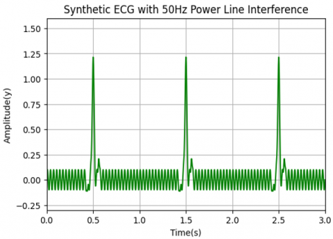
Various approaches are discussed for the noise removal process from the ECG signal. This work provides a broader analysis of the filters for low and high frequencies., i.e., FIR/IIR filters. The filtering approaches are commonly applied in signal processing and executed in diverse ECG signal analyses. However, filtering approaches improve the ECG signals, managed and implemented using FIR/IIR filters. Here, both these filters remove the noise over the ECG signals. Moreover, certain intrinsic noise agglutinant of the ECG signals is removed using the proposed approaches. However, ECG signal filtering is determined to be contextual. It is executed when the desired data remains ambiguous and needs further execution. However, the filtering process is considered an essential issue where the data needs to be disposed of and filtered. Later the denoised signals are provided to the feature extraction phase and map the wavelet based on time and frequency. It is determined to be technique for analyzing time-varying signals. The WT is appropriately utilized specifically for denoising as the wavelets show similarity with the energy spectrum, and QRS complexes are focused around low frequencies (See Figure 2). Finally, classification is done for prediction purposes.
Figure 2. The representation of synthetic ECG signal with interference (Power Line of 50 Hz)
4.1 FIR filter
The digital filters are analog-to-digital converters and perform the vice-versa process (digital-to-analog). The LTI filter produces the filter coefficients specify the designing filters using impulse response. The linear filter coefficients convolution with input sequences provides the output as in Eq. (1):
$Y=f * x$ (1)
Impulse response specified by function f, input signal is denoted by x, and output signal y resulting from convolution. Convolution of input signal with filter as in Eq. (2):
$\begin{gathered}Y[n]=x[n] * f[n] \\ =\sum_k x[k] f[n-k]=\sum_k f[k] x[n-k]\end{gathered}$ (2)
Here, $Y[n]$ specifies the filter output, $x[n]$ represents the digital input (filter), $f[k]$ specifies the impulse response, and * represents convolution operators. The summation is provided by $k$, representing the impulse response (filter). The filter with finite value is known as the FIR filter. The digital filter class with the current and historical input data and none of the prior filter output to attain the present output value is known as the FIR filter. It is termed as FIR filter implementation. FIR filter operation is the time-domain smoothing via moving average. The low-pass (FIR) with the window design approach is quite simple and produces the filter output with superior performance. The passband/stopband deviations are equal approximately. However, it is general to attain pass band deviation is extremely smaller than stop band deviation. These parameters are not controlled independently in the window design. This, it is essential to design the filter in the passband to fulfil the stopband requirements. The ripple is not uniform and diminishes when it moves away from the transition band. The filter shows features like the passband specification $\varphi_p$ frequency, $\omega_s$ stopband frequency and transfer function (desired). The filter class (special) that fulfils the criteria is the equi-ripple FIR filter. This design reduces the maximal deviation from the transfer function. It poses approximation error with weighting among the actual and desired filter response in passband and stopband regions to reduce the maximal error. Therefore, the outcome possesses a stopband and passband ripple specifications $\operatorname{Hd}(\omega)$ specifies the filters' frequency response, $w(\omega)$ defines the weighted frequency response characteristic. The designer can select the relative error size in diverse spectral bands. This is represented by Eq. (3).
$H(\omega)=e^{-j \omega(M-1) / 2} e^{j(p / 2) L} H^*(\omega)$ (3)
Approximating error with weighted approach can be visualized as:
$E(\omega)=W(\omega)\left[H_d(\omega)-H^*(\omega)\right]$ (4)
$E(\omega)=W(\omega)\left[H_d(\omega)-P(\omega) Q(\omega)\right]$ (5)
The $Q(w)$ represents the frequency function,
$E(\omega)=W(\omega) Q(\omega)\left[H_d(\omega) / Q(\omega)-P(\omega)\right]$ (6)
Therefore, the approximation predicts reducing maximal error through coefficient adjustment $E(\omega)$ measure. The approximation formula is provided in Eq. (7):
$|E(\omega)|=\min [\max |E(\omega)|]$ (7)
FIR filter coefficients are produced with SIMULINK tool. The filter response accuracy relies on the filter coefficients. The filter (ideal) needs the filter tap weights is not probable to execute over the hardware. The approach to handle this problem is coefficient round off. It reduces the hardware utilization, therefore diminishing the hardware utilization. The depreciation of filter coefficients influences the filter performance, specifically when the numbers of tabs are significantly higher.
4.2 Low-pass serial and parallel FIR
The architectural view of the serial FIR filter needs one multiplier, one adder, and one delaying unit. Therefore, it is a superior option when considering hardware efficiency. However, the FIR filter is done via the architecture, with reduced device throughput and slower performance. Similarly, the parallel FIR low-pass filter intends to parallel process data, rather than processing it. It provides superior throughput. All adders are associated with the prior adder output. The result is attained from the sum of adders output and output terminal. It provides the valid output, and the delay is affected by key delay factors. It is hugely greater than or equal to the product sum and accumulator delays pretends to handle the high necessary delay. Here, the adders are connected with the bran tree and add data-parallel indeed of serial. It is so advantageous evaluated to the prior design and it diminishes the Critical delay considerations for FIR filter.
4.3 Analysis with IIR filter
Recursive filter implementation where the output is not associated with prior input. However, it is related to the preceding output. Two diverse design approaches are based on the IIR filter: indirect and direct. It is used to model IIR filters by restricting the zero distribution and pole of the transfer function. Similarly, indirect technique is based on analog filter prototype model to calibrate every filter coefficient based on the requirements. Then, Analog filtering techniques are mapped from the $S \rightarrow Z$ analog domain via the Laplace transform via transforming from S-domain to Z-domain yields a digital filter for processing digital signals (Tables 2-4).
Table 2. FIR parameter
|
Filter Order |
Pass Band Edge Frequency (Hz) |
Maximal Pass Band Ripple (dB) |
Minimum Stop Band Attenuation (dB) |
|
2 |
0.4 |
2 |
3 |
Table 3. IIR filter parameters
|
Filter Order |
Pass Band Edge Frequency (Hz) |
Maximal Pass Band Ripple (dB) |
Minimum Stop Band Attenuation (dB) |
|
2 |
0.1 |
2 |
3 |
Table 4. HPF parameters
|
Filter Order |
Pass Band Edge Frequency (Hz) |
Maximal Pass Band Ripple (dB) |
Minimum Stop Band Attenuation (dB) |
|
2 |
0.4 |
3 |
2 |
By the frequency domain analysis relies on the present information gathered during capturing ECG signals, it is identified that noise significantly affects the signal on the attained ECG signal, i.e., Signal baseline shift caused set breathing frequency, as $0 \sim 1 \mathrm{~Hz}$. The successive noise influence over the ECG signals is power line interference due to $220 \mathrm{~V}, 50 / 60 \mathrm{~Hz}$ AC grid infrastructure. Two filters need to be constructed to avoid the noise interference across two frequency ranges. Filters out low-frequency noise 0 to 1 Hz baseline drift, and the filters out high frequencies, it suppresses roughly interference (50 Hz frequency). The digital angular frequency (Z-domain) is expressed as in Eq. (8):
$\Omega=\frac{1}{f_{a d}} * f_s * 2 \pi n, n=0,1,2, \ldots$ (8)
Here, $f_{a d}$ denotes the ADC sampling frequency, while $f_s$ represents the signal frequency. Frequency $f_c=50 / 60$ has to be avoided when $f_{a d}=480, \Omega_c \approx n \pi / 5(n=0,1, \ldots, 9)$. Then, Notches are designed at $\Omega_c \approx \mathrm{n} \pi / 5(\mathrm{n}=0,1, \ldots, 9)$ to reject $50 / 60 \mathrm{~Hz}$ interference. Additionally, the zeros need consideration in 0 Hz and $\frac{50}{60} \mathrm{~Hz}$ at the point $(1,0)$ in the complex plane. A zero and a pole are strategically placed at $(1,0)$ to prevent frequency overlap. Poles at the origin $(0,0)$ or on the real axis like $(1,0)$ can provide a stable transfer function. For stability, poles are typically placed within the unit circle in the transfer function, as shown in Eq. (9).
$\begin{gathered}\left(e^{j * 0}-e^{j \Omega}\right)\left(e^{\frac{1}{5} \pi j-e^{j \pi}}\right) \\ H(j \Omega) \frac{\left(e^{\frac{2}{5} \pi j-e^{j \pi}}\right) \cdots\left(e^{\frac{9}{5} \pi j-e^{j \pi}}\right)}{\left(e^{j 0}-e^{j \Omega}\right) e^{9 j \Omega}}=\frac{e^{10 * j \Omega}-1}{\left(e^{10 * j \Omega}\right) e^{e j \pi}}\end{gathered}$ (9)
Here, $z=e^{j \Omega}$. Then,
$H(z)=\frac{z^{10}-1}{z^{10}-z^9}=\frac{1-z^{-10}}{1-z^{-1}}=\frac{Y(N)}{X(N)}$ (10)
Increasing the filter order improves the low-pass filter's performance. Eq. (11) outlines the transfer function for a second-order low-pass digital filter.
$H(z)=\frac{\left(1-z^{-10}\right)^2}{\left(1-z^{-1}\right)^2}=\frac{1-2 z^{-10}+z^{-20}}{1-2 z^{-1}+z^{-2}}=\frac{Y(N)}{X(N)}$ (11)
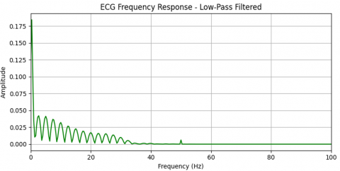
Magnitude-frequency characteristics of a low-pass filter is provided based on Eq. (11). Frequency characteristics attained from multiple filters are implemented using adding two filters with linear phase response and matched delay (See Figure 3(a) and Figure 3(b)), i.e., the weighted sum of filter coefficients. The high-frequency filter is modelled based on subtracting low-pass filter output from original signal. The signal filter poses a constant lag filter, expressed in $H a(z)=A z^{-m}$. Under specific ideal conditions, $H a(z), H_{o w}(z)$ poses a similar DC amplification coefficient. A filter that passes low frequencies is designed using threshold frequency of 2 Hz, i.e., $f_c=2 \mathrm{~Hz}$, when sampling rate is $f_{a d}=480$. The related radial frequency $\Omega c \approx n \pi / 120$, where ( $n=0,1,2, \ldots, 9$ ). Based on the integer filter design:
$H_{l p}(z)=\frac{Y(z)}{X(z)}=\frac{1-z^{-240}}{1-z^{-1}}$ (12)
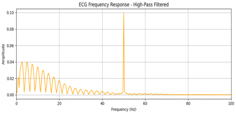
To create a high-pass filter obtained by subtracting low-pass from unity gain. The expression in Eq. (13) is this.
$H_{h p}\left(z^{\prime}\right)=\frac{P\left(z^{\prime}\right)}{X\left(z^{\prime}\right)}=z^{-120}-\frac{H_{l p}\left(z^{\prime}\right)}{240}$ (13)
$H_{h p}\left(z^{\prime}\right)=\frac{-1+240 z^{\prime-121}-240 z^{\prime-120}+z^{\prime-240}}{240-240 z^{\prime-1}}$ (14)
The response of the HPF under the frequency and magnitude curve is obtained from Eq. (14). The transfer function of the desired HPF is obtained using Eq. (15):
$H_{h p}(z)=\frac{P(z)}{X(z)}=z^{-120}-\frac{H_{l p}(z)}{240}$ (15)
(a)
(b)
Figure 3. (a) Amplitude-frequency response of low-pass filter; (b) Amplitude-frequency response of high-pass filter
Eq. (16) presents the differential form in detail:
$\begin{gathered}y(n)=2 * y(n-1)-y(n-2)+x(n)-2 \\ * x(n-10)+x(n-20)\end{gathered}$ (16)
The high-pass filter's transfer function is given in Eq. (17).
$\begin{gathered}y(n)=y(n=120) \\ -\frac{(y(n-1)+x(n)-y(n-240))}{240}\end{gathered}$ (17)
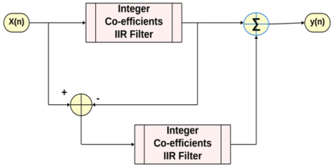
Generally, ECG signals show slight distortion after the essential process after the IIR filter (integer coefficients). Therefore, the coefficients are modelled to attain an entire ECG signal where the coefficients filter necessary information. An enhanced filter coefficient is proposed to achieve the essential information. Figure 4 depicts the structural design of every a dual-mode IIR filter module supporting both low-pass and high-pass filtering. Then, ECG signals are filtered using IIR filters with integer coefficients, and the original signal subtracts the processed signal and attains difference signals. The filter coefficients need to achieve the compensation signal. The signal needs to avoid the interference and preserves the essential information (features). The ultimate process is the construction of the waveform and the compensation signals are added after the filtering process to attain the final signal outcome (See Figure 4). Extract relevant features from the processed signal where wavelet transform is best suited.
Figure 4. Improved IIR filter (integer coefficients) block diagram
Generally, a wavelet specification a small function representation using wavelets $x(t)$ to the time-scale representation, and $x(m, n)$ represents it. The wavelet offers frequency and time domain information regarding the signal representation, and it is a much appropriate for non-stationary signals. When the wavelet transform poses diverse window sizes, narrow at high and broader the low frequencies; therefore, it is appropriate for entire frequency ranges. The actual wavelet application is competent in computing and manipulating data termed features. The multi-scale WTis decomposed as a signal to diverse scales. In general, WTis a wavelet convolution with $x(t)$ and expressed as Eq. (18):
$T_{m, n}=\int_{-\infty}^{+\infty} x(t) \Psi_{m, n}(t) d t$ (18)
By opting for an orthogonal wavelet basis $\Psi_{m, n}(t)$ the original signal can be precisely specified, which is reconstructed. The signal's approximation coefficient is given by Eq. (19).
$S_{m, n}=\int_{-\infty}^{+\infty}(a t) \emptyset_{m, n}(t) d t$ (19)
where, $m$ and $n$ the wavelet transform specifies amplitude scaling and translation. A discrete-time signal smoothing is represented by Eq. (20).
$x_0(t)=x_M(t) \sum_{m=1}^M d_m(t)$ (20)
where the signal smoothing (mean) at scale 'm' is specified by Eq. (21).
$x_M(t)=S_{M, n} \emptyset_{M, n}(t)$ (21)
The signal smoothing, tied to scale 'm' for a finite-length signal, is given by Eq. (22):
$d_m(t)=\sum_{n=0}^{M-m} T_{m, n} \Psi_{m, n}(t)$ (22)
The signal smoothing at a given scale combines approximations from finer scales. It is expressed as Eq. (23):
$x_m(t)=x_{m-1}(t)-d_m(t)$ (23)
In the wavelet transform (multi-resolution), original signal is provided via the low and high-pass filter and acquires detailed and approximated signal coefficients. The details represent high-frequency components; High-frequency components are captured at low scales, whereas low-frequency components are represented at high scales components and approximations. The diverse frequency bands are analyzed where the signal is broken down into detail coefficients and approximation coefficients. The original Wavelet evaluation in wavelet transforms extremely an essential task in choosing the specific wavelet function, i.e., no universal technique exists. It depends on the signal type needs to be examined. The signal is like a wavelet function is generally chosen as in Table 5. The wavelet transform is appropriately utilized specifically for denoising as the wavelets show similarity with the energy spectrum, and QRS complexes are focused around low frequencies.
During optimization, adopt synthetic and real ECG signals with known noise profiles and apply filters for accessing signal preservation and noise suppression. Some metrics like SNR, error, amplitude and duration can be optimized. The proposed wavelet transforms based feature extraction is adopted for analyzing features like QRS complex, RR intervals, P and T wave boundaries, R-peak location can be predicted appropriately with the proposed wavelet coefficients. Wavelets may suppress noise while maintaining sharp transitions and works efficient for predicting fast changing features like QRS complex. The proposed model helps in the appropriate prediction of certain ECG features like P wave, QRS complex and T wave. The model improves the diagnostic accuracy by acquiring the appropriate morphological details. The proposed feature extraction model reduces false positive and false negatives during the classification tasks. The proposed model facilitates multi-faceted analysis enabling superior feature sets for diagnostic models.
Table 5. Parameter specifications
|
Parameters |
FIR Filter |
IIR Filter |
|
Cut-off frequency |
Based on ECG frequency band |
Similar as FIR |
|
Filter order |
100 – 200 (high) |
2 – 8 (low) |
|
Phase response |
No distortion |
Distortion |
|
Delay |
Higher |
Lower |
|
Stability |
Stable |
Has to be validated |
The neural network (NN) comprises many neurons connected to transfer and receive the data concurrently. Every neuron in the network is allocated with the weight. It represents the network state during the learning process, and the weight of every neuron needs to be updated. The anticipated model of every neuron is completely connected to hidden layers for extracting features and categorizing the ECG signal. It is executed in SIMULINK, and the generalized sparse network model is adopted to diminish the number of features and enhance computational time. The feature extraction shows diverse descriptive parameters and data using the preliminary process from the ECG signals. The network model is trained and classified based on the feature vectors (features extracted using wavelet transform). During the analysis step, and double-check that the model still delivers quick, accurate results. At this point the module lays out its prediction work using a simple neural network pattern.
Cascaded neural network architecture are displayed by the fake neurons. The sources (features) B1,…,Bn are thought to be unidirectional and produce a sign stream of neurons. Eq. (24) provides the neuron output:
$o=f($network$)=f\left(\sum_{i=1}^n A_i B_i\right)$ (24)
The capacity is given as f(network), and the weighted vector is indicated by AiBi. the network. The variable network is represented as scalar consequences by the weight and information vectors. It is stated in Eq. (25):
network $=A^T B=A_1 B_1+A_2 B_2+\cdots+A_n B_n$ (25)
where, $T$ specifies the matrix transposition. The value of $O$ is given by Eq. (26).
$O=f($network$)=\left\{\begin{array}{lc}1 & \text { if } A^T x \geq \theta \\ 0 & \text { otherwise }\end{array}\right.$ (26)
Note that the model sets a fixed range as its ceiling, and a linear threshold unit (LTU) is a type of node. The neurons inside this scheme behave according to the equation shown in Eq. (27):
$v_k=\sum_{i=1}^p A_{k i} B_i$ (27)
Then, the neuron output $y_k$ is the outcome of the activation function of $v_k$. The error reduction among the evaluated EEG class is essential. The network performance is evaluated using the output (expected) with the raw output value. The proposed system is faster, and the data needs to increase forward like back-propagation NN, where the information is provided to forward and reverse a blunder. The relapse performed by the classifier is inevitable with the desire for $Y$ with the provided $X=a$. It gives the scalar value representing the input vector $a$. Let $f(a, b)$ illustrate vector irregular variable capacity $X$ and scalar arbitrary variable $Y$. The $a$ is provided with the chance to evaluate the stochastic estimation. The relapse variable Y is defined, with a restricted mean given by Eq. (28):
$E\left[\frac{Y}{X}\right]=\int_{\infty}^{\infty} Y, f\left(\frac{b}{a}\right) d y=\frac{\int_{\infty}^{\infty} Y, f(a, Y) d y}{\int_{\infty}^{\infty} f(a, Y) d y}$ (28)
In this context, X and Y point to the squeezed components, each set with its own chosen settings. The key link between a and b relies on non-parametric estimation done from scratch, so no advance knowledge is used.
6.1 Loss function
Assume N pair of training sample dataset:
$D=\left\{\left(a_s, b_s\right) \mid s=1, \ldots, N\right\}$ (29)
Here, $s$ indexes a single data point, $X_s$ stands for the input in $R^n$, and $Y_s$ in R records the corresponding output $a_s$. The goal is to estimate the hidden rule so that the prediction for every training pair stays within an accuracy band of size epsilon, while also uncovering how the outputs $a_s$ and $b_s$ relate to one another. That task starts by pushing all samples through a high-dimensional kernel map $\varphi: \mathrm{R}^{\mathrm{n}} \rightarrow \mathrm{R}^{\mathrm{m}}$, after which fit a simple linear model as shown in Eq. (30):
$f(a)=w^T \varphi(a)+c$ (30)
where, $w \in R^m$ the weighted vector, with 'c' indicating the threshold parameter. Here, 'w' stands for the minimal Euclidean distance, similar to described in Eq. (31):
$w=||w||_2^2$ (31)
The $\epsilon$ pair for precision representation is outlined in Eq. (31), which helps to reduce the error between the target output vs predicted output. To optimize the loss function, we express it as shown in Eq. (32):
$L\left(e_s\right)_\epsilon=L\left(b_s-f\left(a_s\right)\right)_\epsilon$ (32)
The proposed neural network optimization problem is shown below:
$J(w, c)=\frac{1}{2}| | w| |_2^2+P \sum_{s=1}^N L\left(b_s-f\left(a_s\right)\right)_\epsilon$ (33)
In this context, $P \in R^{+}$refers to parameters defined by the user. The level of noise present in the training samples is mentioned, but it doesn't factor into the output. As a result, the loss function, which is based on the optimization method, is designed to be sparse in order to find the solution.
$\left|b_s-f\left(a_s\right)\right|_\epsilon=\left\{\begin{array}{cc}0 & \left|b_s-f\left(a_s\right)\right|<\epsilon \\ \left|b_s-f\left(a_s\right)\right|-\epsilon & \text { else }\end{array}\right.$ (34)
From the statistical analysis, we've determined that the loss function is indeed optimal. Taking into account the error distribution, present the insensitive loss function as shown in Eq. (35): Please remember that when crafting responses, it's important to stick to the specified language and avoid using any others.
$L\left(e_s\right)_e=\left(e_s\right)_e^2$ (35)
In this context, $\left(e_s\right)_e^2$ represents a continuous differential function. By integrating Eq. (34) and Eq. (35), express the network model as shown in Eq. (36).
$\begin{aligned} w \in R^m, & b R^{J(w, c)}=\frac{1}{2} w_2^2+P \sum_{s=1}^N\left[\left(b_s-f\left(a_s\right)\right)\right]_\epsilon^2 \\ & =\left\{\begin{array}{c}b_s-w^T \varphi\left(a_s\right)-c \leq \varepsilon+\xi_s \\ -y_s+w^T \varphi\left(a_s\right)+c \leq \varepsilon+\xi_s \\ \xi_s, \xi_s^{\prime} \geq 0, s \in\{1, \ldots, N\}\end{array}\right.\end{aligned}$ (36)
Here, $\xi_s$ and $\xi_s{ }^{\prime}$ are the slack variables used to account for both negative and positive deviations. To calculate the primal objective of Eq. (37), we take the linear regression and multiply it by a non-negative multiplier for each sample set.
$\begin{aligned} w \in R^m, b \in R^{j\left(w, c, \alpha_s, \alpha_{s^{\prime}}^{\prime}, \gamma_s, \gamma_{s^{\prime}}^{\prime}, \xi_{s^{\prime}}, \xi_s^{\prime}\right)} =w, c, \alpha_{s^{\prime}}, \alpha_{s^{\prime}}^{\prime}, \gamma_s, \gamma_{s^{\prime}}^{\prime}, \xi_{s^{\prime}}, \xi_s^{\prime} \geq 0 s \in\{1, \ldots, N\}\end{aligned}$ (37)
$\begin{gathered}\frac{1}{2} w^T w+P \sum_{s=1}^N\left[\left(\xi_s\right)^2+\left(\xi_s^{\prime}\right)^2\right]-\sum_{s=1}^N \alpha_s\left(\varepsilon+\xi_s-\right. \\ \left.b_s+w^T \varphi\left(a_s\right)+c\right)-\sum_{s=1}^N \alpha_s^{\prime}\left(\varepsilon-\xi_s^{\prime}-b_s+\right. \\ \left.w^T \varphi\left(a_s\right)-c\right)-\sum_{s=1}^N\left(\gamma_s \xi_s+\gamma_s^{\prime} \xi_s^{\prime}\right)\end{gathered}$ (38)
Here, $\alpha_s, \alpha\left(s^{\prime}\right), \gamma_s$, and $\gamma_s{ }^{\prime}$ represent the Lagrange multipliers. To pinpoint the best solution, we need to get rid of the primal variable. Consequently, the partial derivative will equal zero.
$\frac{\delta J}{\delta c}=\sum_{s=1}^N\left(\alpha_s^{\prime}-\alpha_s\right)=0$ (39)
$\nabla_w J=w-\sum_{s=1}^N\left(\alpha_s-\alpha_s^{\prime}\right) \varphi\left(a_s\right)=0$ (40)
$\frac{\delta J}{\delta \xi_s}=P\left(2 \xi_s\right)-\alpha_s-\gamma_s=0$ (41)
$\frac{\delta J}{\delta \xi_s}=P\left(2 \xi_s^{\prime}\right)-\alpha_s^{\prime}-\gamma_s^{\prime}=0$ (42)
Substitute Eq. (41) and Eq. (42) in Eq. (43), the model handles optimization problem:
$\begin{gathered}\max _{\propto \in R^N} J\left(\alpha_s \alpha_s^{\prime}\right)=-\frac{1}{2} \sum_{s=1}^N \sum_{\gamma=1}^N\left(\alpha_s-\alpha_s^{\prime}\right)- \\ \left(\alpha_s-\alpha_s^{\prime}\right) \\ \varepsilon \sum_{s=1}^N+\sum_{s=1}^N b_s\left(\alpha_s-\alpha_s^{\prime}\right)-\frac{1}{2 P} \sum_{s=1}^N\left[\left(\alpha_s\right)^2+\left(\alpha_s^{\prime 2}\right)\right]\end{gathered}$ (43)
$\sum_{s=0}^N\left(\alpha_s^{\prime}-\alpha_s\right)=0$ and $\alpha_s^{\prime} \alpha_s \varepsilon[0, \infty]$ (44)
K refers to the kernel matrix, and the kernel function K(as, ar) is essentially the product of two samples, φ(as) and φ(ar).
$\left.K=\left[K\left(a_s, a_r\right)\right]_{s, r}=\left[\varphi^T\left(a_s\right) \cdot \varphi\left(a_r\right)_{s, r}\right]\right]$ (45)
The dual optimization problem tackles quadratic challenges that lead to distinct outcomes and minima, and find the optimal model and decision function for the test set samples detailed in Eq. (46).
$w=\sum_{a_s \in D V}\left(\alpha_s-\alpha_s^{\prime}\right) \varphi\left(a_s\right)$ (46)
$f(a)=\sum_{a_s \in S V}\left(\alpha_s-\alpha_s^{\prime}\right) k\left(a_s, a\right)+c$ (47)
From Eq. (47), evaluate the operation by applying the kernel function to the input space along with the training set samples, transforming them into a high-dimensional space. In this context, SV refers to the training set samples where $\alpha \_\mathrm{s}-\alpha \_\mathrm{s}^{\prime}$ $\neq 0$, and can skip evaluating $f(a)$ and $w$. This approach helps reduce computational time, allowing the model to focus on solving the problem at hand.
Based on a variety of literature analyses, calculate metrics such as accuracy, precision, specificity, recall, and error rate from the classifier's output. The simulation takes place in SIMULINK, and the experimental results show that its performance outshines many other methods. Below, the definitions and expressions for all these metrics. For every test fold in the dataset, make sure to collect the results, which should include True Positive (TP), True Negative (TN), False Positive (FP), and False Negative (FN).
TP: heartbeats are identified correctly;
FN: beats inaccurately identified;
TN: beats correctly identified as negative.
Precision $=\frac{T P}{T P+F N}$ (48)
Recall $=\frac{T P}{T P+F N}$ (49)
$F 1=\frac{2 * T P}{(2 * T P+F N+F P)}$ (50)
$R M S E=\sqrt{\frac{1}{N} \sum_{s=1}^N\left(b_s-f\left(a_s\right)\right)^2}$ (51)
This work extracted a feature (e.g., RR interval) from the MIT-BIH dataset for two rhythm classes: 1) Class A: Normal Sinus Rhythm (NSR) and 2) Class B: Premature Ventricular Contraction (PVC).
The Null Hypothesis H0 states that there is no meaningful difference in the RR interval when comparing Normal Sinus Rhythm (NSR) to Premature Ventricular Contractions (PVC).
Alternative Hypothesis (H1): A significant difference exists.
Thus, choose a statistical test: If data is normally distributed: use independent t-test.
If not normal: use Mann–Whitney U test (non-parametric).
Interpretation.
If p < 0.05, reject the null hypothesis ⇒ Significant difference.
If p ≥ 0.05, fail to reject ⇒ No significant difference.
However, the p-value is 0.01, which is significant for the proposed model.
7.1 Ablation study
In this section, dive into ablation research to see how different parts of the proposed model influence the results get. We're particularly looking at the data imbalance issues that pop up in the ECG dataset we're working with. We've tested a variety of outcomes under these conditions: 1) a neural network (NN) without class imbalance and denoising; 2) a NN without denoising; 3) a NN without class imbalance; 4) a NN with denoising; and 5) a NN with class imbalance.
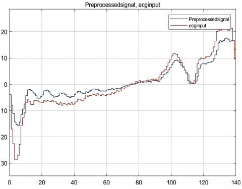
Figure 5. Pre-processed ECG signal
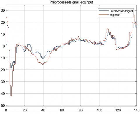
Figure 6. Pre-processed ECG signal
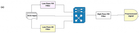
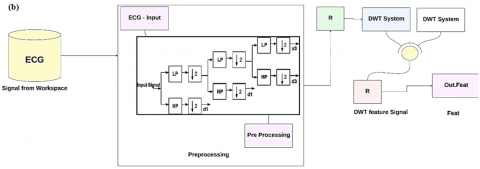
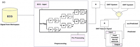
Figure 7. (a) Block diagram illustrating the pre-processing of ECG signals, including filtering stages; (b) Training model incorporating preprocessing and Discrete Wavelet Transform (DWT) for feature extraction; (c) Testing model employing the same preprocessing and DWT pipeline followed by a feed-forward neural network for classification
Table 6. A predicted table constructed based on ECG signal classification and comparative results with state of art existing methods
|
State of Art Methods |
Accuracy |
Precision |
Recall |
F1-score |
Error Rate |
|
GSNN [31] |
89 |
90 |
89 |
89 |
0.1568 |
|
ANN [32] |
87 |
88 |
68 |
69 |
0.2546 |
|
SVM (linear) [25] |
69 |
70 |
59 |
60 |
0.3564 |
|
SVM (Rbf) [25] |
68 |
70 |
60 |
65 |
0.1856 |
|
Proposed NN with wavelet transform and FIR/IIR filters |
92.3 |
73.4 |
98.5 |
90.6 |
0.0761 |
Table 7. Ablation study based analysis
|
Experiments |
Denoising Performed |
Class Imbalance Handled |
Functionality |
|
1 |
No |
No |
No pre-processing |
|
2 |
No |
Yes |
To evaluate the consequences of dealing with class imbalance alone |
|
3 |
Yes |
No |
To evaluate the consequences of dealing with denoising alone |
|
4 |
Yes |
Yes |
Complete mode with superior enhancements |
|
5 |
Yes |
Yes |
Test diverse class balancing strategies |
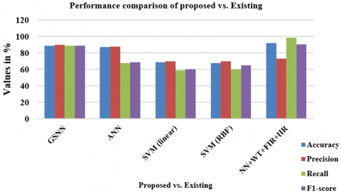
Figure 8. Performance comparison
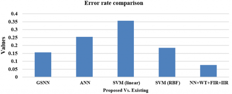
Figure 9. Error rate comparison
The results, based on the ECG dataset shown in Table 6, reveal that the model, which cleverly combines class imbalance handling and denoising, outperforms the others. When remove just one of these components, the performance of the other models takes a hit. This really underscores how important it is to use class imbalance strategies alongside denoising and balancing techniques. If take away two components, the performance of the model drops even further, highlighting just how crucial these elements are. This analysis emphasizes the importance of each component, their individual contributions, and how they work together to achieve the best results in predicting diseases from ECG data.
The provided raw ECG dataset is pre-processed with high-speed filters. Feature extraction and classification based on diverse methods are attained from the ECG dataset composed of sub-classes (See Figures 5-7). After completing all the preliminary steps, the neural network model uses various ECG features to evaluate the signal patterns and classifies those signals to predict cardiac issues. The proposed model also investigates the error rate, which is substantially lesser than other approaches. Table 6 and Table 7 depict the comparative analysis of the anticipated model with diverse approaches for ECG-signal based prediction and ablation study (See Figure 8 and Figure 9). The key metrics we’re looking at are accuracy, precision, recall, F1-score, and error rate. The expected accuracy of the new neural network (NN) is 92.3%, which is an impressive 3.3%, 5.3%, 23.3%, and 24.3% better than the GSNN, ANN, SVM (linear), and SVM (Rbf) models [31-35]. When it comes to precision, the anticipated model scores 73.4%, which is lower than both GSNN and ANN but still outperforms the SVM models (both linear and Rbf). As for recall, the proposed NN shines with a score of 98.5%, surpassing the other methods by 9.5%, 30.5%, 39.5%, and 38.5%. The F1-score of the anticipated model is 90.6% which is 1.6%, 21.6%, 24.6% and 25.6% higher than others. While the error rate is substantially lesser, i.e., 0.0761, which is lesser than other approaches, based on these metrics, it is proven that the pre-processing filters work effectually for denoising and give superior outcomes during the prediction process. NN does not requires any human intervention as it holds nested layers in passing the data via various conceptual hierarchies which eventually has the competency of learning its own error. It can also handle enormous volume of raw ECG signals by facilitating to deal with advanced data challenges. However, NN works well will provision more data. When compared to other learning approaches, the proposed NN reaches higher level where huge samples do not influence the performance. The NN models have the competency to learn themselves and offer the output which is not constraint to input provided to them. Also, the NN model shows fault tolerance as it pose the ability to respond to smaller changes in input and do not cause any output change normally.
It is well recognized that the MIT-BIH database includes ECG recordings from only 48 individuals, which presents a limitation in terms of data volume—an essential factor for effective NN based learning model training. To address this, the proposed algorithms were additionally evaluated on the more comprehensive MIT-BIH database which offers signals sampled at 360 Hz, the SPH dataset features a higher sampling rate of 500 Hz. The dataset is organized into four main directories: raw ECG recordings, denoised ECG data, diagnostic labels, and patient attributes. It encompasses a wide range of cardiac conditions, including 11 prevalent rhythms and 67 other cardiovascular abnormalities. Each of the 12 leads records a 10-second segment, resulting in 5,000 samples per lead. To keep things straightforward, organized the 11 types of rhythms into four main categories: SB, AFIB, GSVT, and SR. The SB category focuses on sinus bradycardia. The AFIB group encompasses both atrial fibrillation and atrial flutter. In the GSVT category, come across supraventricular tachycardia, atrial tachycardia, atrioventricular nodal re-entrant tachycardia, atrioventricular re-entrant tachycardia, and atrial wandering rhythm. Lastly, the SR group includes sinus rhythm and sinus irregularity.
7.2 Complexity analysis
A comparison of the computational complexity involved in both classifiers utilize feature extractions is presented. The complexity of computing the feature coefficients is expressed as $O\left(p^3\right)+O\left(p^2 N\right)$, whereas the discrete wavelet transform (DWT) has a computational complexity of $O(L N)$, Here, L represents the number of decomposition levels, and N denotes the number of samples per heartbeat. The symbol $\alpha$ is used to denote the computational cost associated with detecting Rpeaks. In the suggested method, R-peak detection is performed using the wavelet transform, which has a computational complexity of $O\left(N \log _2 N\right)$. In contrast, the approach used by Lai et al. [35] employed annotated R-peaks rather than estimated ones, resulting in a computation cost denoted as $\eta$, which varies depending on the algorithm used, assuming equal computational cost. for R-peak detection in both approaches, the classifier demonstrates a lower overall computational complexity, specifically by eliminating the $O\left(p^3\right)+O\left(p^2 N\right)$ overhead associated with model-based methods. The table also includes variations that incorporate additional features, highlighting the corresponding trade-offs between classification accuracy and computational cost. Among the features evaluated, PR interval, RT interval, age, and sex consistently emerged as the most effective in balancing accuracy and efficiency across different datasets.
The prediction model needs to operate quickly while using minimal power for real-time monitoring systems based on modern wearable ECG technology during processing. It's crucial to have a high-performance, low-power filter unit when designing these filters, which is a key focus of this work and analyze the performance of the proposed filtering model and compare it with various other methods using a range of prediction metrics. Filter design using FIR and IIR methods, combined with wavelet transforms for feature analysis, and NN for classification, is highly solicited, provoking the ideas for handling the issues encountered in the general approaches. The primary function of the neural network (NN) is to train and test data, where evaluate how well the proposed NN stacks up against other methods like GSNN, ANN, SVM (linear), and SVM (Rbf). The model expects to achieve has an impressive accuracy of 92.3%, which is 3.3%, 5.3%, 23.3%, and 24.3% better than the other approaches. As for precision, it stands at 73.4%, which is fairly comparable to the other methods. The recall of the proposed NN is 98.5% which is 9.5%, 30.5%, 39.5% and 38.5% higher than other approaches. The F1-score is 90.6% which is 1.6%, 21.6%, 30.6% and 25.6% higher than other approaches the proposed model achieves an error rate of 0.0761, outperforming GSNN, ANN, SVM (linear), and SVM (RBF) respectively. Digital filters with windows are the most favoured technique for filtering as they are of high speed, linear, and easier to implement. Thus, high-speed filters are developed for use in portable devices, benefiting society. The main challenge in this research is that the complexity limits the number of samples that can be handled, which results in lower accuracy. However, looking ahead, the proposed model will be combined with deep learning techniques to improve the prediction results.
[1] Chen, X., Wang, Y., Wang, L. (2018). Arrhythmia recognition and classification using ECG morphology and segment feature analysis. IEEE/ACM Transactions on Computational Biology and Bioinformatics, 16(1): 131-138. https://doi.org/10.1109/TCBB.2018.2846611
[2] George, U.Z., Moon, K.S., Lee, S.Q. (2021). Extraction and analysis of respiratory motion using a comprehensive wearable health monitoring system. Sensors, 21(4): 1393. https://doi.org/10.3390/s21041393
[3] Li, D., Tao, Y., Zhao, J., Wu, H. (2020). Classification of congestive heart failure from ECG segments with a multi-scale residual network. Symmetry, 12(12): 2019. https://doi.org/10.3390/sym12122019
[4] Bao, X., Abdala, A.K., Kamavuako, E.N. (2020). Estimation of the respiratory rate from localised ECG at different auscultation sites. Sensors, 21(1): 78. https://doi.org/10.3390/s21010078
[5] Liang, Y., Chen, Z. (2018). Intelligent and real-time data acquisition for medical monitoring in smart campus. IEEE Access, 6: 74836-74846. https://doi.org/10.1109/ACCESS.2018.2883106
[6] Madeiro, J.P.D.V., Santos, E.M.B., Cortez, P.C., Felix, J.H.D.S., Schlindwein, F.S. (2017). Evaluating Gaussian and Rayleigh-based mathematical models for T and P-waves in ECG. IEEE Latin America Transactions, 15(5): 843-853. https://doi.org/10.1109/TLA.2017.7910197
[7] Bui, N.T., Phan, D.T., Nguyen, T.P., Hoang, G., Choi, J., Bui, Q.C., Oh, J. (2020). Real-time filtering and ECG signal processing based on dual-core digital signal controller system. IEEE Sensors Journal, 20(12): 6492-6503. https://doi.org/10.1109/JSEN.2020.2975006
[8] Mateo, J., Sánchez-Morla, E.M., Santos, J.L. (2015). A new method for removal of powerline interference in ECG and EEG recordings. Computers & Electrical Engineering, 45: 235-248. https://doi.org/10.1016/j.compeleceng.2014.12.006
[9] Kher, R. (2019). Signal processing techniques for removing noise from ECG signals. Journal of Biomedical Engineering and Research, 3(101): 1-9. https://www.jscholaronline.org/articles/JBER/Signal-Processing.pdf.
[10] Dasan, E., Panneerselvam, I. (2021). A novel dimensionality reduction approach for ECG signal via convolutional denoising autoencoder with LSTM. Biomedical Signal Processing and Control, 63: 102225. https://doi.org/10.1016/j.bspc.2020.102225
[11] Kumngern, M., Aupithak, N., Khateb, F., Kulej, T. (2020). 0.5 V fifth-order Butterworth low-pass filter using multiple-input OTA for ECG applications. Sensors, 20(24): 7343. https://doi.org/10.3390/s20247343
[12] Bui, N.T., Vo, T.H., Kim, B.G., Oh, J. (2019). Design of a solar-powered portable ECG device with optimal power consumption and high accuracy measurement. Applied Sciences, 9(10): 2129. https://doi.org/10.3390/app9102129
[13] Liu, L., He, L., Zhang, Y., Hua, T. (2019). A battery-less portable ECG monitoring system with wired audio transmission. IEEE Transactions on Biomedical Circuits and Systems, 13(4): 697-709. https://doi.org/10.1109/TBCAS.2019.2923423
[14] Huang, Y., Song, Y., Gou, L., Zou, Y. (2021). A novel wearable flexible dry electrode based on cowhide for ECG measurement. Biosensors, 11(4): 101. https://doi.org/10.3390/bios11040101
[15] Zhang, D., Wang, S., Li, F., Wang, J., Sangaiah, A.K., Sheng, V.S., Ding, X. (2019). An ECG signal de-noising approach based on wavelet energy and sub-band smoothing filter. Applied Sciences, 9(22): 4968. https://doi.org/10.3390/app9224968
[16] Bae, T.W., Lee, S.H., Kwon, K.K. (2020). An adaptive median filter based on sampling rate for R-peak detection and major-arrhythmia analysis. Sensors, 20(21): 6144. https://doi.org/10.3390/s20216144
[17] Xiong, P., Wang, H., Liu, M., Zhou, S., Hou, Z., Liu, X. (2016). ECG signal enhancement based on improved denoising auto-encoder. Engineering Applications of Artificial Intelligence, 52: 194-202. https://doi.org/10.1016/j.engappai.2016.02.015
[18] Pal, S., Mitra, M. (2010). Detection of ECG characteristic points using multiresolution wavelet analysis based selective coefficient method. Measurement, 43(2): 255-261. https://doi.org/10.1016/j.measurement.2009.10.004
[19] Wei, W., Qi, Y. (2011). Information potential fields navigation in wireless Ad-Hoc sensor networks. Sensors, 11(5): 4794-4807. https://doi.org/10.3390/s110504794
[20] Kang, W.S., Yun, S., Cho, K. (2012). ECG denoise method based on wavelet function learning. In SENSORS, Taipei, Taiwan, pp. 1-4. https://doi.org/10.1109/ICSENS.2012.6411438
[21] Qi, H.B., Liu, X.F., Pan, C. (2010). Discrete wavelet soft threshold denoise processing for ECG signal. In 2010 International Conference on Intelligent Computation Technology and Automation, Changsha, China, pp. 126-129. https://doi.org/10.1109/ICICTA.2010.404
[22] Mukherjee, A., Ghosh, K.K. (2012). An efficient wavelet analysis for ECG signal processing. In 2012 International Conference on Informatics, Electronics & Vision (ICIEV), Dhaka, Bangladesh, pp. 411-415. https://doi.org/10.1109/ICIEV.2012.6317419
[23] Yang, Y., Wei, Y. (2009). New threshold and shrinkage function for ECG signal denoising based on wavelet transform. In 2009 3rd International Conference on Bioinformatics and Biomedical Engineering, Beijing, China, pp. 1-4. https://doi.org/10.1109/ICBBE.2009.5163105
[24] Wei, W., Srivastava, H.M., Zhang, Y., Wang, L., Shen, P., Zhang, J. (2014). A local fractional integral inequality on fractal space analogous to Anderson’s inequality. In Abstract and Applied Analysis, 2014(1): 797561. https://doi.org/10.1155/2014/797561
[25] Assali, I., Nouira, I., Abidi, A., Bedoui, M.H. (2023). Intelligent ECG signal filtering method based on SVM algorithm. Circuits, Systems, and Signal Processing, 42(3): 1773-1791. https://doi.org/10.1007/s00034-022-02196-z
[26] Xiang, J.T. (2020). Timed RR-interval scatter plots and reverse technology. Current Medical Science, 40(6): 1191-1202. https://doi.org/10.1007/s11596-020-2308-8
[27] Martis, R.J., Acharya, U.R., Min, L. C. (2013). ECG beat classification using PCA, LDA, ICA and discrete wavelet transform. Biomedical Signal Processing and Control, 8(5): 437-448. https://doi.org/10.1016/j.bspc.2013.01.005
[28] Magsi, H., Sodhro, A.H., Al-Rakhami, M.S., Zahid, N., Pirbhulal, S., Wang, L. (2021). A novel adaptive battery-aware algorithm for data transmission in IoT-based healthcare applications. Electronics, 10(4): 367. https://doi.org/10.3390/electronics10040367
[29] Li, D., Wu, H., Zhao, J., Tao, Y., Fu, J. (2020). Automatic classification system of arrhythmias using 12-lead ECGs with a deep neural network based on an attention mechanism. Symmetry, 12(11): 1827. https://doi.org/10.3390/sym12111827
[30] Calò, L., Oliviero, G., Crescenzi, C., Romeo, F., et al. (2023). Electrocardiogram in arrhytmogenic cardiomyopathy. European Heart Journal Supplements, 25(Suppl C): C169-C172. https://doi.org/10.1093/eurheartjsupp/suad019
[31] Liu, X., Wang, H., Li, Z., Qin, L. (2021). Deep learning in ECG diagnosis: A review. Knowledge-Based Systems, 227: 107187. https://doi.org/10.1016/j.knosys.2021.107187
[32] Boulif, A., Ananou, B., Ouladsine, M., Delliaux, S. (2023). A literature review: ECG-based models for arrhythmia diagnosis using artificial intelligence techniques. Bioinformatics and Biology Insights, 17: 11779322221149600. https://doi.org/10.1177/11779322221149600
[33] Qin, H., Liu, G. (2022). A dual-model deep learning method for sleep apnea detection based on representation learning and temporal dependence. Neurocomputing, 473: 24-36. https://doi.org/10.1016/j.neucom.2021.12.001
[34] Wei, K., Zou, L., Liu, G., Wang, C. (2023). MS-Net: Sleep apnea detection in PPG using multi-scale block and shadow module one-dimensional convolutional neural network. Computers in Biology and Medicine, 155: 106469. https://doi.org/10.1016/j.compbiomed.2022.106469
[35] Lai, J., Tan, H., Wang, J., Ji, L., Guo, J., Han, B., Yang, W. (2023). Practical intelligent diagnostic algorithm for wearable 12-lead ECG via self-supervised learning on large-scale dataset. Nature Communications, 14(1): 3741. https://doi.org/10.1038/s41467-023-39472-8