Izreal Selvam Suganthi![]() | Tiruvannamalai Radhakrishnan Ganesh Babu*
| Tiruvannamalai Radhakrishnan Ganesh Babu*![]()
© 2025 The authors. This article is published by IIETA and is licensed under the CC BY 4.0 license (http://creativecommons.org/licenses/by/4.0/).
OPEN ACCESS
Melanoma, the most serious kind of skin cancer, is formed by a mutation in melanocytes. An early diagnosis is very important to reduce mortality. The proposed system categorizes dermoscopic images for identifying skin malignancies using Deep Learning and Cuckoo Search (DLCS) in conjunction with 3D Shearlet Transform (3DST). There are four different modules that make up the DLCS system. These modules include preprocessing, representation of dermoscopic images, selection of directional sub-bands and features, and classification. Using a straightforward median filtering strategy, the initial step eliminates the undesirable information which degrades the system’s performance. These details include noise and hair in skin images. The pre-processed image is decomposed using 3D ST during the feature extraction step to retrieve the textural characteristics at varying scales and directions. The DLCS technique is used to choose a certain proportion of features, and then, a straightforward DL architecture with ten hidden layers is used to create a classification system for the dermoscopic image. Experimental results on PH2 and ISIC databases show that the DLCS-3DST system’s performances are affected by the features from different Levels (L) and Directions (D). Training the classifier using the selected features from 3L-8D provides the highest accuracy of 99.22% for PH2 database and 99.39% for ISIC database. It is also observed that when dermoscopic images are decomposed by 4L with 32D, there is an increase in redundant information, which negatively impacts the performance of the classifier.
deep learning, cuckoo search, median filter, dermoscopic images, skin cancer, melanoma
Skin protects our internal tissues from external substances and is also vulnerable to dermatological diseases. Although most skin lesions are generally not harmful, sometimes they create health concerns. The incidence rate is greater in women than in men up to the age of 50. Furthermore, the prevalence of skin cancer among those of Caucasian descent is 2.6%, which is 20 times higher than the prevalence among individuals of African descent. Malignant Melanoma (MM) spreads quickly to other parts of the body and is considered the deadliest skin cancer. It can be analyzed using both invasive and non-invasive methods. Histology is the only dependable approach for determining the nature of a lesion. However, it entails the analysis of samples extracted from the lesion or the complete excision of the lesion. These intrusive methods of identification are not appropriate, since they require a significant amount of time and money, and cause inconvenience to the patient.
A non-invasive method for diagnosing skin cancer involves a straightforward visual inspection. Typically, skilled dermatologists achieve an accuracy rate of approximately 70% when diagnosing non-typical pigmented lesions in a clinical setting. Experts with more than 10 years of expertise are believed to achieve an accurate rate of 80%. Accurate Diagnosis is challenging because the lesions exhibit a limited clinical presentation and have distinct visual characteristics in common. Malignant lesions, particularly invasive melanomas, exhibit a significantly higher mortality rate as they progress. Therefore, it is crucial to detect malignant lesions as early as feasible throughout their development. The timely identification and diagnosis of melanoma are likely the most crucial factors contributing to the rising rates of survival among patients.
Computer-based diagnostics systems can enhance the accuracy of diagnosis. Dermatoscope, a tool used by medical professionals, is employed for the purpose of diagnosing skin cancer by capturing detailed images of skin structures and patterns. It has a magnifying lens accompanied by a robust illumination system. An automated computer system is necessary due to the inconsistencies of inter and intra observer for diagnosing skin cancer.
A Convolutional Neural Network (CNN) is used to classify skin cancers [1]. The EfficientNet model automatically assigns the network's width and depth, and image resolution to learn complex patterns in dermoscopic images. It also reduces hyperparameter tuning by using the Ranger optimizer. A Deep Learning (DL) system is used to classify eight different skin cancers [2]. It integrates features from the Inception V3 network and handcrafted features such as color, shape, global and local textures. Finally, classification is made using CNN. A combined Machine Learning (ML) and DL approach is used for skin cancer classification [3]. Features such as Haralick features, color histograms, and Hu moments are extracted from grayscale and HSV color spaces. These features are classified using CNN and ML algorithms such as Support Vector Machine (SVM), Bayes, and Random Forest (RF), and k-fold cross-validation techniques are adopted for performance evaluation. An ensemble CNN approach is used for dermoscopic image classification [4]. Three pre-trained models—VGG16, ResNet50, Xception—are utilized, and their outputs are fused using a weighted fusion ensemble strategy for classification. Thamizhamuthu and Maniraj [5] proposed a deep learning (DL) approach that uses k-means clustering for image feature extraction. They extracted features such as color moments, local binary patterns, and generalized autoregressive conditional heteroscedasticity (GARCH). Two hidden layers are employed to learn complex features. An artificial intelligence skin cancer diagnosis system with multilevel feature extraction is described by Midasala et al. [6]. Noise artifacts are removed using the bilateral filter. K-means clustering is used for segmentation of skin lesions. Redundant wavelets and Gray Level Co-occurrence Matrix (GLCM) - based features are utilized. Genetic algorithms and a DL neural network for melanoma classification are described by Maniraj and Sardarmaran [7]. A three-dimensional wavelet for feature extraction and a genetic algorithm for selecting features are employed. An SVM-based skin cancer classification system has been described in some studies [8, 9]. From the median-filtered image, GLCM, shape, and ABCD rule-based features are extracted [8]. Then, SVM, RF, and nearest neighbor algorithms are employed for classifying the dermoscopic images. The energy features from the Shearlet transform, a multi-scale analysis, are employed for skin cancer diagnosis by Kumar and Kumanan [9] using an SVM classifier. A hybrid CNN-RNN architecture is used for skin cancer diagnosis by Zareen et al. [10]. The ResNet50 architecture is employed for feature extraction, whereas an LSTM layer is introduced for classification. A deep belief network with Sand Cat optimization is discussed by Anupama et al. [11]. The Dull Razor approach and median filters are used for hair and noise removal, respectively. From the detected lesion by U2Net, neural architecture search is employed for feature extraction. SVM and a Bendlet transform approach are utilized for skin cancer diagnosis [12]. Energies from Bendlet-transformed images are extracted as features. A curvelet-based DL approach is utilized by Sudha et al. [13] for skin cancer diagnosis. The low-frequency curvelet sub-band is used as features by the CNN classifier. Wavelet transform-based skin cancer diagnosis is described by Wu et al. [14]. A down-sampling reconstruction is designed in the wavelet domain, and the reconstructed image is utilized for classification. A multilayer perceptron network is used for skin cancer classification [15]. It integrates contourlet, curvelet, and shearlet features, and exponentially weighted learning is utilized for classification. An empirical wavelet transform-based system is discussed by Fadaeian et al. [16]. Gray Wolf-optimized features are selected from shape, color, and texture features of the wavelet-transformed image, and an SVM classifier is used for classification. Different wavelet filters are analyzed for skin cancer diagnosis using DL [17]. From entropy and statistical features, Principal Component Analysis (PCA) selects the dominant features. DL and particle swarm optimization are employed by Tan et al. [18] for dermoscopic image classification. Feature extraction is based on algorithms such as LBP, HOG, ABCD, and GLRLM. A combination of DL and ensemble learning is described by Hosseinzadeh et al. [19]. Preprocessing consists of masking, grayscaling, cropping, resizing, and thresholding. DenseNet-201 model-based features are extracted, and classification is achieved by ensemble learning with diverse techniques such as PCA, ANOVA, and RF. Effective skin cancer classification using CNN and DWT is implemented by Claret et al. [20].
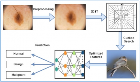
The proposed system architecture for diagnosing skin cancer, which utilizes image processing and DL approaches with dermoscopic images is discussed in this section. It is a pattern recognition system, organized into four important modules: These modules include preprocessing by median filters, image representation of dermoscopic images by 3DST, selection of directional sub-bands and features using CS algorithm, and classification by a simple ten-layer neural network. The proposed DLCS-3DST system is shown in Figure 1.
Figure 1. Proposed DLCS-3DST system
3.1 Preprocessing
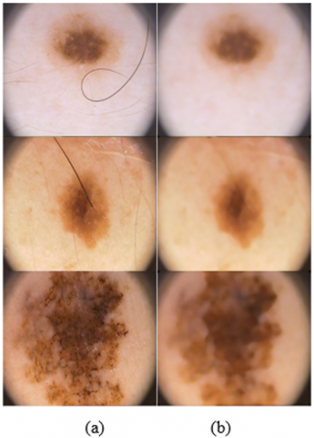
The initial step of this study employs a preprocessing stage to eliminate unwanted elements such as hairs and sounds from the dermoscopic images. This is achieved by utilizing a median filtering strategy. The purpose of this filter is to identify the middle value within a predetermined group of pixels and then replace the central pixel with that median value. It has the following benefits compared to mean filters: it preserves more gradient information and is less vulnerable to spurious noise within the neighbourhood. It preserves the edge information while eliminating noise without introducing any new colour values. The proposed system uses a 21×21 kernel for removing hair and noise effectively [7]. The original dermoscopic image and its median filtered images are shown in Figure 2.
Figure 2. (a) Input images (b) median filtered images
3.2 Representation of dermoscopic images
The primary objective of utilizing frequency transformation techniques to represent images is to provide a suitable representation of the image for subsequent image processing tasks. The Fourier and Wavelet transformations are widely used and can be used for one-dimensional signals and two-dimensional images. Since the images or signals are obtained and saved digitally, both transforms are also applied to the discrete domain. Several advanced systems have been developed to provide better approximations of images compared to wavelet, including Contourlet [21], Curvelet [22], and Shearlet [23]. These transforms offer more directional sub-bands than wavelets at a specific level of decomposition. Since the initial development of Curvelet was in the continuous domain, hence, its implementation in the discrete domain is very challenging. Only two directional components for each scale are generated by the directionlet transform [24].
Curvelet and Contourlet transforms accurately identify the boundary curves within a smooth region exclusively. Nevertheless, Shearlet can identify curves even in areas that lack smoothness [25]. Therefore, the Shearlet transform is employed as a strategy for extracting features. In this study, the NSST is employed due to its adherence to the translation-invariance property. The Shearlet is defined as:
$\psi_{a s t}(x)=\left|\operatorname{det} M_{a s}\right|^{-1 / 2} \psi\left(M_{a s}^{-1}(x-t)\right)$ (1)
where, the translation variable is represented by t, the shear variable is represented by s and the scale variable is represented by a. $M_{a s}$ is the product of dilation ($A_a$) and shear ($\left(B_s\right)$) which are represented by:
$A_a=\left[\begin{array}{cc}a & 0 \\ 0 & a^{\frac{1}{2}}\end{array}\right] where \ a>0$ (2)
$B_s=\left[\begin{array}{ll}1 & s \\ 0 & 1\end{array}\right]$ (3)
where, s is an integer.
A classical Shearlet ($\psi$) in the frequency domain is defined as:
$\hat{\psi}(\xi)=\hat{\psi}\left(\xi_1, \xi_2\right)=\hat{\psi}_1\left(\xi_1\right) \hat{\psi}_2\left(\frac{\xi_2}{\xi_1}\right)$ (4)
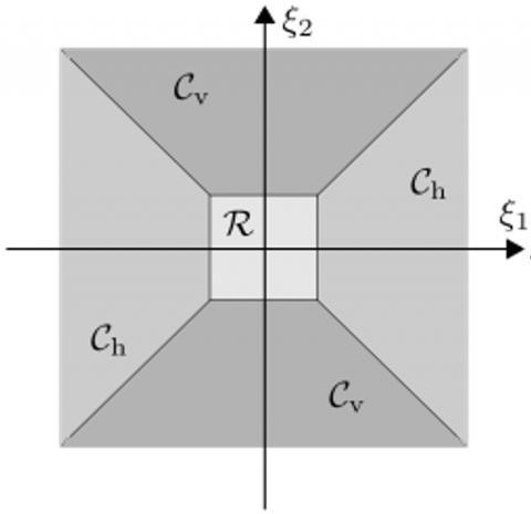
where, $\hat{\psi}_1$ and $\hat{\psi}_2$ be the wavelet function that belongs to subspaces of $L^2(\Re)$ and their corresponding Fourier transforms also belong to the space $C^{\infty}(\Re)$. The frequency domain of the Shearlet transform is shown in Figure 3 where the truncated cone regions are represented by $C_h$ and $C_v$ [25].
Figure 3. Frequency domain by discrete shearlet
The definitions for $C_h$ and $C_v$are:
$C_h=\left\{\left(\xi_1, \xi_2\right) \in \Re^2:\left|\frac{\xi_2}{\xi_1}\right| \leq 1,\left|\xi_1 \geq 1\right|\right\}$ (5)
$C_v=\left\{\left(\xi_1, \xi_2\right) \in \Re^2:\left|\frac{\xi_2}{\xi_1}\right|>1,\left|\xi_1 \geq 1\right|\right\}$ (6)
Based on the cone regions (d) in Eqs. (5) - (6), Eq. (1) can be rewritten as:
$L^2\left(\tilde{C}_d\right)=\left\{f \in L^2\left(\Re_2\right): \operatorname{supp} \hat{\mathrm{f}} \subset \tilde{\mathrm{C}}_{\mathrm{d}}\right\}$ (7)
3.3 Selection of directional sub-bands
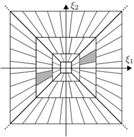
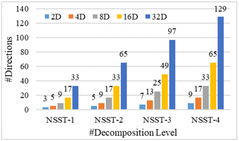
The initial step is representing the provided dermoscopic image using NSST at different decomposition levels. It generates many directional Sub-Bands (SB) with valuable information about the decomposed image. Figure 4 displays the NSST SBs corresponding to various levels and orientations.
Figure 4. Number of NSST sub-bands corresponding to various levels and orientations
Due to the large dimensionality of the NSST coefficient feature space, a statistical t-test is utilized. Based on the SBs’ energy levels in Eq. (8), a predominant SB of size XxY is chosen.
Energy $=\frac{1}{X Y} \sum_{i=1}^X \sum_{j=1}^Y\left|S B_{i j}\right|$ (8)
where, i, j are the co-ordinates of SB. Energy characteristics are extracted from specific levels and orientations of dermoscopic images belonging to two groups. To determine the SB that exhibits a significant difference between normal (A) and abnormal (B) with $n_A$ and $n_B$ samples, the t-test in Eq. (9) is used.
$\operatorname{tscore}(x)=\left(M_A(x)-M_B(x)\right) / \sqrt{\frac{S_A^2(x)}{n_A}+\frac{S_B^2(x)}{n_B}}$ (9)
where, Mx and Sx represent the mean and standard deviations of class x. Once the t-score has been calculated for all directional SBs at each level, the SB with the highest t-score is selected, indicating that it is significantly different from the others. The chosen directional SB is used to extract characteristics.
3.4 Selection of dominant features
After selecting the directional SB, the dominant Shearlet coefficients are selected using CS algorithm [26], a nature-inspired optimization algorithm. It mimics the brood parasitic conduct observed in certain cuckoo species, along with the Lévy flight behaviour exhibited by birds and fruit flies. For optimization, the following assumptions or rules are made:
• Each cuckoo lays a single egg and dumps it in a nest chosen at random.
• Nests that contain high-quality eggs (solutions) are passed on to the next generation.
• The quantity of accessible host nests remains constant, and a host bird has a likelihood ($p_a \in[0,1]$) of encountering an extraneous egg. Under these circumstances, the host bird will either discard the egg or abandon the nest and construct a new nest elsewhere.
An important component of CS is the utilization of Lévy flights to improve the overall ability to search globally. Lévy flights are a type of random walk where the distances between steps are determined by a probability distribution that has a strong tail. The step length (L) can be described by the Lévy distribution:
$L \sim \operatorname{Le} v y(\lambda) \propto|s|^{-\lambda},(1<\lambda \leq 3)$ (10)
The algorithm can be summarized as follows:
Initialization: A population of $n$ host nests $\left\{x_i\right\}$, where $i=$ $1,2, \ldots n$. Set algorithm parameters, including $p_a$ and $\lambda$.
Generate New Solutions: For each cuckoo $i$, generate a new solution $x_i^{t+1}$ using a Lévy flight: $x_i^{t+1}=x_i^t+\alpha \cdot L(s, \lambda)$ where $\alpha$ is the step size scaling factor, and $L(s, \lambda)$ represents the step length drawn from the Lévy distribution.
Evaluate Fitness: Evaluate the fitness of the new solution $f\left(x_i^{t+1}\right)$. If it is better than the current solution $f\left(x_j^t\right)$ in a randomly chosen nest $j$, replace $j$ with $i$.
Abandoning Poor Solutions: Abandon a fraction $p_a$ of the worse nests and build new ones at new locations using randomization: $x_j^{t+1}=x_j^t+\beta \cdot\left(x_i^t-x_k^t\right)$, where $x_i$ and $x_k$ re two randomly selected solutions, and $\beta$ is a random number drawn from a uniform distribution.
Selection of Best Solutions: Select the best solutions or nests based on their fitness values for the next iteration.
Iteration: Repeat steps 2-5 until the termination criterion is met, typically a maximum number of generations or a convergence threshold.
The use of Lévy flights ensures that the search process can escape local optima, enhancing global search capabilities. The algorithm is easy to implement and requires few parameters to tune. It can be applied to a wide range of optimization problems without significant modifications. In the proposed DLCS-3DST system, feature selection is performed using the CS algorithm, where the subset size is not predefined but adaptively determined during the optimization process. Each candidate solution (or "nest") in CS algorithm is encoded as a binary vector of length N where N is the total number of features extracted via the DST. A value of '1' at a given index indicates that the corresponding feature is selected, while '0' indicates exclusion. Thus, the number of selected features S in a solution corresponds to the number of ones in the binary vector. The objective function ($f(x)$) is defined by:
$f(x)=w \times C E+(1-w) \frac{S}{N}$ (11)
where, $f(x)$ is the fitness function, CE is the classification error rate, and w is a constant controlling the classification performance to the number of features used. The parameter values for the CS are selected based on a combination of empirical testing and literature guidelines. Specifically, the discovery probability ($P_a$) is set to 0.25 and the step size scaling factor ($\alpha$) to 1.5, consistent with values recommended in Yang and Deb [26]. These settings provided the best trade-off between convergence speed and classification performance to diagnose skin cancer. The proportion of selected features is defined by S/N in Eq. (11).
3.5 Classification
Neural networks are a computational approach that mimics the functioning of the human brain to analyze numerical data and then establish complex connections between input and output. Typically, these networks are trained using back-propagation techniques, which further improve the error function using gradient descent. They include non-linearity by incorporating a layer of hidden processing units.
The proposed DLCS-3DST system uses ten hidden layers for DL features. The connection between the input nodes and the hidden layer is trained using the chain rule to calculate the gradient of the error function for each weight. Widrow-Hoff learning rule is employed to update the weights between hidden layer and output layer. During training, cross-entropy loss is utilized in this study to update the weights and is shown in Eq. (12):
$Cross\ Entropy \ Loss =-\sum_{n=1}^m t_n \log \left(s_n\right)$ (12)
where, true label $t_n$ and the sigmoid function output $s_n$ and total number of classes (m). The activation function used in the hidden layer is given in Eq. (13), which is a Rectified Linear Unit (ReLU) function. It is defined for an input value (I) by:
$O=\max (0, I)$ (13)
where, O is the input value. It is observed from Eq. (13) that the function propagates just positive values while disregarding the negative values. The outcome of a particular layer is passed on to the next layer in a sequential manner. Ultimately, the predictions will be determined by the softmax layer, which utilizes the distribution of probabilities of the kth output layer. It is defined by:
$O\left(y_x\right)=\frac{e^{o_x}}{\sum_k e^{o_k}}$ (14)
where, xth layer’s output is denoted by ox. Table 1 provides the neural network parameters used in the DLCS-3DST system.
Table 1. DLCS-3DST system - network parameters
|
Parameters |
Settings |
|
Epochs/iterations |
200 |
|
hidden layers |
10 |
|
Optimizer |
Gradient Descent |
|
Learning rate |
0.01 |
|
Momentum |
0.9 |
|
Loss function |
Cross-entropy |
|
Dropout |
0.5 |
|
Activation function |
Rectified Linear (Hidden layer) & Softmax (Output layer) |
The simulation settings presented in Table 1 represent the optimal combination that yields the highest performance for the proposed DLCS-3DST system. These settings are selected by iterative experimentation.
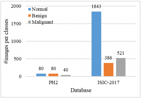
The PH2 database [27] is used to conduct an analysis of the designed DLCS-3DST system. More than two hundred dermoscopic colour images (RGB), including melanocytic lesions, are included in PH2. The dermoscopic images stored (200 images) in the database have a resolution of 768 by 560 pixels. Another powerful benchmark database, ISIC 2017 [28], is also used to do more analysis on the system. The ISIC 2017 database contains a total of 2750 images. Figure 5 shows the distribution of images in both databases.
Figure 5. Database distribution (image for each category)
To achieve optimal performance, it is necessary to have a larger quantity of images for training the DL architecture. Additionally, image augmentation is employed to address the issue of class imbalance by increasing the images in the dataset. The PH2 database images have been augmented from 200 to 3000 (1000 per category), while the ISIC images have been augmented from 2000 to 6000 (2000 per category) for analysis purposes. To achieve a balanced dataset for robust model training, a structured augmentation strategy is implemented, primarily using image rotation combined with other simple transformations.
For the PH2 dataset, each image in the normal and benign classes (originally 80 images each) was augmented 12 times using rotations at various angles (±15°, ±30°, ±45°), along with horizontal and vertical flips, scaling (Zoom in/out), and brightness adjustments, resulting in approximately 1000 images per class. The malignant class, with only 40 original images, required a more intensive augmentation scheme with 24 variants per image using a wider range of rotations (±10° to ±90°), flips, scaling, brightness/contrast changes, and Gaussian noise, to generate a total of 1000 images.
For the ISIC-2017 dataset, the normal class needed minimal augmentation, with just 157 additional samples created through light rotation and flipping. In contrast, the benign and malignant classes required 5 and 3 augmentations per image, respectively. These augmentations included combinations of rotations (±15° to ±60°), flips, scaling, and contrast adjustment to expand each class to 2000 images. This rotation-centered augmentation approach ensures class balance, enhances data diversity, and mitigates overfitting during model training. The DLCS-3DST system’s performance is assessed by empirically testing the system by counting the misclassifications on a testing set. It is important that the samples in both testing and training are statistically distinct. To evaluate the generalization performance of the proposed DLCS-3DST system, the dataset is split into training (60%), validation (20%), and test (20%) sets. The DLCS-3DST system is trained exclusively on the training set, with parameters such as the number of selected features and the controlling parameter (w) being tuned using the validation set. Final performance metrics are computed on the test set, which remained completely unseen during both training and validation. The consistent performance across validation and test sets indicates that the DLCS-3DST system generalizes well to unseen data. Table 2 shows the confusion matrix for a 3-class problem and the performance measures used for evaluating the proposed DLCS-3DST system.
To analyze the performance of the DLCS-3DST system, performance criteria such as sensitivity, specificity, and accuracy are computed from the obtained parameters TP, TN, FP, and FN. Table 3 shows the performances of the DLCS-3DST system on PH2 database images.
Table 2. Confusion matrix - 3-class problem and performance measurements
|
Confusion Matrix |
Parameters |
Performance Measures |
||||||
|
|
CL1 |
CL2 |
CL3 |
TP |
TN |
FP |
FN |
|
|
CL1 |
P11 |
P12 |
P13 |
P11 |
P22+ P23+P32+P33 |
P21+ P31 |
P12+ P13 |
Accuracy $=\frac{T P+T N}{T P+F N+T N+F P}$ |
|
CL2 |
P21 |
P22 |
P23 |
P22 |
P11 +P31+P13+P33 |
P12+ P32 |
P21+ P23 |
Sensitivity $=S_n=\frac{T P}{T P+F N}$ |
|
CL3 |
P31 |
P32 |
P33 |
P33 |
P11 + P12+P21+P22 |
P13+ P23 |
P31+ P32 |
Specificity $=S_p=\frac{T N}{T N+F P}$ |
|
where, CLj represents jth class, Pxy is the predicted class ‘y’ for the class ‘x’. |
||||||||
Table 3. Performances of the DLCS-3DST system on PH2 database images
|
Dir |
Lev |
Performance Measures |
||
|
Accuracy |
Sensitivity |
Specificity |
||
|
2D |
1 |
83.00 |
74.50 |
87.25 |
|
2 |
86.44 |
79.67 |
89.83 |
|
|
3 |
89.22 |
83.83 |
91.92 |
|
|
4 |
85.89 |
78.83 |
89.42 |
|
|
4D |
1 |
90.00 |
85.00 |
92.50 |
|
2 |
93.22 |
89.83 |
94.92 |
|
|
3 |
96.00 |
94.00 |
97.00 |
|
|
4 |
92.89 |
89.33 |
94.67 |
|
|
8D |
1 |
93.11 |
89.67 |
94.83 |
|
2 |
96.78 |
95.17 |
97.58 |
|
|
3 |
99.22 |
98.83 |
99.42 |
|
|
4 |
96.33 |
94.50 |
97.25 |
|
|
16D |
1 |
91.44 |
87.17 |
93.58 |
|
2 |
95.11 |
92.67 |
96.33 |
|
|
3 |
96.78 |
95.17 |
97.58 |
|
|
4 |
94.89 |
92.33 |
96.17 |
|
|
32D |
1 |
88.00 |
82.00 |
91.00 |
|
2 |
92.44 |
88.67 |
94.33 |
|
|
3 |
95.67 |
93.50 |
96.75 |
|
|
4 |
91.44 |
87.17 |
93.58 |
|
The selection of decomposition levels (#Lev) and directional components (#Dir) in the DST plays a critical role in capturing discriminative features for classification tasks. The proposed system empirically evaluated multiple configurations to determine the optimal parameters for skin lesion image analysis such as four decomposition levels and increasing numbers of directional sub-bands (2, 4, 8, 16, and 32) at each level. It is observed from Table 3 that the DLCS-3DST system’s performance for skin cancer classification reveals notable trends. Increasing the number of directions from 2D to 32D generally improves classification metrics. For instance, at the highest level (Level 3), the accuracy rises from 89.22% for 2D to 99.22% for 8D and then reduces to 96.78% for 16D. Sensitivity and specificity measures also show an upward trend with increasing directions and levels of DST. Notably, the system achieves a maximum sensitivity of 98.83% and specificity of 99.42% at Level 3 with 8D directions. Too few directions (2 and 4) at low-level (Level 1 and Level 2) may not capture the complex orientations of lesion textures, potentially degrading classifier performance. The third level with 8 directions provided the most effective balance, enabling the DST to capture rich, directional information while maintaining compactness and robustness in the feature set. While increasing the number of directions (16 and 32) theoretically enhances the angular resolution and ability to capture fine orientation-specific features. However, they can introduce noise and reduce the discriminative power of the extracted features. Additionally, it increases the dimensionality of the feature space, which may negatively affect classifier generalization. Thus, 8D at level 3 provided an optimal trade-off between richness of directional representation and feature compactness.
While analyzing the misclassified samples, it is observed that misclassifications predominantly occurred in cases characterized by low contrast, ambiguous pigmentation, or indistinct lesion borders. These features often lead to overlapping intra-class and inter-class feature representations in the latent space, thereby reducing classification confidence. This limitation underscores the potential benefit of incorporating auxiliary clinical metadata such as anatomical site, patient demographics, or lesion evolution history as additional input modalities. Such multimodal fusion could enhance the model's discriminative capacity in challenging scenarios and mitigate feature ambiguity arising from visually similar lesion types.
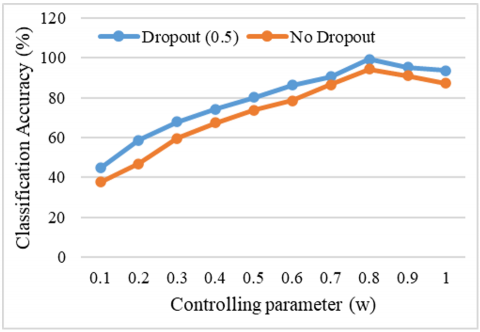
The effect of controlling parameter (w) in Eq. (10) for skin cancer classification is shown in Figure 6 by varying w from 0.1 to 1 with an increasing value of 0.1. The objective function in Eq. (11) encourages the CS algorithm to find a balance between minimizing classification error and reducing the number of features. As a result, the optimal subset size S emerges empirically during the search process. Experiments showed that CS algorithm typically selected around ~35% of the original feature set, demonstrating its effectiveness in producing compact and discriminative feature subsets without requiring manual specification of the subset size.
Figure 6. Performances of the proposed DLCS-3DST system for different values of w
The observations drawn from Figure 6 show intriguing patterns in the system's performance as it relates to different values of w. As "w" increases from 0.1, the system's performance gradually improves. This improvement is attributed to the incorporation of increasingly dominant features within the selected subset. This relationship between "w" and the performances of the proposed system highlights that the inclusion of dominant features enhances the model's predictive capabilities. Upon attaining the highest accuracy (w=0.8), the system's performance begins to decrease. This is due to the incorporation of redundant features into the subset. Moreover, it's notable that the system defaults to utilizing the entire set of features for performance evaluation when "w" reaches 1. Further analysis of the proposed systems is done on ISIC database images, and the performances are shown in Table 4.
Table 4. Performances of the DLCS-3DST system on ISIC database images
|
Dir |
Lev |
Performance Measures |
||
|
Accuracy |
Sensitivity |
Specificity |
||
|
2D |
1 |
83.44 |
75.17 |
87.58 |
|
2 |
86.83 |
80.25 |
90.13 |
|
|
3 |
89.50 |
84.25 |
92.13 |
|
|
4 |
86.27 |
79.40 |
89.70 |
|
|
4D |
1 |
90.22 |
85.33 |
92.67 |
|
2 |
93.33 |
90.00 |
95.00 |
|
|
3 |
96.22 |
94.33 |
97.17 |
|
|
4 |
93.28 |
89.92 |
94.96 |
|
|
8D |
1 |
93.39 |
90.08 |
95.04 |
|
2 |
97.06 |
95.58 |
97.79 |
|
|
3 |
99.39 |
99.08 |
99.54 |
|
|
4 |
96.67 |
95.00 |
97.50 |
|
|
16D |
1 |
91.78 |
87.67 |
93.83 |
|
2 |
95.22 |
92.83 |
96.42 |
|
|
3 |
97.11 |
95.67 |
97.83 |
|
|
4 |
94.96 |
92.44 |
96.22 |
|
|
32D |
1 |
88.17 |
82.25 |
91.13 |
|
2 |
92.83 |
89.25 |
94.63 |
|
|
3 |
96.06 |
94.08 |
97.04 |
|
|
4 |
91.72 |
87.58 |
93.79 |
|
It is observed from Table 4 that the same performance trend as PH2 is noticed for ISIC database images. The proposed DLCS-3DST system gives a maximum classification accuracy of 99.39% for ISIC images at 3L-8D features. The computational complexity of the proposed system is primarily influenced by the 3DST decomposition and the CS optimization. The average classification time per image is approximately 0.65 seconds on an Intel i7 processor with 16GB RAM and an NVIDIA GTX 1080 GPU, indicating feasibility for near-real-time clinical applications.
To validate the robustness of the results, a statistical significance analysis is performed over 10 independent runs using different training and testing samples. For both databases, the mean performance and 95% confidence intervals (CIs) are computed for accuracy, sensitivity and specificity. Table 5 shows the classification performance (mean ± 95% CI) of the DLCS-3DST system.
Table 5. Classification performance (mean ± 95% CI) of the DLCS-3DST system
|
Database |
Performance Measure (%)$\pm$95%CI |
||
|
Accuracy |
Sensitivity |
Specificity |
|
|
PH2 |
99$\pm$0.22 |
98.51$\pm$0.33 |
99.25$\pm$0.16 |
|
ISIC |
99.16$\pm$0.21 |
98.73$\pm$0.31 |
99.37$\pm$0.15 |
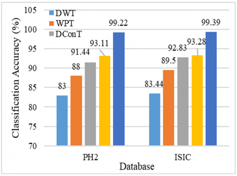
The results in Table 5 demonstrate high stability and consistent performance across multiple runs, as evidenced by the narrow 95% CI. This confirms that the system's performance is not due to randomness or chance, thus supporting the statistical robustness of the model. The skin cancer diagnosis performance in terms of classification accuracy of four different techniques, such as DWT [29], WPT [30], DConT [21], DCurT [22], and the proposed DLCS-3DST [23] system, is evaluated on the PH2 and ISIC skin lesion datasets. Figure 7 shows the performance comparison of state-of-the-art image representation systems.
Figure 7. Performance comparison of state-of-the-art image representation systems
It can be seen from Figure 7 that the DWT [29] achieved 83% on PH2 and 83.44% on ISIC database, and the WPT [30] improved upon DWT, attaining 88% (PH2) and 89.5% (ISIC). Both can capture both time and frequency information, making it well-suited for texture-based feature extraction. However, it lacks directional selectivity, which limits its performance in handling lesions with complex boundaries. DConT [21] achieved 91.44% on PH2 and 92.83% on ISIC as it captures smooth contours and edges compared to wavelet methods. The DCurT [22] slightly outperformed DConT, reaching 93.11% (PH2) and 93.28% (ISIC) due to that it can capture curve-like features and elongated structures, which are commonly found in medical images. Its high directional sensitivity and edge representation make it highly effective for boundary-aware skin lesion analysis. When compared to DWT, WPT, DConT and DCurT, 3DST can effectively capture complex lesion morphology and pigment distribution, resulting in a highly robust and generalizable feature representation. Hence, the proposed DLCS-3DST achieved the highest performance across both datasets, with 99.22% on PH2 and 99.39% on ISIC.
The multi-scale and multi-directionals models DConT and DCurT showed notable improvements, reaching accuracy of up to 93.28% on the ISIC dataset. However, the proposed 3DST method significantly outperformed all other approaches, achieving the highest classification accuracies of 99.22% on PH2 and 99.39% on ISIC. These results underscore the superior feature representation and generalization capability of the 3DST framework across diverse datasets, especially in comparison with traditional approaches.
An efficient DLCS-3DST system for dermoscopic image classification is presented in this paper. The undesired information such as noises and hairs that affects system performance is removed at first using median filtering. The proposed DLCS-3DST system selects texture descriptors using CS from the dominating SBs of 3DST, and then ten-layer DLCS uses these features to provide classification of dermoscopic images. Two databases; PH2 and ISIC 2017 are utilized for performance evaluation. Results demonstrate that the DLCS-3DST system achieves a classification accuracy of 99.22% using PH2 images and 99.39% using ISIC images when the features are extracted from 3rd levels and 8D. The most correlated SB at each level is chosen by statistical t-test. In future, the SB selection can be done out via optimization methods like in feature selection by CS. Though the evaluation of the proposed DLCS-3DST system is conducted on PH2 and ISIC datasets, the proposed DLCS-3DST system can be evaluated on external datasets such as HAM10000 and Dermofit. The robust performance on both PH2 and ISIC indicates promising generalization capabilities of the proposed DLCS-3DST system for skin cancer diagnosis.
[1] Jaisakthi, S.M., Mirunalini, P., Aravindan, C., Appavu, R. (2023). Classification of skin cancer from dermoscopic images using deep neural network architectures. Multimedia Tools and Applications, 82(10): 15763-15778. https://doi.org/10.1007/s11042-022-13847-3
[2] Naeem, A., Anees, T., Khalil, M., Zahra, K., Naqvi, R.A., Lee, S.W. (2024). SNC_Net: skin cancer detection by integrating handcrafted and deep learning-based features using dermoscopy images. Mathematics, 12(7): 1030. https://doi.org/10.3390/math12071030
[3] Shetty, B., Fernandes, R., Rodrigues, A.P., Chengoden, R., Bhattacharya, S., Lakshmanna, K. (2022). Skin lesion classification of dermoscopic images using machine learning and convolutional neural network. Scientific Reports, 12(1): 18134. https://doi.org/10.1038/s41598-022-22644-9
[4] Shen, X., Wei, L., Tang, S. (2022). Dermoscopic image classification method using an ensemble of fine-tuned convolutional neural networks. Sensors, 22(11): 4147. https://doi.org/10.3390/s22114147
[5] Thamizhamuthu, R., Maniraj, S.P. (2023). Deep Learning-Based Dermoscopic Image Classification System for Robust Skin Lesion Analysis. Traitement du Signal, 40(3): 1145-1152. https://doi.org/10.18280/ts.400330
[6] Midasala, V.D., Prabhakar, B., Chaitanya, J.K., Sirnivas, K., Eshwar, D., Kumar, P.M. (2024). MFEUsLNet: Skin cancer detection and classification using integrated AI with multilevel feature extraction-based unsupervised learning. Engineering Science and Technology, an International Journal, 51: 101632. https://doi.org/10.1016/j.jestch.2024.101632
[7] Maniraj, S.P., Sardarmaran, P. (2021). Classification of dermoscopic images using soft computing techniques. Neural Computing and Applications, 33(19): 13015-13026. https://doi.org/10.1007/s00521-021-05998-5
[8] Pitchiah, M.S., Rajamanickam, T. (2022). Efficient Feature Based Melanoma Skin Image Classification Using Machine Learning Approaches. Traitement du Signal, 39(5): 1633-1671. https://doi.org/10.18280/ts.390524
[9] Kumar, S.M., Kumanan, T. (2023). Skin Lesion Classification System Using Shearlets. Computer Systems Science & Engineering, 44(1): 833-844. https://doi.org/10.32604/csse.2023.022385
[10] Zareen, S.S., Sun, G., Kundi, M., Qadri, S.F., Qadri, S. (2024). Enhancing Skin Cancer Diagnosis with Deep Learning: A Hybrid CNN-RNN Approach. Computers, Materials & Continua, 79(1): 1497-1519. https://doi.org/10.32604/cmc.2024.047418
[11] Anupama, C.S.S., Yonbawi, S., Moses, G.J., Lydia, E.L., Kadry, S. (2023). Sand Cat Swarm Optimization with Deep Transfer Learning for Skin Cancer Classification. Computer Systems Science & Engineering, 47(2): 2079-2095. https://doi.org/10.32604/csse.2023.038322
[12] TR, G.B. (2020). An efficient skin cancer diagnostic system using Bendlet Transform and support vector machine. Anais da Academia Brasileira de Ciências, 92: e20190554. https://doi.org/10.1590/0001-3765202020190554
[13] Sudha, G., Birunda, M., Gnanasoundharam, J., Singh, J.A.J. (2023). Deep Learning System in Curvelet Domain for Skin Cancer Diagnosis. In 2023 4th International Conference on Electronics and Sustainable Communication Systems (ICESC), Coimbatore, India, pp. 1573-1577. https://doi.org/10.1109/ICESC57686.2023.10193507
[14] Wu, Q.E., Yu, Y., Zhang, X. (2023). A skin cancer classification method based on discrete wavelet down-sampling feature reconstruction. Electronics, 12(9): 2103. https://doi.org/10.3390/electronics12092103
[15] Lakshmi, V.V., Jasmine, J.L. (2021). A Hybrid Artificial Intelligence Model for Skin Cancer Diagnosis. Comput. Syst. Sci. Eng., 37(2): 233-245. http://dx.doi.org/10.32604/csse.2021.015700
[16] Fadaeian, A., Rahmani, A.E., Javid, R., Huang, Q., Alaoui, N., Adamou-Mitiche, A.B.H., Bouhamla, L. (2021). Classification of Melanoma Images Using Empirical Wavelet Transform. Journal homepage: http://iieta. org/journals/rces, 8(1): 1-8. https://doi.org/10.18280/rces.080101
[17] Jayaraman, P., Veeramani, N., Krishankumar, R., Ravichandran, K.S., Cavallaro, F., Rani, P., Mardani, A. (2022). Wavelet-based classification of enhanced melanoma skin lesions through deep neural architectures. Information, 13(12): 583. https://doi.org/10.3390/info13120583
[18] Tan, T.Y., Zhang, L., Lim, C.P. (2019). Intelligent skin cancer diagnosis using improved particle swarm optimization and deep learning models. Applied Soft Computing, 84: 105725. https://doi.org/10.1016/j.asoc.2019.105725
[19] Hosseinzadeh, M., Hussain, D., Zeki Mahmood, F.M., A. Alenizi, F., Varzeghani, A.N., Asghari, P., Lee, S.W. (2024). A model for skin cancer using combination of ensemble learning and deep learning. PloS One, 19(5): e0301275. https://doi.org/10.1371/journal.pone.0301275
[20] Claret, S.A., Dharmian, J.P., Manokar, A.M. (2024). Artificial intelligence-driven enhanced skin cancer diagnosis: leveraging convolutional neural networks with discrete wavelet transformation. Egyptian Journal of Medical Human Genetics, 25(1): 50. https://doi.org/10.1186/s43042-024-00522-5
[21] Do, M.N., Vetterli, M. (2005). The contourlet transform: an efficient directional multiresolution image representation. IEEE Transactions on image processing, 14(12): 2091-2106. https://doi.org/10.1109/TIP.2005.859376
[22] Candes, E.J., Donoho, D.L. (2005). Continuous curvelet transform: II. Discretization and frames. Applied and Computational Harmonic Analysis, 19(2): 198-222. https://doi.org/10.1016/j.acha.2005.02.004
[23] Lim, W.Q. (2010). The discrete shearlet transform: a new directional transform and compactly supported shearlet frames. IEEE Transactions on image processing, 19(5): 1166-1180. https://doi.org/10.1109/TIP.2010.2041410
[24] Velisavljevic, V., Beferull-Lozano, B., Vetterli, M., Dragotti, P.L. (2006). Directionlets: anisotropic multidirectional representation with separable filtering. IEEE Transactions on Image Processing, 15(7): 1916-1933. https://doi.org/10.1109/TIP.2006.877076
[25] Lessig, C., Petersen, P., Schäfer, M. (2019). Bendlets: A second-order shearlet transform with bent elements. Applied and Computational Harmonic Analysis, 46(2): 384-399. https://doi.org/10.1016/j.acha.2017.06.002
[26] Yang, X.S., Deb, S. (2009). Cuckoo search via Lévy flights. In 2009 World Congress on Nature & Biologically Inspired Computing (NaBIC), Coimbatore, India, pp. 210-214. https://doi.org/10.1109/NABIC.2009.5393690
[27] Mendonça, T., Ferreira, P.M., Marques, J.S., Marcal, A.R., Rozeira, J. (2013). PH 2-A dermoscopic image database for research and benchmarking. In 2013 35th Annual International Conference of the IEEE Engineering in Medicine and Biology Society (EMBC), Osaka, Japan, pp. 5437-5440. https://doi.org/10.1109/EMBC.2013.6610779
[28] Codella, N.C., Gutman, D., Celebi, M.E., Helba, B., Marchetti, M.A., Dusza, S.W., Halpern, A. (2018). Skin lesion analysis toward melanoma detection: A challenge at the 2017 international symposium on biomedical imaging (ISBI), hosted by the international skin imaging collaboration (ISIC). In 2018 IEEE 15th International Symposium on Biomedical Imaging (ISBI 2018), Washington, USA, pp. 168-172. https://doi.org/10.1109/ISBI.2018.8363547
[29] Mallat, S. (1999). A Wavelet Tour of Signal Processing. Elsevier. https://doi.org/10.1016/B978-0-12-374370-1.X0001-8
[30] Gao, R.X., Yan, R., Gao, R.X., Yan, R. (2011). Wavelet packet transform. Wavelets: Theory and Applications for Manufacturing, pp. 69-81. https://doi.org/10.1007/978-1-4419-1545-0_5