Abdenour Mekhmoukh*![]() | Salim Chelbi
| Salim Chelbi![]() | Reda Kasmi
| Reda Kasmi![]() | Riad Dib
| Riad Dib![]()
© 2025 The authors. This article is published by IIETA and is licensed under the CC BY 4.0 license (http://creativecommons.org/licenses/by/4.0/).
OPEN ACCESS
This paper presents a new algorithm for automatic skin cancerous ulcer detection, leveraging image processing and machine learning techniques to improve diagnostic accuracy. The proposed method consists of two main phases: learning and detection, preceded by a crucial pre-processing step to enhance image quality. The presence of hair can obscure ulcerated regions, leading to inaccurate detection. To address this, the DullRazor algorithm is applied, effectively removing hairs while preserving critical lesion details. This step ensures clearer feature extraction in subsequent stages. A dataset of 200 manually annotated ulcer images is analyzed to identify distinguishing characteristics. Three key reference feature vectors are derived: Texture (Capturing roughness and irregularity patterns), Relative Color (Comparing ulcer hues against surrounding healthy skin), and Color ( Identifying disease-specific pigmentations). An analysis window scans the lesion, comparing local features against the reference vectors. If the extracted features closely match, the region is classified as ulcerated. Distance metrics or machine learning classifiers likely determine similarity thresholds. Two methods are used to evaluate the suggested algorithm. A dermatologist will subjectively (qualitatively) determine if the detection is "Good", "Fairly good", or "not detected", objectively, based on whether the ulcer is there or not. The results of the proposed algorithm are encouraging, as they gave promising results.
carcinoma, Dullrazor algorithm, skin ulcer, dermoscopic images, features detection, image segmentation
The Basal cell carcinoma (BCC) is the most common of all cancers in North America and Europe [1], accounting for approximately 70% to 90% of carcinomas. It is common in men over the age of 50 [2]. In Switzerland, there are about 15,000 new cases of skin cancer [2]. This rate is much higher in the United States, where more than 3 million people are diagnosed with skin cancer each year [3].
In France, there are about 60,000 new cases (70 individuals per 100,000 inhabitants per year), and in Australia up to 400 cases per 100,000 inhabitants per year [4]. The surgical procedure is the most effective method to eliminate early cancerous lesions. Dermoscopy is effective in the naked eye diagnosis in terms of improving the detection rate of CBCs and reducing the number of biopsies [5, 6]. For wide screening, an automated system for the analysis of dermoscopy images is a practical, rapid, and objective tool for decision support.
The purpose of our work is to use image processing techniques to automate the detection of one of the characteristics of basal cell carcinoma, which is the ulcer. We will explain the different steps of the proposed algorithm, whose goal is the detection of ulcers in cancerous carcinoma lesions. After a pre-processing that consists of removing hair by the DullRazor method, the proposed algorithm consists of two phases. Learning and detection phase.
The implementation of the proposed algorithm is presented in Section 3. In Section 4 we present the performance of the proposed algorithm. Finally, the conclusion is presented in Section 5.
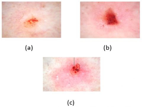
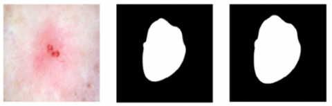
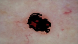
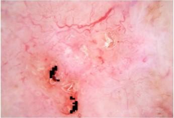
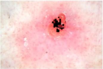
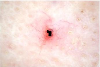
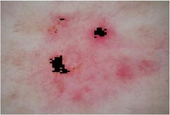
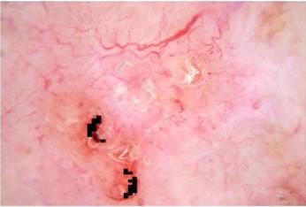
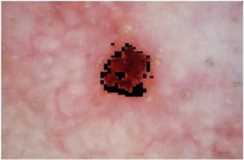
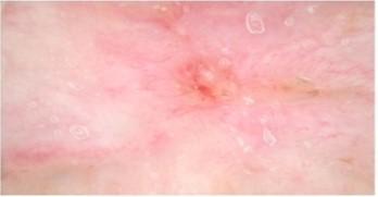
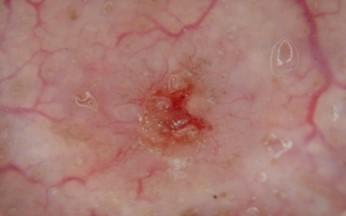
Ulcers are frequently seen in basal cell carcinoma lesions. An ulcer without a history of trauma, called "atraumatic", is an important identifier for basal cell carcinoma [7]. The ulcers change in intensity of the red color with time. The mild early ulcers appear bright red with a saturated color due to undiluted fresh blood (Figure 1 (a)), progress to larger areas (Figure 1 (b)), and finally appear reddish-brown and dry during the stage. healing (Figure 1 (c)) [7].
Figure 1. Ulcer evolution
2.1 Pre-processing
In order to remove the hairs that cover the lesion, the DullRazor algorithm [8] is used in Many techniques to remove hair and to cover lesion [9-11].
The algorithm is based on three basic steps:
A) Hair location
The three R, G, and B planes of the image are separately submitted to the closure morphological operation. Using the linear structuring element of 11 pixels according to the three orientations 0°, 45° and 90°.
$S_0=\left[\begin{array}{lllllllllllll}0 & 1 & 1 & 1 & 1 & 1 & 1 & 1 & 1 & 1 & 1 & 1 & 0\end{array}\right]$
$S_{90}=\left[\begin{array}{l}0 \\ 1 \\ 1 \\ 1 \\ 1 \\ 1 \\ 1 \\ 1 \\ 1 \\ 1 \\ 1 \\ 1 \\ 0\end{array}\right]$
$\mathrm{S}_{45}=\left[\begin{array}{lllllllll}0 & 0 & 0 & 0 & 0 & 0 & 0 & 0 & 0 \\ 0 & 1 & 0 & 0 & 0 & 0 & 0 & 0 & 0 \\ 0 & 0 & 1 & 0 & 0 & 0 & 0 & 0 & 0 \\ 0 & 0 & 0 & 1 & 0 & 0 & 0 & 0 & 0 \\ 0 & 0 & 0 & 0 & 1 & 0 & 0 & 0 & 0 \\ 0 & 0 & 0 & 0 & 0 & 1 & 0 & 0 & 0 \\ 0 & 0 & 0 & 0 & 0 & 0 & 1 & 0 & 0 \\ 0 & 0 & 0 & 0 & 0 & 0 & 0 & 1 & 0 \\ 0 & 0 & 0 & 0 & 0 & 0 & 0 & 0 & 0\end{array}\right]$
Tests have shown that these three structuring elements in the different orientations are more suitable for the detection of hairs. The DullRazor algorithm calculates for each closing operation, in the three directions, the maximum of matrix components obtained. The difference between the color component and the matrix obtained is calculated as:
$\mathrm{G}_{\mathrm{r}}=\left|\mathrm{I}_{\mathrm{r}}-\max \left(\mathrm{I}_{\mathrm{r}} \cdot \mathrm{S}_0, \mathrm{I}_{\mathrm{r}} \cdot \mathrm{S}_{90}, \mathrm{I}_{\mathrm{r}} \cdot \mathrm{S}_{45}\right)\right|$ (1)
$\mathrm{G}_{\mathrm{v}}=\left|\mathrm{I}_{\mathrm{v}}-\max \left(\mathrm{I}_{\mathrm{v}} \cdot \mathrm{S}_0, \mathrm{I}_{\mathrm{v}} \cdot \mathrm{S}_{90}, \mathrm{I}_{\mathrm{v}} \cdot \mathrm{S}_{45}\right)\right|$ (2)
$\mathrm{G}_{\mathrm{b}}=\left|\mathrm{I}_{\mathrm{b}}-\max \left(\mathrm{I}_{\mathrm{b}} \cdot \mathrm{S}_0, \mathrm{I}_{\mathrm{b}} \cdot \mathrm{S}_{90}, \mathrm{I}_{\mathrm{b}} \cdot \mathrm{S}_{45}\right)\right|$ (3)
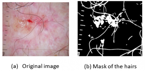
A binary mask M(x, y) is generated for each color component by comparing the value of each pixel with a predefined T empirical threshold (Figure 2).
$\mathrm{M}_{\mathrm{r}}(\mathrm{x}, \mathrm{y})=\left\{\begin{array}{c}1 \text { if } \mathrm{G}_r>\mathrm{T} \\ 0 \text { otherwise }\end{array}\right.$ (4)
Figure 2. Process results
The process is the same for the green and blue components. For maximum detection, the final mask of the hairs M of the original image is obtained by the union of the three masks red, green and blue.
$M=M_r \cup M_v \cup M_b$ (5)
B) Hair replacement
The mask M is used to locate the pixels of the bristles. The pixel is considered only if it is within a structure of maximum dimension greater than 50 and of minimum dimension of less than 10 pixels. For each pixel I (x, y) of the mask, the eight directions are considered. To avoid using pixel hair, the algorithm records the values I1 (x1, y1) and I2 (x2, y2) of the eleventh pixels from the edge of the hair, along the shortest line.
The new intensity value of the pixel I ( $\mathrm{x}, \mathrm{y}$ ) denoted $\mathrm{I}_{\mathrm{n}}(\mathrm{x}, \mathrm{y})$ depends on the pixels $\mathrm{I}_1$ and $\mathrm{I}_2$ as:
$\begin{aligned} & \mathrm{I}_{\mathrm{n}}(\mathrm{x}, \mathrm{y}) =\mathrm{I}_2\left(\mathrm{x}_2, \mathrm{y}_2\right) \frac{\mathrm{D}\left(\mathrm{I}(\mathrm{x}, \mathrm{y}), \mathrm{I}_1\left(\mathrm{x}_1, \mathrm{y}_1\right)\right)}{\mathrm{D}\left(\mathrm{I}_1\left(\mathrm{x}_1, \mathrm{y}_1\right), \mathrm{I}_2\left(\mathrm{x}_2, \mathrm{y}_2\right)\right)}+\mathrm{I}_1\left(x_1, y_1\right) \frac{\mathrm{D}\left(\mathrm{I}(\mathrm{x}, \mathrm{y}), \mathrm{I}_2\left(\mathrm{x}_2, \mathrm{y}_2\right)\right)}{\mathrm{D}\left(\mathrm{I}_1\left(\mathrm{x}_1, \mathrm{y}_1\right), \mathrm{I}_2\left(\mathrm{x}_2, \mathrm{y}_2\right)\right)}\end{aligned}$ (6)
where,
$\begin{aligned} D\left(I_2\left(x_2, y_2\right), I_1\left(x_1, y_1\right)\right)=\sqrt{\left(x_2-x_1\right)^2+\left(y_2-y_1\right)^2}\end{aligned}$ (7)
D: The Euclidean distance between the two pixels $I_2\left(x_2, y_2\right)$ and $I_1\left(x_1, y_1\right)$.
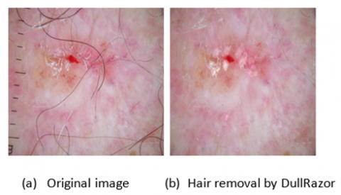
C) Smoothing
The algorithm proposes for this a smoothing by a window 5×5 follow of a morphological operation dilation with a structuring element square of size 5×5 [12, 13] (Figure 3).
Figure 3. DullRazor algorithm
2.2 Ulcer features extraction
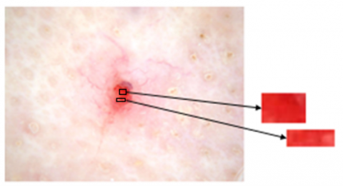
In order to identify the features that best represent the ulcer, features were extracted solely from the ulcer. To do this, parts of the ulcer are manually framed and saved as thumbnails image as shown in Figure 4. A base of 200 thumbnails is extracted and used to search for a reference vector.
Figure 4. Image extraction
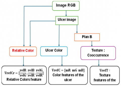
The extraction process of the reference characteristic vector is represented by the following flowchart (Figure 5).
Figure 5. Ulcer reference features extraction
2.3 Texture features
The texture features are extracted from the co-occurrence matrix for each blue (B) plane image. The choice of the plane and the parameters of the co-occurrence matrix: distance between a pair of pixels (d=1) and its orientation (θ=0) are fixed by experiment [14-16].
From each image, 23 Harlick features [17, 18] are calculated as follows:
$F 1=\sum_i \sum_j|i-j|^2 p(i, j)$ (8)
where,
p(i, j): standardized co-occurrence matrix.
$F 2=\sum \frac{p(i, j)}{1+|i-j|}$ (9)
Ng: number of distinct gray levels in the quantized image.
Is a measure of linear gray level dependencies in the image. Quantified with two equations.
$F 3=\sum_i \sum_j \frac{\left(i-\mu_x\right)\left(j-\mu_y\right) p(i, j)}{\sigma_x \sigma_y}$ (10)
where,
$\mu_x=\sum_i \sum_j i \cdot p(i, j)$
$\mu_y=\sum_{\mathrm{i}} \sum_{\mathrm{j}} \mathrm{j} \cdot \mathrm{p}(\mathrm{i}, \mathrm{j})$
$\sigma_{\mathrm{x}}=\sum_{\mathrm{i}} \sum_{\mathrm{j}}\left(\mathrm{i}-\mu_{\mathrm{x}}\right) \cdot \mathrm{p}(\mathrm{i}, \mathrm{j})$
$\sigma_y=\sum_i \sum_j\left(i-\mu_y\right) \cdot p(i, j)$
$F 4=\sum_i \sum_j \frac{(i, j) p(i, j)-\mu_x \mu_y}{\sigma_x \sigma_y}$ (11)
It measures the uniformity of the texture which is the repetition of the pairs of pixels.
$\mathrm{F} 5=\sum_{\mathrm{i}} \sum_{\mathrm{j}} \mathrm{P}(\mathrm{i}, \mathrm{j})^2$ (12)
This statistic is also called reversed moment of difference, it measures the homogeneity of the image; it is more sensitive to the presence of elements close to the diagonal in the GLCM and to a maximum value when all the elements of the image are identical.
$F 6=\sum_i \sum_j \frac{p(i, j)}{1+|i-j|}$ (13)
$F 7=\sum_i \sum_j \frac{p(i, j)}{1+|i-j| .^2}$ (14)
Measures the disorder of an image.
$\mathrm{F} 8=-\sum_{\mathrm{i}} \sum_{\mathrm{j}} \mathrm{p}(\mathrm{i}, \mathrm{j}) \cdot \log (p(i, j))$ (15)
$F 9=\sum_i \sum_j(i . j) p(i, j)$ (16)
$F 10=\sum_i \sum_j\left(i+j-\mu_x-\mu_y\right)^4 p(i, j)$ (17)
$F 11=\sum_i \sum_j\left(i+j-\mu_x-\mu_y\right)^3 p(i, j)$ (18)
$F 12=\sum_i \sum_j|i-j| p(i, j) \mid$ (19)
$\mathrm{F} 13=\max \mathrm{p}(\mathrm{i}, \mathrm{j})$ (20)
$F 14=\sum_i \sum_j(i-m)^2 p(i, j)$ (21)
where,
m: mean value of p (i, j).
$\mathrm{F} 15=\sum_{\mathrm{i}=2}^{2 \mathrm{~N}_{\mathrm{g}}} \mathrm{ip}_{\mathrm{x}+\mathrm{y}}(\mathrm{i})$ (22)
where, $\mathrm{p}_{\mathrm{x}+\mathrm{y}}(\mathrm{k})=\sum_{\mathrm{i}=1}^{\mathrm{N}_{\mathrm{g}}} \sum_{\mathrm{j}=1}^{\mathrm{N}_{\mathrm{g}}} \mathrm{p}(\mathrm{i}, \mathrm{j})$k=2, 3………, 2Ng.
$\mathrm{F} 16=-\sum_{\mathrm{i}=2}^{2 \mathrm{~N}_{\mathrm{g}}}\left(\mathrm{p}_{\mathrm{x}+\mathrm{y}}(\mathrm{i}) \cdot \log \left\{\mathrm{p}_{\mathrm{x}+\mathrm{y}}(\mathrm{i})\right\}\right)$ (23)
$\mathrm{F} 17=\sum_{\mathrm{i}=2}^{2 \mathrm{~N}_{\mathrm{g}}}(\mathrm{i}-\mathrm{F} 16)^2 \mathrm{p}_{\mathrm{x}+\mathrm{y}}(\mathrm{i})$ (24)
$\mathrm{F} 18=\sum_{\mathrm{i}=0}^{\mathrm{N}_{\mathrm{g}}-1} \mathrm{i}^2 \mathrm{p}_{\mathrm{x}-\mathrm{y}}(\mathrm{i})$ (25)
where, $\mathrm{p}_{\mathrm{x}-\mathrm{y}}(\mathrm{k})=\sum_{\mathrm{i}=1}^{\mathrm{N}_{\mathrm{g}}} \sum_{\mathrm{j}=1}^{\mathrm{N}_{\mathrm{g}}} \mathrm{p}(\mathrm{i}, \mathrm{j})$, k = 0, 1, .., Ng – 1.
$\mathrm{F} 19=-\sum_{\mathrm{i}=0}^{\mathrm{Ng}_{\mathrm{g}}-1} \mathrm{p}_{\mathrm{x}-\mathrm{y}}(\mathrm{i}) \log \left(\mathrm{p}_{\mathrm{x}-\mathrm{y}}(\mathrm{i})\right)$ (26)
$\mathrm{F} 20=\frac{\mathrm{HXY}-\mathrm{HXY} 1}{\max (\mathrm{HX}, \mathrm{HY})}$ (27)
where,
$\mathrm{HX}=-\sum_{\mathrm{i}} \mathrm{p}_{\mathrm{x}}(\mathrm{i}) \cdot \log \left(\mathrm{p}_{\mathrm{x}}(\mathrm{i})\right)$
$\mathrm{HY}=-\sum_{\mathrm{i}} \mathrm{p}_{\mathrm{y}}(\mathrm{i}) \cdot \log \left(\mathrm{p}_{\mathrm{y}}(\mathrm{i})\right)$
$H X Y=-\sum_i \sum_j p(i, j) \cdot \log (p(i, j))$
$H X Y 1=-\sum_i \sum_j p(i, j) \cdot \log \left(p_x(i) p_y(j)\right)$
$\mathrm{F} 21=(1-\exp \{-2(\mathrm{HXY} 2-\mathrm{HXY})\})^{1 / 2}$ (28)
where,
$H X Y 2=-\sum_i \sum_j p_x(i) p_y(j) \cdot \log \left\{p_x(i) p_y(j)\right\}$
$F 22=\sum_i \sum_j \frac{p(i, j)}{1+|i-j|^2 / N_g}$ (29)
$F 23=\sum_i \sum_j \frac{p(i, j)}{1+(i-j)^2 / N_g}$ (30)
Each image is defined by its feature vector.
$\left[\begin{array}{c}\text { Image 1 } \\ \text { Image 2 } \\ \text { Image 3 } \\ \cdot \\ \cdot \\ \cdot \\ \text { Image 200 }\end{array}\right]=\left[\begin{array}{cccc}F_{(1,1)} F_{(1,2)} F_{(1,3)} F_{(1,4)} & \ldots & F_{(1,22)} F_{(1,23)} \\ F_{(2,1)} F_{(2,2)} F_{(2,3)} F_{(2,4)} & \ldots & F_{(2,22)} F_{(2,23)} \\ F_{(3,1)} F_{(3,2)} F_{(3,3)} F_{(3,4)} & \ldots & F_{(3,22)} F_{(3,23)} \\ & \cdot & & \\ & \cdot & & \\ & \cdot & & \\ F_{(200,1)} F_{(200,2)} F_{(200,3)} F_{(200,4)} & \ldots & F_{(200,22)} F_{(200,23)}\end{array}\right]$
Subsequently, the texture reference vector (VrefT), which represents the ulcer features, is calculated as the median of the characteristic vectors of the 200 images,
$\begin{gathered}\text { VrefT }=[\operatorname{median}(F(i, 1)), \operatorname{median}(F(i, 2)), \ldots, \operatorname{median}(F(i, 23))]\end{gathered}$ (31)
2.4 Ulcer color features [18, 19]
The extracted color features are the medians of the R, G and B planes of the 200 ulcer images (Figure 6).
Figure 6. Ulcer images were decomposed into their respective red (R), green (G), and blue (B) planes
Each image is defined by its vector of color characteristics, which are the medians of the red (mR), green (mG), and blue (mB) planes.
$\left[\begin{array}{c}\text { Image 1 } \\ \text { Image 2 } \\ \text { Image 3 } \\ \cdot \\ \cdot \\ \cdot \\ \text { Image 200 }\end{array}\right]=\left[\begin{array}{ccc}m R 1 & m G 1 & m B 1 \\ m R 2 & m G 2 & m B 2 \\ m R 3 & m G 3 & m B 3 \\ & \cdot & \\ & \cdot & \\ m R 200 & m G 200 & m B 200\end{array}\right]$
The color reference vector VrefC is the median of the feature vectors of the 200 images.
VrefC $=\left[\begin{array}{c}\operatorname{median}(\mathrm{mR}(\mathrm{k})) \operatorname{median}(\mathrm{mG}(\mathrm{k})) \\ \operatorname{median}(\mathrm{mB}(\mathrm{k}))\end{array}\right]$ (32)
2.5 Relative colors
Relative color features use the colors of healthy skin and the color of the ulcer [20, 21]. Are calculated as:
(1) The mask is dilated using the morphological operator dilation with a disk structuring element of radius r=20. (Figure 7)
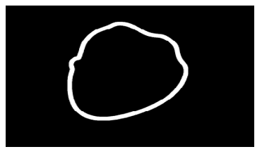
(2) The mask of the healthy skin surrounding the lesion is obtained from the subtraction between the dilated mask and the original image mask (Figure 8).
Using the mask of the skin (Figure 8), the measures MpeauR , MpeauG and MpeauB, which represent, respectively, the median of the red, green and blue planes of the skin are calculated.
(a) Original image (b) Lesion manual mask
Figure 7. Dilated mask
Figure 8. A mask of healthy skin surrounds the lesion
Relative colors are defined as:
relR $=$ MpeauR - MulcR (33)
The MulcR, MulcG and MMulcB represent, respectively, the median of the red, green and blue ulcer plane.
where, relR is the relative color of the ulcer area of the red plane. Similarly, relG and relB for the green and blue planes, respectively. Then, the vector of the relative ratios of color, which one notes VrefCr, is calculated like:
$V r e f C r=\left[\frac{r e l R}{r e l G}, \frac{r e l B}{r e l R}, \frac{r e l G}{r e l R}\right]$ (34)
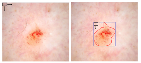
The idea is to scan the lesion by a dimension analysis window (10×15), the size of the window is chosen so that you can select the parts of the ulcer.
In order to reduce the sweeping time, the frame delimited by the ends of the contour of the lesion (manual contour) is scanned. Figure 9 shows how much space you can not sweep.
a) Without frame b) With frame
Figure 9. Gain of sweeping space
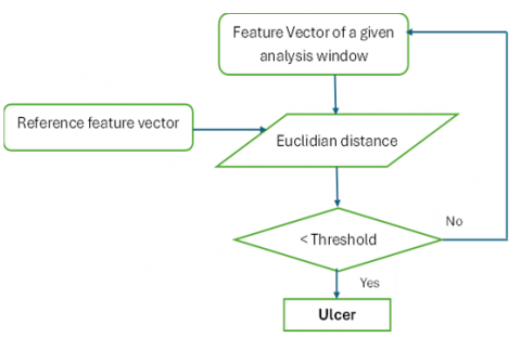
Figure 10. Principle of ulcer detection
From each analysis window, the three feature vectors (texture, color, and relative color) are measured. Then, we measure the difference of these three vectors with the reference feature vectors (texture: VrefT, color: VrefC, and relative color: VrefCr). By setting three empirical thresholds, a window is said to be ulcerated (selects an ulcer portion) if the difference is small enough. The following flowchart shows the principle of ulcer detection (Figure 10).
This section is devoted to the experimental part which consists of two steps. The first step is to set the different empirical thresholds used in the algorithm. The second step is to perform the proposed method on dermoscopic images of ulcerated CBC lesions to evaluate the performance of the proposed algorithm.
4.1 Datasets
A dataset of 50 dromoscopic images is used, early basal cell carcinoma (BCC) cancer, size 1024×768. All lesions have a non-traumatic ulcer. Some pictures are covered with hair. 20 images were used for learning, which consists in selecting the most discriminating characteristics (texture, color, and relative color) among the 29 extracts.
The skin ulcer exhibits greater chromatic variability (pigmentary heterogeneity), according to the clinical interpretation and experimentation which provides an objective threshold based on the actual data distribution, statistically validated, and clinically relevant for the detection of skin ulcer with High sensitivity (early detection) and High specificity (reduction of false positives)
Finally, the thresholds used for the three feature vectors, texture, color and relative color are fixed respectively as:
$\left\{\begin{array}{c}\text { Threshold } 1=25 \\ \text { Threshold } 2=0.455 \\ \text { Threshold } 3=0.45\end{array}\right.$
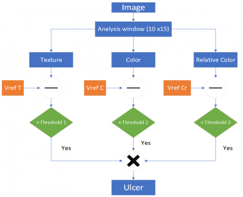
The following flowchart summarizes the process of ulcer detection in the analysis window (Figure 11).
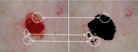
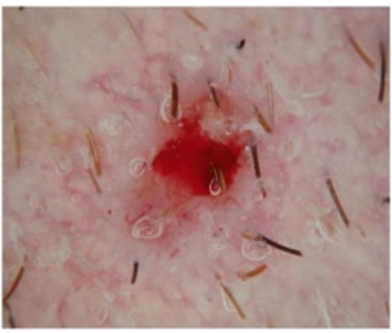
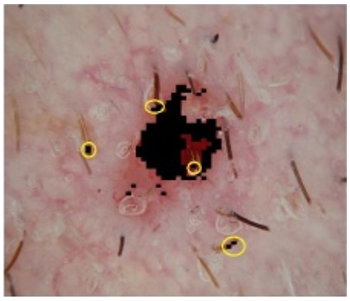
The use of the texture (23), color (3), and relative color (3) features, in addition to the ulcer, detects false positives, which are either veins or part of the reddish skin. Figure 12 shows the detection of circled false positives.
Since the principle of detection is to label an analysis window as an ulcer if its characteristics are similar or close to the reference characteristics (Vreft, VrefC, and VrefCr ). The comparison between the latter and the characteristics of the false positives allowed us to keep only 10 texture features, 3 color, and 1 relative color. Table 1 shows the selected features.
Figure 11. Ulcer detection
Table 1. Selected features
|
Features |
Equation |
Description |
|
Texture |
$\mathrm{F} 5=\sum_{\mathrm{i}} \sum_{\mathrm{j}} \mathrm{P}(\mathrm{i}, \mathrm{j})^2$ |
Energy |
|
$F 8=-\sum_i \sum_j p(i, j) \cdot \log (p(i, j))$ |
Entropy |
|
|
$F 9=\sum_i \sum_j(i . j) p(i, j)$ |
Auto-correlation |
|
|
$F 10=\sum_i \sum_j\left(i+j-\mu_x-\mu_y\right)^4 p(i, j)$ |
Cluster prominence |
|
|
$F 11=\sum_i \sum_j\left(i+j-\mu_x-\mu_y\right)^3 p(i, j)$ |
Cluster shadow |
|
|
$F 12=\sum_i \sum_j|i-j| p(i, j)$ |
Dissimilarity |
|
|
$F 14=\sum_i \sum_j(i-m)^2 p(i, j)$ |
Variance |
|
|
$\mathrm{F} 15=\sum_{\mathrm{i}=2}^{2 \mathrm{~N}_{\mathrm{g}}} \mathrm{i} \cdot \mathrm{p}_{\mathrm{x}+\mathrm{y}}$ (i) |
Mean sum |
|
|
$\mathrm{F} 16=-\sum_{\mathrm{i}=2}^{2 \mathrm{~N}_{\mathrm{g}}}\left(p_{x+y}(\mathrm{i}) \cdot \log \left\{p_{x+y}(\mathrm{i})\right\}\right)$ |
Entropy sum |
|
|
$\mathrm{F} 17=\sum_{\mathrm{i}=2}^{2 \mathrm{Ng}_{\mathrm{g}}}(\mathrm{i}-\mathrm{F} 16)^2 \mathrm{p}_{\mathrm{x}+\mathrm{y}}(\mathrm{i})$ |
Variance sum |
|
|
Color |
$m R$ $m G$ $m B$ |
Median of red plane Median of green plane Median of blue plane |
|
Relative Color |
$\frac{\text { relR }}{\text { relG }}$ |
Relative color of the ulcer area of the plane (R, G) |
(a) Original image (b) detection of false positives
Figure 12. Detection of false positives
|
a) with 29 features |
b) with 14 features |
Figure 13. Detection result
With :
Vref $T=\left[\begin{array}{llllllllll}3.300 & 1.104 & 0.169 & 0.043 & 0.753 & 0.491 & 3.261 & 3.429 & 10.314 & 0.463\end{array}\right]$
VrefC $=\left[\begin{array}{lll}0.69298 & 0.00030101 & 7.3407 \mathrm{e}-005\end{array}\right]$
VrefCr $=0.45$
Figure 13 shows the refinement of ulcer detection after removal of features that do not represent an ulcer (reduction from 29 to 14 characteristics).
To evaluate our algorithm, 60 images were used (30 healthy, 30 ulcers). The algorithm was evaluated in two ways: subjective evaluation by a dermatologist, and objective evaluation for each part of the classes.
4.2. Performance for metrics classifiers
In medical expression, instances are considered as positive, indicating the existence of the disease, and negative, indicating the absence of the disease; thus, four possibilities arise when medical images are submitted to the classifiers:
The metrics that were considered to evaluate the classifiers for these were:
accuaracy $=\frac{T P+T N}{T P+T N+F P+F N}$
precision $=\frac{T P}{T P+F P}$
recall $=\frac{T P}{T P+F N}$
With the help of dermatologist Dr ARROUDJ Aissa, quoted SOMACOB, Bejaia, we were able to evaluate our results by dividing them into three categories: "Good", "Pretty good ", and "Evil".
Ulcer tissue:
Healthy tissue:
4.3 Analyzing the result
This evaluation method is subjective, which is not optimal because of the lack of numerical measurements. Several works of segmentation of the dermoscopic lesions evaluated their results subjectively (well, rather well, badly ...), on the one hand because the manual segmentation differs from one dermatologist to another and on the other hand by lack of reference data.
The following Table 2 illustrates the subjective results obtained:
Table 2. Classification results
|
Detection |
Well and Pretty Detected |
Badly Detected |
Time Execution (mn) |
|
30 images (ulcer) |
28 |
2 |
24.825 |
|
29 |
1 |
20.317 |
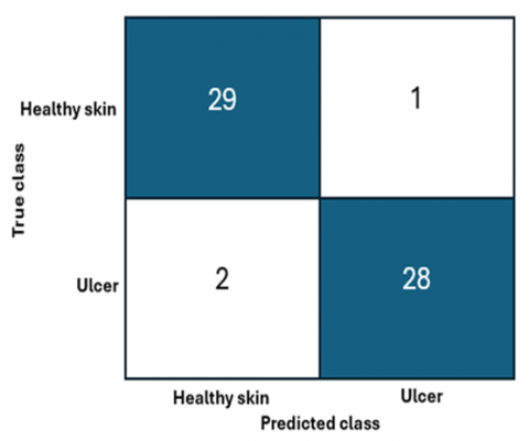
The confusion matrix of the method that describes the complete performance of the model is shown in Figure 14, this generates a accuracy of à.95 and precision of 0.96.
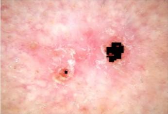
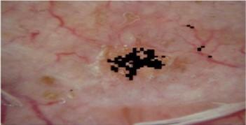
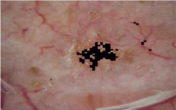
Figure 15 shows lesions with ulcer detection classified as "good and pretty good".
Figure 14. Confusion matrix
Figure 15. Ulcer good and pretty well detected
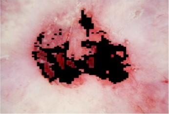
Figure 16. Ulcer badly detected
Figure 17. Ulcer not detected
Figure 18. Ulcer badly detected in the presence of bubbles due to immersion fluid
Figure 16 shows lesions with healthy skin classified as ulcer tissue.
Objectively the result of the algorithm is a binary classification, ulcer detected or not detected. In this case, 28 out of 30 lesions are classified as ulcerated during 24.825minut.
However, the healthy images are classified as healthy with a percentage of 96.6% during 20.317 minut.
Chino et al. [22] used the manually segmented ulcer characteristics in order to classify benign lesions and cancerous lesions of basal cell carcinoma type. This work has shown the feasibility of the goal. Extracted features are based on texture and color.
In this work, the features extracted by Serkan and al. Have been enhanced for the purpose of automating ulcer detection. Subjective evaluation, in first part on the total of 30 ulcerated lesions, the algorithm detected the ulcer in 28 images, and not detected in 2 images. In the last part, the 30 healthy images are classified as 29 healthy image as true negative and detect a false ulcer in the last image.
The objective evaluation showed a very good ability to identify the ulcer by the algorithm, 28 lesions well classified as ulcerated, or 93.33%. Figure 17, and Figure 18 illustrate the not detected ulcer.
(a) Original image
(b) Hairs as false positives
(c) After hair filtering
Figure 19. Results before and after hair removal
DullRazor has shown its effectiveness in hair removal and thus minimizes detection of false positives by our algorithm, see the Figure 19. Knowing that DullRazor filters black hair, it has been found that it can filter small areas of ulcer that appear black at the gray level.
In this paper, we have presented a new algorithm for skin cancerous ulcer detection. The first step is a pretreatment, which consists of removing the hairs covering the lesion and the ulcerated parts using the DullRazor algorithm. A set of 200 ulcer images are extracted manually, in order to study its characteristics. Three reference feature vectors based on texture, color and relative color, are selected.
The proposed algorithm is evaluated in two ways. Subjectively (qualitatively), by a dermatologist depending on whether the detection is "Good", "Fairly good" and "not detected". Objectively, according to the presence or absence of the ulcer. The two results showed that the algorithm is satisfactory. The results obtained are quite interesting, in a subjective way. In the first part the 30 ulcerated images, 28 were detected well and pretty well, and 2 were not detected, and objectively, 28 were detected and 2 not detected. In the second part; the 30 healthy images, 29 were classified as healthy images, and in the last images, an ulcer was detected, achieving at the end an accuracy of 95%.
Several improvements can be made to this algorithm by acting at the level of the filtering, in particular the filtering of bubbles due to the immersion liquid and the removal of hairs in an efficient manner without being able to touch the ulcer. A large image database will refine the choice of empirical thresholds, which is one of the important parameters that improve detection quality.
[1] Mohan, S.V., Chang, A.L.S. (2014). Advanced basal cell carcinoma: Epidemiology and therapeutic innovations. Current Dermatology Reports, 3(1): 40-45. https://doi.org/10.1007/s13671-014-0069-y
[2] Lear, W., Dahlke, E., Murray, C.A. (2007). Basal cell carcinoma: Review of epidemiology, pathogenesis, and associated risk factors. Journal of Cutaneous Medicine and Surgery, 11(1): 19-30. https://doi.org/10.2310/7750.2007.00011
[3] Rogers, H.W., Weinstock, M.A., Feldman, S.R., Coldiron, B.M. (2015). Incidence estimate of nonmelanoma skin cancer (keratinocyte carcinomas) in the US population, 2012. JAMA Dermatology, 151(10): 1081-1086. https://doi.org/10.1001/jamadermatol.2015.1187
[4] Roewert-Huber, J., Lange-Asschenfeldt, B., Stockfleth, E., Kerl, H. (2007). Epidemiology and aetiology of basal cell carcinoma. British Journal of Dermatology, 157(s2): 47-51. https://doi.org/10.1111/j.1365-2133.2007.08273.x
[5] Ackerman, A.B., Mones, J.M. (2006). Solar (actinic) keratosis is squamous cell carcinoma. British Journal of Dermatology, 155(1): 9-22. https://doi.org/10.1111/j.1365-2133.2005.07121.x
[6] Tüzün, Y., Kutlubay, Z., Engin, B., Serdaroğlu, S. (2011). Basal cell carcinoma. Skin Cancer Overview, Intech Open Access Publisher. http://doi.org/10.5772/25775
[7] Kefel, S., Guvenc, P., LeAnder, R., Stricklin, S.M., Stoecker, W.V. (2012). Discrimination of basal cell carcinoma from benign lesions based on extraction of ulcer features in polarized-light dermoscopy images. Skin Research and Technology, 18(4): 471-475. https://doi.org/10.1111/j.1600-0846.2011.00595.x
[8] Lee, T., Ng, V., Gallagher, R., Coldman, A., McLean, D. (1997). Dullrazor®: A software approach to hair removal from images. Computers in Biology and Medicine, 27(6): 533-543. https://doi.org/10.1016/S0010-4825(97)00020-6
[9] Fan, H., Xie, F., Li, Y., Jiang, Z., Liu, J. (2017). Automatic segmentation of dermoscopy images using saliency combined with OTSU threshold. Computers in Biology and Medicine, 85: 75-85. https://doi.org/10.1016/j.compbiomed.2017.03.025
[10] Garnavi, R., Aldeen, M., Celebi, M.E., Bhuiyan, A., Dolianitis, C., Varigos, G. (2010). Automatic segmentation of dermoscopy images using histogram thresholding on optimal color channels. International Journal of Medicine and Medical Sciences, 1(2): 126-134.
[11] Schmid-Saugeona, P., Guillodb, J., Thirana, J.P. (2003). Towards a computer-aided diagnosis system for pigmented skin lesions. Computerized Medical Imaging and Graphics, 27(1): 65-78. https://doi.org/10.1016/S0895-6111(02)00048-4
[12] Maragos, P., Pessoa, L.F. (1999). Morphological filtering for image enhancement and detection. The Image and Video Processing Handbook, 135-156. http://cvsp.cs.ece.ntua.gr/publications/jpubl+bchap/MaragosPessoa_MorphFilterEnhancDetect_ImVidHbk2000.pdf.
[13] Gonzalez, R.C. (2009). Fundamentals of Medical Imaging. Cambridge University Press. https://doi.org/10.1017/cbo9780511596803.002
[14] Soh, L.K., Tsatsoulis, C. (2002). Texture analysis of SAR sea ice imagery using gray level co-occurrence matrices. IEEE Transactions on Geoscience and Remote Sensing, 37(2): 780-795. https://doi.org/10.1109/36.752194
[15] Gómez, W., Pereira, W.C.A., Infantosi, A.F.C. (2012). Analysis of co-occurrence texture statistics as a function of gray-level quantization for classifying breast ultrasound. IEEE Transactions on Medical Imaging, 31(10): 1889-1899. https://doi.org/10.1109/TMI.2012.2206398
[16] Pereira, S.M., Frade, M.A.C., Rangayyan, R.M., de Azevedo Marques, P.M. (2011). Classification of dermatological ulcers based on tissue composition and color texture features. In Proceedings of the 4th International Symposium on Applied Sciences in Biomedical and Communication Technologies, New York, United States, pp. 1-6. https://doi.org/10.1145/2093698.2093766
[17] Haralick, R.M., Shanmugam, K., Dinstein, I.H. (1973). Textural features for image classification. IEEE Transactions on Systems, Man, and Cybernetics, 6: 610-621. https://doi.org/10.1109/TSMC.1973.4309314
[18] Clausi, D.A. (2002). An analysis of co-occurrence texture statistics as a function of grey level quantization. Canadian Journal of Remote Sensing, 28(1): 45-62. https://doi.org/10.5589/m02-004
[19] Pereira, S.M., Frade, M.A., Rangayyan, R.M., Azevedo-Marques, P. M. (2012). Classification of color images of dermatological ulcers. IEEE Journal of Biomedical and Health Informatics, 17(1): 136-142. https://doi.org/10.1109/titb.2012.2227493
[20] Azevedo-Marques, P.M., Pereira, S.M., Frade, M.A., Rangayyan, R.M. (2013). Segmentation of dermatological ulcers using clustering of color components. In 2013 26th IEEE Canadian Conference on Electrical and Computer Engineering (CCECE), Regina, Canada, pp. 1-4. https://doi.org/10.1109/CCECE.2013.6567776
[21] Dalila, F., Zohra, A., Reda, K., Hocine, C. (2017). Segmentation and classification of melanoma and benign skin lesions. Optik, 140: 749-761. https://doi.org/10.1016/j.ijleo.2017.04.084
[22] Chino, D.Y., Scabora, L.C., Cazzolato, M.T., Jorge, A.E., Traina-Jr, C., Traina, A.J. (2020). Segmenting skin ulcers and measuring the wound area using deep convolutional networks. Computer Methods and Programs in Biomedicine, 191: 105376. https://doi.org/10.1016/j.cmpb.2020.105376