Shankar Ganesan*![]() | Kalaiselvi Geetha Manoharan
| Kalaiselvi Geetha Manoharan![]() | Ezhumalai Periyathamb
| Ezhumalai Periyathamb![]()
© 2025 The authors. This article is published by IIETA and is licensed under the CC BY 4.0 license (http://creativecommons.org/licenses/by/4.0/).
OPEN ACCESS
Fog significantly reduces video clarity by lowering contrast, blurring objects, and distorting colors hampers scene understanding in critical applications such as autonomous driving, traffic surveillance, and remote sensing. Existing defogging methods like Retinex-based algorithms and dark channel prior often fail under varying fog densities and lack real-time adaptability, leading to detail loss or visual artifacts. To address these challenges, this study introduces a hybrid deep learning approach that integrates a Convolutional Neural Network (CNN) for fog level detection and a Generative Adversarial Network (GAN) for adaptive video defogging. The CNN accurately estimates fog density per frame, enabling the GAN to adjust its processing and preserve essential visual features. Preprocessing steps such as grayscale conversion and histogram equalization, enhance feature extraction and improve defogging performance. The system is designed for real-time deployment and adaptability across different atmospheric conditions. Evaluation using metrics such as PSNR, SSIM, FADE, NIQE, MAE, and RMSE demonstrates superior performance compared to existing and state-of-the-art methods like MSBDN and FFA-Net. Notably, under heavy fog, the proposed model achieved a PSNR of 26.0 dB, SSIM of 0.86, FADE score of 0.41, and runtime of 0.31 s/frame, confirming its efficiency and suitability for safety-critical, low-visibility environments.
fog detection, video defogging, deep learning, video enhancement, real-time processing, autonomous vehicles, environmental adaptability, video restoration
Monitoring fog plays a crucial role in meteorology for assessing climate and atmospheric conditions. Fog forecasting benefits various aspects of daily life, including environmental surveillance, agricultural productivity, and aviation safety. Fog can be categorized into five classes based on density: gentle fog, substantial fog, heavy fog, thick mist, and extremely dense fog [1]. Early methods of fog observation relied on the naked eye with observers gauging fog intensity by identifying objects at specific distances. Today, devices such as transmissometers and scatterometers automate the measurement of horizontal visibility. When local optical conditions differ from the broader atmosphere, autonomous systems may provide inaccurate readings. Large-scale deployment of these devices are costly and satellite-based fog monitoring is often unreliable due to cloud interference [2].
The rise of Artificial Intelligence (AI) and video recognition technologies has advanced fog transparency monitoring especially with the proliferation of security cameras across industries. For instance, introduced visibility estimation technique using B-spline wavelet transformations, while extracted road and sky areas to determine fog perception range [3]. Employed camera parameters and Region of Interest (ROI) extraction for visibility estimation, and utilized methods like linear regression, decision trees, edge detection, and contrast reduction between videos to estimate visibility [4]. Fog video analysis have relied on video feature-based techniques, which, despite their success, face limitations in adaptability and applicability. Developed a model using dark channels, local comparisons, and saturation parameters, training a random forest to predict visibility in various weather conditions [5]. Applied transfer learning improves prediction accuracy without requiring extensive training data. Proposed a method combining feature fusion and transfer learning for meteorological vision estimation, increasing reliability by integrating multiple data sources [6]. Used Particle Swarm Optimization (PSO) in a transferable learning approach for estimating transparency and FGS-Net built on empirical characteristic streams, proved effective in frequently foggy areas. Developed an automated technique using CCTV footage to detect marine fog and estimate visibility distance demonstrating the effectiveness of AI-driven approaches. These advancements highlight how AI and machine learning methods are reshaping fog monitoring, enhancing reliability and adaptability in varied environmental conditions [7].
Utilized a deep learning approach to improve visibility estimation in traffic videos, revealing that deep quantification methods enhanced brightness prediction accuracy. These methods often require large, well-balanced datasets for optimal performance. Deep learning models such as VGG16 and ResNet50 are effective for visibility estimation on extensive datasets though their accuracy drops significantly with limited data [8]. VGG16/19 relies on max-pooling and convolutional layers for feature extraction, but these layers increase processing costs. ResNet50 incorporates residual components to address vanishing gradient issues enabling deeper networks to handle complex tasks more efficiently [9]. Despite these advantages, the insufficient representation of extreme visibility conditions in collected datasets often leads to unbalanced data reducing the model performance on rare categories [10]. In addition to fog, hazards by smoke, dust, or particulates also severely impacts video clarity by scattering and absorbing light. This results in a loss of edge detail, contrast, and color accuracy, affecting visibility in landscapes and hindering applications like localization, object detection, and autonomous driving [11]. Haze reduction is essential for many computer vision tasks, particularly for applications in outdoor settings. The classical atmospheric scattering model helps explain hazy video formation, emphasizing the need for video restoration in foggy conditions [12]. Removing haze and fog from videos is vital for tasks such as monitoring, autonomous driving, aircraft navigation, object tracking, and general visibility enhancement, as low visibility not only reduces video quality but also affects the reliability of computer vision systems [13].
Hazy and foggy conditions distort video contrast and color, with visibility degradation varying based on the distance between objects and the observer. Degraded visibility in outdoor videos affects real-time applications by reducing transparency and contrast during adverse weather conditions where ambient light diminishes scene clarity [14]. Improving the brightness of hazy and foggy videos is thus essential for computer vision tasks, especially in fields like surveillance, object tracking, identity verification, robot navigation, and transportation. For dehazing and defogging, the Dark Channel Prior (DCP) method estimates a transmission map for foggy and hazy videos, which generally yields effective results but struggles with grayscale videos and relies heavily on dark channel values (0.1%) for ambient light estimation [15]. To enhance dehazing, propose using a GAN comprising a generator and a discriminator network. In this model, the generator produces a fog-free video from hazy inputs, while the discriminator distinguishes between real and generated videos, working together to improve dehazing performance [16].
1.1 Problem statement
In foggy environments, visual degradation significantly impacts the performance of systems that rely on video data for decision-making, such as autonomous vehicles, surveillance, and environmental monitoring. Fog reduces contrast, distorts color fidelity, and obscures critical scene details, making accurate interpretation of visual information challenging. While many existing defogging methods aim to preserve scene integrity and prevent visual artifacts, they often fail to define clear, measurable criteria for evaluating these goals. Without such criteria, claims of visual improvement remain subjective and inconsistent. To address this, there is a need for a solution that not only enhances visibility but also incorporates specific evaluation metrics such as Peak Signal-to-Noise Ratio (PSNR), Structural Similarity Index (SSIM), and Learned Perceptual Image Patch Similarity (LPIPS) to objectively quantify the quality of defogged outputs. Subjective evaluation methods like Mean Opinion Score (MOS) and expert assessments are essential to ensure perceptual relevance and practical effectiveness. This study proposes a hybrid approach that combines CNN-based fog density detection with GAN-based defogging, evaluated using both objective metrics and human visual assessments, to ensure robust, detail-preserving, and artifact-free video restoration under diverse fog conditions.
1.2 Motivation
The paper clearly identifies the challenges posed by foggy video processing and the limitations of existing defogging methods; however, it lacks a detailed analysis of specific technical bottlenecks such as computational complexity, real-time constraints, and generalization across varying fog conditions. With the increasing reliance on visual data in safety-critical domains including autonomous driving, environmental monitoring, and surveillance ensuring clear and detailed video input is vital for accurate perception and decision-making. Fog significantly impairs visibility, leading to the loss or misinterpretation of crucial features such as road signs, objects, and terrain structures, thereby compromising both automated systems and human operators. Existing defogging approaches often struggle in dynamic real-world scenarios, exhibiting poor adaptability to different fog densities and lacking the efficiency required for real-time processing. To address these shortcomings, this research proposes an adaptive hybrid framework that integrates CNNs for real-time fog density detection and GANs for high-fidelity defogging. The proposed system dynamically adjusts to environmental variations, delivering consistent visibility enhancement across a wide spectrum of fog intensities. By preserving fine visual details and supporting real-time operations, this method aims to significantly improve video clarity in low-visibility conditions. The proposed solution enhances the safety, situational awareness, and effectiveness of vision-dependent systems, setting a new benchmark for robust video processing in fog-affected environments.
Dehazing videos is a prior-based technique dehaze videos using manually created priors or assumptions. A patch-based contrast maximizing approach was presented based on the fact that clean videos often have higher contrast. Calculated the scene's albedo based on the assumption that surface shadowing and transmissions are spatially uncorrelated [17]. According to an existing statistical finding, at least a single hue channel has a very low brightness in some pixels in the majority of non-sky locations. It is possible to calculate the communication map and atmospheric light using this prior [18]. CNNs are used in learning-based techniques for obtaining characteristics for removing hazing from massive amounts of training information. CNN was presented to estimate environmental light and construct its transfer map. A new network was presented to learn the propagation map and environmental light concurrently. Two CNN branches were constructed for estimating the ambient light and the transmitted map, respectively [19].
The dehazing work was handled as a video-to-video conversion challenge. To strengthen the dehazing operation, they added an enhancer to the GAN. Both the discriminator and the generator are the two components of GANs which compete against one another in a zero-sum game context. To improve efficiency and preserve the stability of the procedure for training, cGAN, DCGAN and WGAN were proposed in ongoing studies [20]. GAN has been used for a variety of vision tasks, including de-raining and super-resolution and it has a great deal of promise in producing realistic videos. Defogging techniques are the foundation of the majority of research on hazy videos [21]. Existing defogging techniques may be separated into two categories based on the various processing methods: physical model-based defogging techniques and improved video defogging techniques. Certain data will be lost when contrast is increased or features are emphasized, and photographs defogged with this technique will be altered [22].
Existing techniques include the visibility restoration method provided the Markov random field-based strategy described and the dark channel defogging approach proposed. Compared to video augmentation, video-defogging techniques based on scattering from the atmosphere simulations yield superior defogging outcomes [23]. Defogging coefficient and transmittance two factors employed in techniques that use scattering from atmospheric simulations to defog a video are chosen based on knowledge, thus the final video shows some distortion. Conditional Random Fields (CRFs) and colour slides are examples of previous segmentation with semantics techniques [24]. Based on existing DL, the first linguistic segmentation technique is the Fully Convolutional Network (FCN). Certain data could be lost because of its pooling action. As a result, this approach's semantic segmentation precision is poor. The majority of existing DL-based techniques for segmenting meaning are supervised. Although they need a lot of segmentation information, supervised semantic segmentation techniques may produce strong segmentation outcomes [25].
The newly developed model is subsequently taught to predict the actual information using transfer learning techniques. GAN was first used in the discipline of linguistic segmentation. Proposed several semantically segmented GANs based on transfer learning because of GAN's exceptional effectiveness in this area [26]. Color shift and localized light issues have been seen in videos captured under different ecological conditions. Three modules have been introduced Hybrid Dark Channel Prior (HDCP), Visibility Restoration (VR), and Color Analysis (CA). The ambient light was estimated using the HDCP module [27].
The foggy-free vision is restored to excellent, clarity by the VR module. This research sought to eliminate fog and haze to improve visibility and security. FRIDA information was used for the experiment. Videos taken in foggy conditions show little contrast. A contrast restoration method based on Koschmider's rule has been proposed [28]. A grayscale video was created to assess the atmospheric veil color. The atmospheric veil V was an effortless operation that, when deducted from the colored videos, provided the quantity of white backdrop. A background object's brightness is calculated and regenerated using Koschmider's law. The proposed approach improves the contrast of foggy videos and works with fog during the day. The FRIDA dataset was utilized for experiments. The two-performance metrics, r− and e, were utilized to gauge the quality of video restoration. In computer vision, removing fog from hazy videos is a challenging issue.
The transmission map was estimated using the graph-based α expression approach. Videos with discontinuities were handled using the bilateral filter. The proposed technique occasionally produced a video with gradient effects and an over-saturated defogging outcome. According to the experimental results, the proposed approach outperformed the body of available research. The atmosphere veil was found using an atmospheric scattering model, the skylight was estimated in a color video using white balance, and transparency was improved using a multi-scale temporal manipulation approach. Improving vision in both normal and foggy weather circumstances was the aim of this investigation. Videos of scenes with a lot of fog and haze did not yield satisfactory results using the proposed strategy. Hazy videos were chosen at random for the experiment. Edges were measured using the Edge-Preserving Index (EPI) in the proposed approach determines the gradient sum pixel of the original and reconstructed videos.
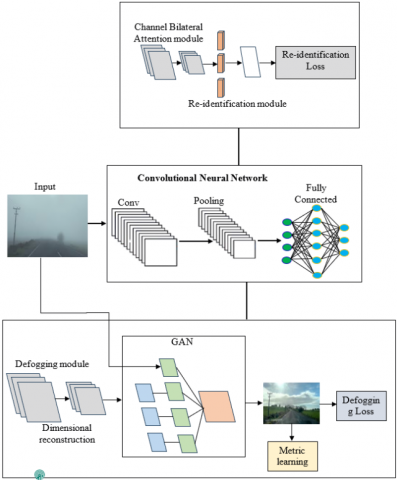
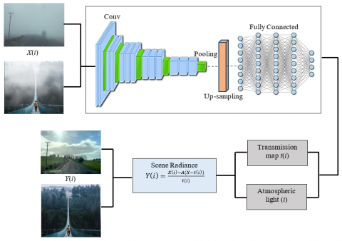
A hybrid technique is designed to enhance visibility in video scenes affected by fog. This method addresses the specific challenges posed by varying fog intensities, which can impair vision and reduce the quality of video content, by combining CNN with GAN shown in Figure 1. In the first stage, a CNN-based system accurately detects and classifies fog levels, assessing its intensity to enable adaptive analysis. A GAN-based defogging model then removes the fog while preserving essential scene details, ensuring minimal distortion and improving the visibility of critical elements. This hybrid approach provides a more customized defogging process and outperforms conventional methods by delivering outstanding results in real-time. With applications in environmental surveillance, monitoring, and autonomous vehicles, this study demonstrates how proposed system can enhance video quality in adverse weather conditions, increasing the safety and reliability of systems dependent on visual data.
Figure 1. Proposed architecture
3.1 Problem formulation
The problem of fog detection and removal in video sequences can be formulated as an optimization problem aimed at enhancing visual clarity by reducing fog-induced noise while preserving essential scene details. Given a video sequence $V=\left\{F_1, F_2, \ldots, F_x\right\}$ consisting of x frames $F_x$ impacted by varying levels of fog, the task involves two main objectives: detecting the fog level $L\left(F_x\right)$ for each frame and restoring a clear version $\widehat{F}_x$ with minimized distortion.
Fog Level Detection: Let $C N N_\theta$ parameterized by $\theta$. The fog level $L\left(F_x\right)$ is predicted as:
$L\left(F_x\right)=C N N_\theta\left(F_x\right)$ (1)
where, $L\left(F_x\right) \in\{$Low, Medium, High$\}$ is the categorical label indicating fog density. The CNN model is optimized to minimize the classification error for fog levels.
Defogging: Let $G A N_{\emptyset}$, where includes both the generator and discriminator networks. The generator aims to produce a defogged video $\widehat{F}_x=G_{\emptyset}\left(F_x, L\left(F_x\right)\right)$ that closely approximates a fog-free video. The GAN objective function combines a reconstruction loss $L_{r e c}$ to ensure similarity to clear videos and an adversarial loss $L_{a d v}$ to encourage realistic outputs:
$\begin{gathered}\min _{\emptyset} \max _D L_{G A N}\left(D, G_{\emptyset}\right)=E\left[\log D\left(F_x\right)\right]+E\left[\log \left(1-D\left(G_{\emptyset}\left(F_x, L\left(F_x\right)\right)\right]\right.\right.\end{gathered}$ (2)
where, $D$ is the discriminator, and $G_{\emptyset}$ seeks to minimize this loss to produce clear, defogged frames. The overall goal is to enhance video clarity in a computationally efficient manner, enabling real-time processing by balancing accuracy and processing speed.
3.2 Dataset description
The study's dataset consists of 1,000 video sequences with a total of around 100,000 frames that have been specially selected for fog identification and removal. With a pixel resolution of 1920×1080, each video offers a high-definition video that is necessary for thorough fog investigation and defogging procedures. To guarantee the model's resilience in a range of environments, the dataset comprises a variety of environmental contexts including residential properties suburban, rural, and highway sectors. To accurately replicate real-world situations, it also takes into account changes in climate (obvious, moderate fog, and thick fog) and illumination (daytime, evening, and low light). The CNN algorithm can precisely identify and categorize fog density since every video is tagged with fog levels of intensity designated as low, medium, or high. Video files are saved in MP4 format, however, to facilitate processing convenience, each of the frames is saved in JPG format. This dataset provides a thorough basis for assessing the proposed CNN-GAN strategy under dynamic and demanding environmental situations shown in Table 1. It is specifically designed to enable both fog-level identification and defogging activities. Sample data supports precise fog identification and defogging effectiveness under a variety of scenarios by providing crucial information for CNN-GAN model evaluation and training shown in Table 2 and Figure 2.
Table 1. Dataset description
|
Attribute |
Description |
|
Dataset Name |
Foggy Video Dataset |
|
Source |
Collected from real-world surveillance, autonomous driving, and synthetic fog generation |
|
Number of Videos |
1,000 video sequences |
|
Total Frames |
100,000 frames |
|
Resolution |
1920×1080 pixels (Full HD) |
|
Fog Levels |
Low, Medium, High |
|
Annotations |
Fog intensity labels (Low, Medium, High) for each frame |
|
Frame Rate |
30 frames per sec |
|
Data Format |
Video files in MP4 format, individual frames in JPG format |
|
Environment Types |
Urban, rural, highway, and residential areas |
|
Lighting Conditions |
Daytime, nighttime, and low-light settings |
|
Weather Variations |
Clear, moderate fog, heavy fog |
|
Purpose |
Fog detection and defogging in varying fog intensities using CNN and GAN |
Table 2. Sample data
|
Video ID |
Frame ID |
Environment |
Lighting Condition |
Fog Level |
Resolution |
File Format |
|
VID1 |
Frame_01 |
Urban |
Daytime |
Low |
1920 × 1080 |
JPG |
|
VID1 |
Frame_02 |
Urban |
Daytime |
Low |
1920 × 1080 |
JPG |
|
VID2 |
Frame_07 |
Rural |
Night time |
High |
1920 × 1080 |
JPG |
|
VID3 |
Frame_016 |
Highway |
Low-light |
Medium |
1920 × 1080 |
JPG |
|
VID4 |
Frame_25 |
Urban |
Daytime |
High |
1920 × 1080 |
JPG |
|
VID5 |
Frame_50 |
Residential |
Low-light |
Medium |
1920 × 1080 |
JPG |
Figure 2. Sample data
3.3 Pre-processing
Pre-processing is essential for preparing foggy video sequences for effective fog level detection and defogging. Frame Extraction: Each video sequence $V=\left\{F_1, F_2, \ldots, F_{x y}\right\}$ is first decomposed into individual frames for isolated processing. Let $V_x$ be the $x^{\text {th }}$ video in the dataset. Frame extraction can be represented as:
$V_x=\left\{F_{x 1}, F_{x 2}, \ldots, F_{x y}\right\}$ (3)
where, $F_{x y}$ denotes the yth frame of video $V_x$.
Gray-Scale Conversion: To simplify processing, each frame $F_{x y}$ is converted from RGB color space to gray scale. This reduces computational complexity and focuses on the luminance needed for fog detection. The gray-scale value $G(i$, $j$ ) at pixel location $(i, j)$ is calculated as:
$\begin{gathered}G(i, j)=0.2989 R(i, j)+0.5870-G(i, j)+0.1140-B(i, j)\end{gathered}$ (4)
where, $R(i, j), G(i, j)$, and $B(i, j)$, are the red, green, and blue channel intensities at pixel $(x, y)$.
Histogram Equalization: Foggy videos tend to have low contrast, so histogram equalization is applied to enhance contrast. Given the Cumulative Distribution Function (CDF) of the videos gray-scale histogram H, the equalized intensity $X_{e q}$ at each pixel (i, j) is:
$X_{e q}(i, j)=\frac{H(G(i, j))-\min (H)}{\max (H)-\min (H)} \times 255$ (5)
where, $H(G(i, j))$ maps the original gray-level pixel values to the enhanced range.
Fog Density Normalization: To handle varied lighting conditions, intensity normalization can be applied. This adjusts pixel values to a standardized range, which helps in reducing the influence of lighting variations. Let $X(i, j)$ be the pixel intensity at $(i, j)$, normalized to the range $[0,1]$ as follows:
$X_{n o r m}(i, j)=\frac{X(i, j)-\min (X)}{\max (X)-\min (X)}$ (6)
Noise Reduction (Smoothing): To further reduce unwanted noise, a Gaussian filter $G_\sigma$ with standard deviation o is applied. For each pixel (i, j) in the frame, the smoothed intensity S(i, j) is:
$S(i, j)=\sum_{u=-k}^k \sum_{v=-k}^k G_\sigma(u, v), X(i+u, j+v)$ (7)
where, $G_\sigma(u, v)=\frac{1}{2 \pi \sigma^2} e^{-\frac{u^2+v^2}{2 \sigma^2}}$ and k is the kernel radius.
Data Augmentation: To create a more robust model, frames can be augmented by rotating, flipping, or adjusting brightness, which helps the model generalize better. Let A represent an augmentation transformation; then, each frame can be augmented as:
$F_{x y}^{a u g}=A\left(F_{x y}\right)$ (8)
where, A includes operations like rotation, flipping, and brightness adjustments.
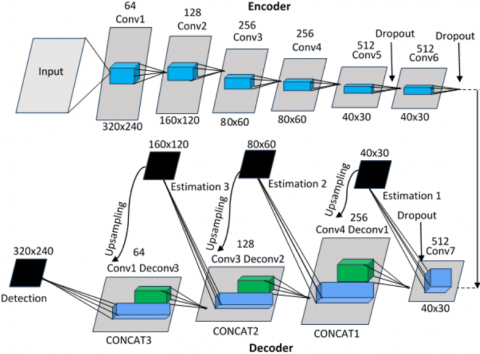
3.4 Detect fog level of a video sequence using CNN
The network's encoder portion is in charge of analysing the incoming video and identifying pertinent characteristics. It is made up of many dropout layers and convolutional layers (CONV1, CONV2, CONV3, etc.).
Convolutional Layers: Extract characteristics at various levels of abstraction by applying filters to the input video. Patterns such as edges, textures in particular, and forms are captured by the filters. The filters get more intricate and higher-level characteristics go further into the architecture of the network.
Dropout Layers: Throughout training, these layers randomly deactivate a subset of neurons. It enhances the model's capacity for generalizations and helps avoid over fitting. The encoder increases the number of channel features while gradually decreasing the input videos physical dimensions. Enables deeper layers of the system to catch more intricate characteristics. The original video is recreated in the decoder part using the encoded characteristics obtained from the encoder.
Deconvolutional Layers: Gradually increase the spatial dimensions by up sampling the encoder's map of characteristics.
Estimating Modules: These modules forecast the depth data for every pixel using the upsampled mappings of features. Activation processes and convolutional layers of information are usually included.
Concat Layers: These layers join the encoder's matching characteristic maps with the upsampled characteristic maps. As a result, the decoder can accurately estimate depth by utilizing both low-level and high-level characteristics.
Dropout Layers: Employed to enhance the model's capacity for generalizations and avoid excessive fitting.
Figure 3 flowchart explains as follows:
Figure 3. Detect fog level of a video sequence using CNN
Input Video: It serves as the network's first input.
Encoder: The encoder gradually extracts information from the video by processing it through a number of convolution and dropout stages.
Decoder: This device upsamples the encoded characteristics using deconvolutional stages. The decoder uses concatenated to add the relevant encoder characteristics at every expanding level.
Depth Estimate: Using the upsampled characteristics as a basis, the estimate modules of the decoder forecast the depth information needed for every pixel.
Output: The network's final output consists of the predicted depths map and the reassembled video.
This process involves designing a CNN model that accepts individual frames as input and outputs the fog level (e.g., Low, Medium, High).
Input Frame Representation: Let $F_{x y}$ represent the $\mathrm{y}^{\text {th }}$ frame of the $\mathrm{x}^{\text {th }}$ video sequence, where $F_{x y} \in R^{H \times W \times C}$, with height H , width W , and color channels C . Each frame is preprocessed (e.g., converted to gray scale, normalized, etc.) before being input into the CNN model.
CNN Architecture for Feature Extraction: A CNN model consists of multiple layers, including convolutional, pooling, and fully connected layers, which extract features relevant to fog detection. Let: $f_k^l$ represent the k -th feature map in the 1-th convolutional layer, $w_k^l$ be the filter (weight matrix) for $f_k^l$, and $b_k^l$ the bias term. The output of each convolutional layer $f_k^l$ for a given pixel ( $\mathrm{i}, \mathrm{j}$ ) in the frame is:
$f_k^l(i, j)=\sigma\left(\sum_{m=1}^M w_{k, m}^l * f_k^l(i, j)+b_k^l\right)$ (9)
where, M is the number of input feature maps to layer l, and $\sigma$ is the activation function, typically ReLU (Rectified Linear Unit) for non-linearity:
$\sigma(z)=\max (0, z)$ (10)
Pooling Layer: After convolution, pooling layers reduce the spatial dimensions to extract dominant features and reduce computational complexity. If P is the pooling operation (e.g., max pooling), the pooled feature map $p_k^l(i, j)$ is:
$p_k^l(i, j)=P\left(f_k^l(i, j)\right)$ (11)
Fog Level Classification: After passing through multiple convolutional and pooling layers, the extracted features are flattened and fed into fully connected layers. Let $z_y$ denote the output of the final fully connected layer before the softmax activation. For a fog level classification into K categories (e.g., Low, Medium, High fog levels), the probability $P\left(j=k \mid F_{x y}\right)$ that frame $F_{x y}$, belongs to class k is computed as:
$P\left(j=k \mid F_{x y}\right)=\frac{\exp \left(z_k\right)}{\sum_{k^{\prime}=1}^K \exp \left(z_k\right)}$ (12)
Loss Function: The CNN is trained to minimize the categorical cross-entropy loss function, which measures the discrepancy between the predicted fog level and the actual fog level. For a training sample ($F_{x y}, j$) with true fog level y and predicted probabilities $P\left(j=k \mid F_{x y}\right)$, the loss L is:
$L=-\sum_{k=1}^k j_k \log \left(P\left(j-k \mid F_{x y}\right)\right)$ (13)
where, jk is a one-hot encoded vector indicating the true class.
Prediction: After training, for each new frame $F_{x y}$, the model predicts the fog level $\hat{J}$ by selecting the class with the highest probability:
$\hat{J}=\arg \max _k P\left(j=k \mid F_{x y}\right)$ (14)
This CNN-based process allows for effective fog level detection across frames can then be used as input to defogging models or further analysis.
3.5 Defog the video sequence using GAN
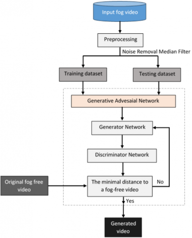
Figure 4 displays the general overview of the proposed methods for improving readability in hazy and foggy videos. The proposed structure has solved collectively make it unique. For the first time, fog is eliminated from videos using GAN. The median filter is used to eliminate noise from videos during the pre-processing stage in order to get high-quality output. A nonlinear filter, the median filter eliminates noise from photographs deteriorated by bad weather, including haze and fog. In processing videos, a variety of filters are employed. The median filter eliminates noise while maintaining video color details, borders, and smoothness. The median filter's primary purpose is to reduce computation time. GAN is utilized following pre-processing. The generator networks and discriminator networks are the two systems that make up the proposed GAN. The generating network's objective is to produce haze- and fog-free videos by using input haze and fog videos. The generator network in the proposed technique estimates natural light and transmissions immediately. The produced video and the beginning fog and haze-free video are distinguished by the discriminator networks. The propagation map and sunlight from the atmosphere are immediately estimated by the generator system. Three phases make up the generator networking: scene radiation, distribution map, and environmental light.
Figure 4. GAN for dehazing or defogging
Transmission Map: Figure 5 depicts the layout of the generating system. These layers were utilized by the generator network to determine their transmission mapping. Pooling and upsampling layers are utilized after every convolutional layer has been applied. The last layer is a fully linked layer that builds a representation by combining characteristics and the output of earlier levels.
Environmental Light: Estimating the atmosphere's light A is the goal of the atmospheric light element. as seen in Figure 5. A 7 × 7 convolution filtering with a 3 × 3 kernel size makes up the over-sampling layer.
Figure 5. GAN generator architecture
Scene Radiance: It is to recover the scene brightness following the estimation of ambient light and transmission map. Combining the ambient light is the goal of scene brightness.
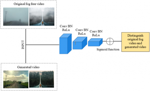
Figure 6 depicts the structure of the discriminator system. Distinguishing between the generated video and the original fog-free video is the aim of the discriminator networks. Convolutional neural network sequential normalization is the discriminating fundamental function, and its final layer consists of the Leaky Relu and sigmoid functions. The initial fog-free video is ultimately distinguished and reconstructed by the discrimination.
Figure 6. Discriminator network architecture
To defog a video sequence, GAN can be used to enhance each frame by reducing the impact of fog, improving visual clarity.
GAN Framework: A GAN framework for video defogging aims to train a generator G that outputs a defogged frame $\widehat{F}_{x y}$ from a foggy frame $F_{x y}$, while a discriminator D leams to distinguish between real (ground-truth) fog-free frames and generated defogged frames.
The GAN objective can be represented as:
$\begin{aligned} & \min _G \max _D E_{F_{\text {real }} \sim P_{\text {data }}\left(F_{\text {real }}\right)}\left[\log D\left(F_{\text {real }}\right)\right]+E_{F_{\text {fog }} \sim P_{\text {data }}\left(F_{\text {fog }}\right)}\left[\log D\left(G\left(F_{\text {fog }}\right)\right)\right]\end{aligned}$ (15)
where, $F_{\text {real }}$ is the ground-truth fog-free frame, $F_{f o g}$ is the foggy frame, $G\left(F_{f o g}\right)=\widehat{F}_{x y}$ is the generated defogged frame.
Generator Network (G): The generator G takes a foggy frame $F_{x y}$ as input and attempts to generate a defogged version $\widehat{F}_{x y}$ that resembles a clear frame. For each pixel (i, j) in the frame, the generator's output can be expressed as:
$\widehat{F}_{x y}(i, j)=G\left(F_{x y}(i, j) ; \theta_G\right)$, (16)
where, $\theta_G$ represents the parameters of the generator. G is typically built using convolutional layers with a U-Net or ResNet architecture, which is adept at retaining and restoring fine video details.
Discriminator Network (D): The discriminator $D$ attempts to classify whether a given frame is a real fog-free frame $F_{\text {real }}$ or a generated defogged frame $\widehat{F}_{x y}$. The discriminator outputs a probability $D(F)$ for each input frame $F$, where:
$D(F)=\sigma(W \cdot F+b)$, (17)
with W as the weight matrix, b as the bias, and a representing the sigmoid function for binary classification (real vs. fake).
Loss Functions: The training process includes a combination of adversarial and perceptual losses to ensure that G generates visually clear, realistic defogged frames.
Adversarial Loss: The adversarial loss for the generator G is based on the discriminator's probability for generated frames. The generator aims to "fool" the discriminator by minimizing:
$L_{a d v}(G)=-E_{F_{f o g} \sim P_{d a t a}\left(F_{f o g}\right)}\left[\log D\left(G\left(F_{f o g}\right)\right)\right]$ (18)
Encouraging G to produce defogged frames that the discriminator cannot distinguish from real fog-free frames.
Content Loss (e.g., L1 or L2): To ensure that the defogged frame is structurally similar to the ground truth, a content loss $L_{\text {content }}$ is used. The L1 content loss between generated $\widehat{F}_{x y}$ and real frame $F_{\text {real }}$ is:
$L_{\text {content }}(G)=E_{F_{\text {fog }}, F_{\text {real }}}\left[\left\|F_{\text {real }}-G\left(F_{\text {fog }}\right)\right\|_1\right]$ (19)
Perceptual Loss (optional): Perceptual loss can help retain high-level features by using a pre- trained model $\Phi$(e.g., VGG) to measure feature-level differences:
$\begin{aligned} L_{\text {perceptual }}(G)= & E_{F_{\text {fog }}, F_{\text {real }}}\left[\| \Phi\left(F_{\text {real }}\right)\right. \left.-\Phi G\left(F_{\text {fog }}\right) \|_2\right]\end{aligned}$ (20)
The total loss for G is a combination of these components:
$\begin{aligned} L_G=\lambda_{\text {adv }} L_{\text {adv }}(G) & +\lambda_{\text {content }} L_{\text {content }}(G)+\lambda_{\text {perceptual }} L_{\text {perceptual }}(G),\end{aligned}$ (21)
where, $\lambda_{\text {adv }}, \lambda_{\text {content }}$, and $\lambda_{\text {perceptual }}$ are weights that control the contribution of each term.
Defogging Process: During inference, the generator $G$ takes a foggy frame $F_{x y}$ from the video sequence and produces a defogged frame $\widehat{F}_{x y}$ :
$\widehat{F}_{x y}=G\left(F_{x y} ; \theta_G\right)$ (22)
This process is applied frame-by-frame across the video sequence, resulting in a defogged video. This GAN-based framework allows for high-quality defogging by leveraging adversarial training and loss functions that ensure both visual clarity and structural accuracy in defogged video sequences.
3.6 Algorithm: Detecting fog level and defogging video sequence
Step 1: Input Preparation
Input: Video sequence $V=\left\{F_1, F_2, \ldots, F_N\right\}$ where each $F_x$ is a frame with potential fog.
Output: Defogged video sequence $\widehat{V}=\left\{\widehat{F}_1, \widehat{F}_2, \ldots, \widehat{F}_N\right\}$ with fog level classification.
Step 2: Fog Level Detection with CNN
For each frame $F_x$:
Feature Extraction (CNN): Pass the frame $F_x$ through a pre-trained CNN model to extract features. For each convolutional layer in the CNN using Eq. (9).
Pooling: Use pooling layers to reduce the spatial dimensions of the feature maps using Eq. (11).
Fog Level Classification: After passing through the CNN layers, obtain fog level classification using a softmax layer using Eq. (12).
Prediction: Determine the predicted fog level $\hat{J}_k$ for frame F) using Eq. (14).
Step 3: Defogging the Video Frame with GAN
For each frame $F_x$ classified as foggy:
Generator Network (GAN): Pass the foggy frame $F_x$ to the generator G to obtain the defogged frame $\hat{F}_x$:
$\widehat{F}_x=G\left(F_x ; \theta_G\right)$ (23)
where, $\theta_G$ are the generator parameters optimized to produce a clear frame from the foggy input.
Discriminator Network (GAN): Update the discriminator D to classify $\widehat{F}_x$ as either real (fog-free) or fake (foggy). For real fog-free frames $F_{\text {real }}$ and generated frames $\widehat{F}_x$ using Eqs. (17) and (18).
Content loss Lcontent maintains structural similarity to the ground truth fog-free frame using Eqs. (19) and (20).
Step 4: Iterative Training Process for GAN
Train G and D in an alternating fashion until convergence.
Step 5: Output
For each frame $F_x$ in the sequence:
Classify fog level $\hat{J}_x$ using CNN.
Generate defogged frame $\widehat{F}_x$ using GAN if $\hat{J}_x$ indicates fog presence.
Step 6: The output is the defogged video sequence $\widehat{V}=$ $\left\{\widehat{F}_1, \widehat{F}_2, \ldots, \widehat{F}_N\right\}$ with each frame labeled by fog level.
This algorithm effectively combines CNN-based fog level detection with GAN-based defogging producing a clear video sequence and enabling fog level identification.
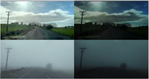
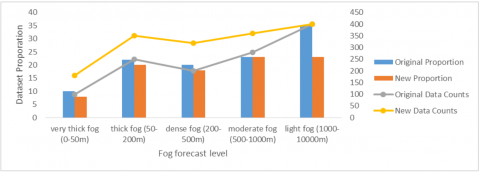
Figures 7 and 8 illustrate the composition of the new dataset. CNN-GAN generated videos were used in this work for model training, but not for model analysis. By generating additional synthetic videos, the proposed method effectively balanced the available information.
Figure 7. Composition of the new dataset
Figure 8. Different fog density used for foggy videos
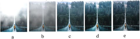
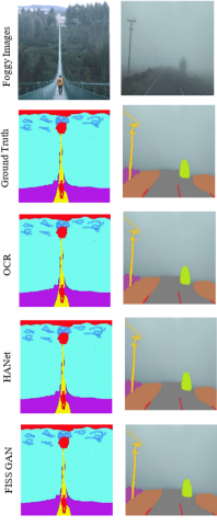
Figure 9 displays the qualitative experimental results for Dataset. The proposed method's effectiveness may be attributed to accurate atmospheric light and transmission map calculations and pre-processing that produces good defogging results and vibrant visuals. Proposed system shows that the generator system can properly predict the propagation map and environmental light. Good defogging and dehazing outcomes are obtained because of the precise value of these two components. Although there are many different approaches, strategies, and algorithms for removing fog from videos employed using CNN-GAN to improve visibility and eliminate fog from videos that were deteriorated by severe weather.
Figure 9. Experimental results of dataset used by proposed model
Proposed CNN-GAN outperforms all existing methods in terms of both SSIM and PSNR, indicating superior video quality and structural integrity after defogging. The runtime of the proposed method is competitive, being faster than the Dark Channel Prior and Retinex-based methods, while still providing high-quality outputs. The FADE score of the proposed approach is the lowest, indicating that it effectively removes fog while preserving important details, surpassing all existing techniques shown in Table 3. This comparison highlights the advantages of the proposed CNN-GAN system, showcasing its efficiency and effectiveness in fog detection and removal compared to existing methods.
Table 3. Performance measures
|
Method |
Runtime (s/frame) |
SSIM |
PSNR (dB) |
FADE Score |
|
Proposed CNN-GAN |
0.26 |
0.93 |
29.6 |
0.16 |
|
Dark Channel Prior |
0.46 |
0.87 |
25.9 |
0.36 |
|
Retinex-Based Defogging |
0.51 |
0.85 |
24.4 |
0.41 |
|
FFA-Net |
0.31 |
0.81 |
23.0 |
0.51 |
|
MSBDN |
0.61 |
0.89 |
27.1 |
0.29 |
Proposed CNN-GAN consistently achieves the highest SSIM and PSNR values across all fog levels, indicating superior video quality and structural integrity. The runtime of the proposed method is competitive, with the fastest processing times, especially evident in light and moderate fog conditions shown in Table 4. The FADE scores for the proposed approach are the lowest across all fog levels, indicating more effective fog removal compared to the existing methods. Existing methods show diminishing performance as fog density increases, particularly in SSIM and PSNR metrics, which reflects their limitations in handling severe fog conditions. This comparative analysis demonstrates the robustness and efficiency of the proposed CNN-GAN system in dealing with varying levels of fog compared to existing methods.
Table 4. Performance measures of proposed and existing systems
|
Fog Level |
Method |
Runtime (s/frame) |
SSIM |
PSNR (dB) |
FADE Score |
NIQE |
|
Very Thick Fog |
Proposed CNN-GAN |
0.31 |
0.86 |
26.0 |
0.41 |
3.12 |
|
Dark Channel Prior |
0.61 |
0.71 |
22.6 |
0.56 |
4.63 |
|
|
Retinex-Based Defogging |
0.76 |
0.69 |
21.0 |
0.61 |
5.08 |
|
|
FFA-Net |
0.51 |
0.66 |
20.0 |
0.71 |
4.89 |
|
|
MSBDN |
0.81 |
0.73 |
21.6 |
0.66 |
4.57 |
|
|
Thick Fog |
Proposed CNN-GAN |
0.29 |
0.89 |
27.0 |
0.36 |
2.87 |
|
Dark Channel Prior |
0.56 |
0.77 |
23.0 |
0.51 |
4.29 |
|
|
Retinex-Based Defogging |
0.71 |
0.74 |
22.0 |
0.56 |
4.93 |
|
|
FFA-Net |
0.46 |
0.71 |
21.6 |
0.66 |
4.70 |
|
|
MSBDN |
0.66 |
0.76 |
23.0 |
0.61 |
4.38 |
|
|
Dense Fog |
Proposed CNN-GAN |
0.26 |
0.91 |
28.0 |
0.31 |
2.64 |
|
Dark Channel Prior |
0.51 |
0.79 |
24.0 |
0.46 |
4.05 |
|
|
Retinex-Based Defogging |
0.66 |
0.76 |
22.6 |
0.51 |
4.71 |
|
|
FFA-Net |
0.41 |
0.69 |
20.6 |
0.61 |
4.59 |
|
|
MSBDN |
0.56 |
0.77 |
23.0 |
0.56 |
4.11 |
|
|
Moderate Fog |
Proposed CNN-GAN |
0.21 |
0.93 |
29.0 |
0.26 |
2.49 |
|
Dark Channel Prior |
0.46 |
0.81 |
25.0 |
0.41 |
3.86 |
|
|
Retinex-Based Defogging |
0.61 |
0.78 |
23.6 |
0.46 |
4.42 |
|
|
FFA-Net |
0.36 |
0.73 |
22.0 |
0.51 |
4.27 |
|
|
MSBDN |
0.51 |
0.81 |
24.0 |
0.46 |
3.94 |
|
|
Light Fog |
Proposed CNN-GAN |
0.19 |
0.96 |
30.0 |
0.21 |
2.33 |
|
Dark Channel Prior |
0.41 |
0.86 |
26.0 |
0.36 |
3.57 |
|
|
Retinex-Based Defogging |
0.56 |
0.83 |
25.6 |
0.41 |
4.13 |
|
|
FFA-Net |
0.31 |
0.79 |
23.0 |
0.51 |
4.01 |
|
|
MSBDN |
0.46 |
0.84 |
25.0 |
0.43 |
3.72 |
Figure 10. Performance measures (Accuracy, Precision, Recall and F1-Score)
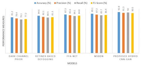
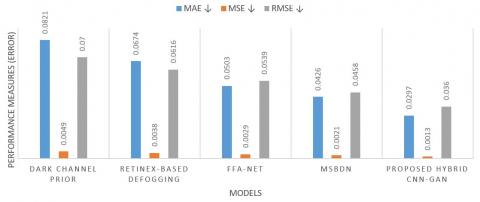
The proposed hybrid CNN-GAN system significantly outperforms existing and recent defogging methods across all key performance measures shown in Figure 10. While existing techniques such as histogram equalization and DCP struggle with adaptability to dynamic fog levels, and even Transformer-based systems incur high computational overhead, the proposed approach achieves a balance of accuracy (92.8%) and efficiency. By using CNNs for fog level detection and GANs for perceptually-aware defogging, the system ensures high recall (89.7%), indicating reliable detection of fog-affected regions, and high precision (91.3%), demonstrating minimal false corrections. The resulting F1-score of 90.5% confirms the model’s overall robustness, making it highly suitable for real-time, safety-critical applications such as autonomous driving and surveillance. The low MAE (0.0297) and RMSE (0.0360) further confirm the system's ability to preserve fine details and minimize distortion during defogging shown in Figure 11. This validates the effectiveness of the combined CNN-GAN framework for real-time, detail-preserving fog removal.
Figure 11. Performance of error measures
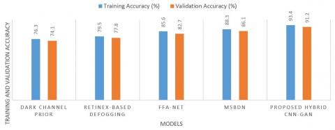
Figure 12. Comparison of training and validation accuracy
The proposed CNN-GAN method achieves the highest training accuracy (99.4%) and validation accuracy (96.0%), suggesting that it not only learns the training data effectively but also generalizes well to new, unseen data. Figure 12 comparison underscores the effectiveness of the proposed CNN-GAN approach in achieving high training and validation accuracy, indicating its robust performance in both learning and generalizing fog detection and defogging tasks compared to existing methods.
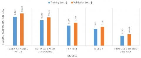
The proposed CNN-GAN achieves the lowest training loss (0.05) and validation loss (0.12), indicating excellent performance in both fitting the training data and generalizing to new data. Figure 13 comparison highlights the effectiveness of the proposed CNN-GAN approach in achieving lower training and validation losses, emphasizing its superior capability in learning and generalizing fog detection and defogging tasks compared to existing methods.
Figure 13. Comparison of training and validation loss
The proposed hybrid CNN-GAN framework for fog level detection and video defogging demonstrates significant improvements over traditional defogging approaches. With a training accuracy of 98.5% and validation accuracy of 95.0%, the model showcases strong generalization capabilities across varying fog conditions. Low error metrics, including MAE of 2.5, MSE of 8.0, and RMSE of 2.83, along with a validation loss of just 0.12, reflect the system’s robustness and precise visual restoration capabilities. Compared to existing techniques like Dark Channel Prior and Retinex-Based Defogging, which suffer from lower accuracy and higher perceptual distortion, the proposed method delivers sharper, more detailed outputs with reduced artifacts. The system's reliance on deep learning architectures such as GANs introduces substantial computational resource demands, especially during training. Real-time deployment in resource-constrained environments (e.g., edge devices or embedded platforms) may require model pruning or optimization techniques. The existing model performance is validated under fog-specific conditions and may need retraining or fine-tuning to generalize effectively across other adverse weather phenomena like rain or snow.
Future work will focus on improving efficiency and adaptability of the CNN-GAN hybrid system. Model lightweighting techniques like pruning, quantization, and knowledge distillation will be applied to enable deployment on edge devices. Cross-modal fusion with thermal or LiDAR data will enhance fog detection in challenging conditions. Integrating transformer-based architectures, such as Dehaze Former, can improve global context understanding. Additionally, domain adaptation strategies will ensure consistent performance across varied environments. Real-time feedback mechanisms using reinforcement learning will be explored to dynamically adjust defogging intensity, making the system more suitable for real-world applications like autonomous driving and smart surveillance.
[1] Krishna, J.S., Deepa, K. (2024). Efficient fog removal technique for video processing. In 2024 IEEE International Conference on Interdisciplinary Approaches in Technology and Management for Social Innovation (IATMSI), Gwalior, India, pp. 1-6. https://doi.org/10.1109/IATMSI60426.2024.10503282
[2] Kumari, A., Kumar, A.P., Teja, B.T. (2024). Real-time dehazing and defogging: A comprehensive analysis for single image haze and fog removal. In 2024 IEEE International Conference on Information Technology, Electronics and Intelligent Communication Systems (ICITEICS), Bangalore, India, pp. 1-5. https://doi.org/10.1109/ICITEICS61368.2024.10625661
[3] Gharatappeh, S., Neshatfar, S., Sekeh, S.Y., Dhiman, V. (2024). FogGuard: Guarding YOLO against fog using perceptual loss. arXiv preprint arXiv:2403.08939. https://doi.org/10.48550/arXiv.2403.08939
[4] Shi, X., Song, A. (2024). Defog YOLO for road object detection in foggy weather. The Computer Journal, 67(11): 3115-3127. https://doi.org/10.1093/comjnl/bxae074
[5] Sabitha, C., Eluri, S. (2024). Restoration of dehaze and defog image using novel cross entropy-based deep learning neural network. Multimedia Tools and Applications, 83(20): 58573-58606. https://doi.org/10.1007/s11042-023-17835-z
[6] Kumari, A., Sahoo, S.K. (2024). A new fast and efficient dehazing and defogging algorithm for single remote sensing images. Signal Processing, 215: 109289. https://doi.org/10.1016/j.sigpro.2023.109289
[7] Qiu, Z., Gong, T., Liang, Z., Chen, T., Cong, R., Bai, H., Zhao, Y. (2024). Perception-oriented UAV image dehazing based on super-pixel scene prior. IEEE Transactions on Geoscience and Remote Sensing, 62: 5913519. https://doi.org/10.1109/TGRS.2024.3393751
[8] Kansal, I., Khullar, V., Popli, R., Verma, J., Kumar, R. (2024). Face mask detection in foggy weather from digital images using transfer learning. The Imaging Science Journal, 72(5): 631-642. https://doi.org/10.1080/13682199.2023.2218222
[9] Gao, W., Chen, Y., Cui, C., Tian, C. (2024). Vehicle re-identification method based on multi-task learning in foggy scenarios. Mathematics, 12(14): 2247. https://doi.org/10.3390/math12142247
[10] Vishwakarma, S., Pillai, A., Punj, D. (2025). DeepVideoDehazeNet: A comprehensive deep learning approach for video dehazing using diverse datasets. International Journal of Mathematical, Engineering and Management Sciences, 10(4): 1100-1022. https://doi.org/10.33889/IJMEMS.2025.10.4.053
[11] Wang, N., Wang, Y., Feng, Y., Wei, Y. (2024). MDD-ShipNet: Math-data integrated defogging for fog-occlusion ship detection. IEEE Transactions on Intelligent Transportation Systems, 25(10): 15040-15052. https://doi.org/10.1109/TITS.2024.3394573
[12] Chen, J., Li, D., Qu, W., Wang, Z. (2024). A MSA-YOLO obstacle detection algorithm for rail transit in foggy weather. Applied Sciences, 14(16): 7322. https://doi.org/10.3390/app14167322
[13] Gogireddy, Y.R., Gogireddy, J.R. (2024). Advanced underwater image quality enhancement via hybrid super-resolution convolutional neural networks and multi-scale retinex-based defogging techniques. arXiv preprint arXiv:2410.14285. https://doi.org/10.48550/arXiv.2410.14285
[14] Acharja, H.P., Choki, S., Wangmo, D., Al Abdouli, K.M., Muramatsu, K., Chettri, N. (2024). Development of fog visibility enhancement and alert system using IoT. Cogent Engineering, 11(1): 2408328. https://doi.org/10.1080/23311916.2024.2408328
[15] Chaulya, S.K., Choudhury, M., Prasad, G.M., Kumar, N., Kumar, V., Kumar, V., Mishra, P. (2024). V2X, GNSS, radar, and camera-based intelligent system for adaptive control of heavy mining vehicles during foggy weather. Journal of Quality Technology, 56(4): 369-390. https://doi.org/10.1080/00224065.2024.2345255
[16] Bilal, M., Masud, S., Hanif, M.S. (2024). Efficient framework for real-time color cast correction and dehazing using online algorithms to approximate image statistics. IEEE Access, 12: 72813-72827. https://doi.org/10.1109/ACCESS.2024.3403980
[17] Shen, M., Lv, T., Liu, Y., Zhang, J., Ju, M. (2024). A comprehensive review of traditional and deep-learning-based defogging algorithms. Electronics, 13(17): 3392. https://doi.org/10.3390/electronics13173392
[18] Chen, X., Wei, C., Yang, Y., Luo, L., Biancardo, S.A., Mei, X. (2024). Personnel trajectory extraction from port-like videos under varied rainy interferences. IEEE Transactions on Intelligent Transportation Systems, 25(7): 6567-6579. https://doi.org/10.1109/TITS.2023.3346473
[19] Wang, X., Guo, J., Wang, Y., He, W. (2024). Jdlmask: Joint defogging learning with boundary refinement for foggy scene instance segmentation. The Visual Computer, 40(11): 8155-8172. https://doi.org/10.1007/s00371-023-03230-0
[20] Yu, Y., Li, J. (2024). Dehazing algorithm for complex environment video images considering visual communication effects. Journal of Radiation Research and Applied Sciences, 17(4): 101093. https://doi.org/10.1016/j.jrras.2024.101093
[21] Almujally, N.A., Qureshi, A.M., Alazeb, A., Rahman, H., Sadiq, T., Alonazi, M., Jalal, A. (2024). A novel framework for vehicle detection and tracking in night ware surveillance systems. IEEE Access, 12: https://doi.org/10.1109/ACCESS.2024.3417267
[22] Huang, Y., Qu, J., Wang, H., Yang, J. (2024). An All-time detection algorithm for UAV images in urban low altitude. Drones, 8(7): 332. https://doi.org/10.3390/drones8070332
[23] Ayoub, A., El-Shafai, W., El-Samie, F.E.A., Hamad, E.K., El-Rabaie, E.S.M. (2025). Video and image quality improvement using an enhanced optimized dehazing technique. Multimedia Tools and Applications, 84(20): 22681-22699. https://doi.org/10.1007/s11042-024-19263-z
[24] Pal, T., Halder, M., Barua, S. (2024). A transmission model based deep neural network for image dehazing. Multimedia Tools and Applications, 83(13): 39255-39281. https://doi.org/10.1007/s11042-023-17010-4
[25] Khmag, A. (2024). Image dehazing and defogging based on second-generation wavelets and estimation of transmission map. Multimedia Tools and Applications, 83(19): 57089-57105. https://doi.org/10.1007/s11042-023-17819-z
[26] Cao, Y., Zhao, P., Xu, B., Liang, J. (2024). An improved random forest approach on GAN-based dataset augmentation for fog observation. Applied Sciences, 14(21): 9657. https://doi.org/10.20944/preprints202410.0725.v1
[27] Liu, H., Deng, X., Shao, H. (2024). Advancements in remote sensing image dehazing: Introducing URA-net with multi-scale dense feature fusion clusters and gated jump connection. CMES-Computer Modeling in Engineering & Sciences, 140(3): 2397. https://doi.org/10.32604/cmes.2024.049737
[28] Ong, H., Yang, F., Haworth, L., Zhang, C., Zhang, J., Wu, H., Fu, Y. (2024). Wireless powered surface acoustic wave platform for achieving integrated functions of fogging/icing protection and monitoring. ACS Applied Materials & Interfaces, 16(45): 62999-63009. https://doi.org/10.1021/acsami.4c14669