Real-Time and Accurate Pupil Detection Based Retro-Oriented Mind and Ellipse Trend Analysis

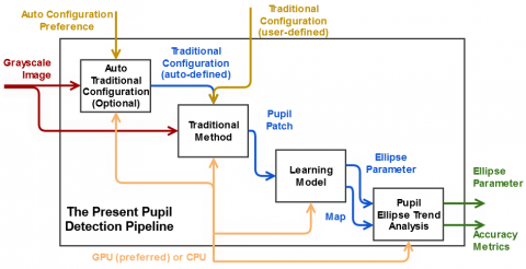
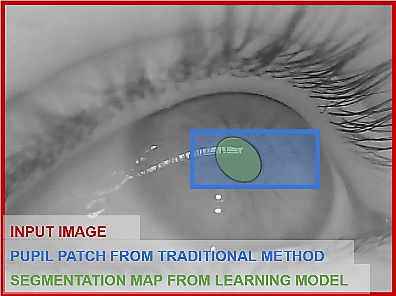
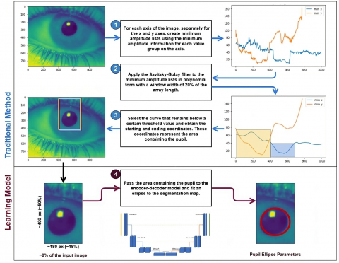
The system's architecture comprises three key components: i) the traditional method, ii) the learning model within the scope of ROM, and lastly iii) PETA step. The traditional method process requires a grayscale input image and a configuration (thresholding etc.) to be used in finding pupil patches and exports a patch that will be in reduced resolution compared to the input image. Subsequently, learning model receives the patch and uses it to segment pupil area within the patch. Next, fitting an ellipse to segmentation map is actualized here. The PETA component comes into play by calculating accuracy metrics using the ellipse parameters and potentially making corrections if necessary. For an illustrative depiction of this architecture, given Figure 1, which represents the system as a top-level activity within an SADT (Structured Analysis and Design Technique) diagram [67].

image003.png

image004.png

Figure 1. The general structure of the present study as a top-level activity of SADT diagram and the visualized result according to the pupil patch received from the traditional method and ellipse parameters calculated by the model step

It's essential to acknowledge that manually determining the traditional method configuration may lead to the patch containing insufficient or no pupil region when the image contains a pupil. This negatively impacts detection accuracy.  To address this issue, an optional mechanism has been added to the system. This mechanism works at a desired time interval (e.g., every second) in a separated thread. It takes the input image which it receives at the end of the time interval and actively seeks to identify the traditional method configuration that optimally suits the given image. Thus, it tries to provide reliable and precise results.

2.1 Traditional method

The causes of inaccurate results in amplitude-based traditional methods are more predictable compared to edge-based and edge-amplitude-hybrid traditional methods. Consequently, amplitude-based traditional methods may allow the user to define configuration or initialization settings in a more controlled manner. Believing in the potential success of amplitude-based methods when used correctly, we propose an amplitude-based method for the traditional method part of the study. The proposed method has three sequential subparts:

(i) Finding Minima Pixel Sequences: The lowest amplitudes are obtained in each row for the x-axis and in each column for the y-axis. They are collected in a sequence form as given in the expression below. I_ij denotes pixel values of a received image. Since the sequences were created using all rows or columns of the image, each index of these sequences corresponds to a coordinate point, and the sequences include high-variance noise.

${{S}_{row}}=\left[ \begin{matrix}   \min \left( {{I}_{1,1}},{{I}_{1,2}},\cdots ,{{I}_{1j}} \right)  \\   \min \left( {{I}_{2,1}},{{I}_{2,2}},\cdots ,{{I}_{2j}} \right)  \\   \vdots   \\   \min \left( {{I}_{i,1}},{{I}_{i,2}},\cdots ,{{I}_{ij}} \right)  \\ \end{matrix} \right],\\ {{S}_{col}}=\left[ \begin{matrix}   \min \left( {{I}_{1,1}},{{I}_{2,1}},\cdots ,{{I}_{i1}} \right)  \\   min\left( {{I}_{1,2}},{{I}_{2,2}},\cdots ,{{I}_{i2}} \right)  \\   \vdots   \\   min\left( {{I}_{1,j}},{{I}_{2,j}},\cdots ,{{I}_{ij}} \right)  \\\end{matrix} \right]~~$                 (1)

(ii) Noise Reduction: To mitigate the noise present in the minima sequences, the Savitzky-Golay (SG) method was applied as a smoothing filter [68]. The filter fits a local polynomial to a window of adjacent data points and then uses the coefficients of this polynomial to compute the smoothed value at the center of the window. Filtered output of i^th sample ${{\hat{S}}_{i}}$ is calculated by a weighted summation of input signal neighbors. The coefficients ${{C}_{j}}~$are determined by solving the least squares polynomial fitting problem .for each window. In SG method, window length parameter (2L+1) is individually set to 20% of the length of each sequence.

${{\hat{S}}_{i}}=\underset{j=-L}{\overset{L}{\mathop \sum }}\,{{C}_{j}}\times {{S}_{i+j}}$                       (2)

(iii) Patch Selection: Patch selection is carried out using the smoothed sequences. The configuration settings to be taken from the user or to be defined by auto traditional method configuration mechanisms are used in this step. Three parameters, each associated with a function taking a sequence as input, govern this step: THM for thresholding, PFX (Pupil Founder X) for the x-axis sequence, and PFY (Pupil Founder Y) for the y-axis sequence.

Table 1. THM functions to be used for the selection of threshold value. A value calculated by a THM function is used for sequences of x and y pair of an input image

TH1(S)=max(S)-std(S)	TH2(S)=(MMM×0.66)+min(S)
TH3(S)=max(avg(S), MPM/2)	TH4(S) = avg (S)
TH5(S)=min(avg(S), MPM /2)	TH6(S)=(MMM×0.33)+min(S)
TH7(S)=(avg(S)+min(S))/2	TH8(S)=min(S)+std(S)
where MPM = max(S)+min(S), MMM = max(S)–min(S)

By using a function from THM function list in Table 1, threshold values are defined dynamically for each denoised minima sequence. THM functions and equations taking a sequence shown as S are the below, roughly from highest to lower amplitude values.

Following the smoothing of the minima sequences, the process continues with the application of PFX and PFY to the x-axis and y-axis sequences, respectively. There are a total of five distinct functions, collectively referred to as Pupil Founder (PF) functions, which can be chosen for PFX or PFY. ${{G}_{k}}$  expression is intended for use in relevant functions can be calculated as follows:

${{G}_{k}}=\{{{s}_{i}}|~{{s}_{i}}<\tau ,{{s}_{i+1}}<\tau ,~....,{{s}_{i+n}}<\tau \}$                      (3)

where, ${{G}_{k}}$ represents the grouping of consecutive sequence elements, and ${{s}_{i}}$, ${{s}_{i+1}}$, …,${{s}_{i+n}}$ are the elements of the sequence. The condition, s<$\tau$ is applied to each element in the group, ensuring that they are all smaller than the threshold value $\tau$.

1- Median First (MF): It selects the part closest to the middle index under the threshold of the sequence on the relevant axis. It can be calculated as in Eq. (4):

${{P}_{MF}}=~\text{argmi}{{\text{n}}_{\text{k}}}\left( \text{min}\left( \left| {{G}_{i}}-M\left| , \right|{{G}_{i+1}}-M\left| ,...,~ \right|{{G}_{i+n}}-M \right| \right) \right)$                  (4)

where, M represents the median index of the S array. Accordingly, MF is useful when the objective is to position the pupil near the center of the sequence along the relevant axis. This option can be particularly useful in places where the experimental procedure is well-defined, such as laboratory environments.

2- Max Depth (MD): MD chooses the segment with the lowest amplitude value from the parts under the threshold on the relevant axis. The equation is given in Eq. (5) and it is particularly useful when the pupil is known to exhibit the darkest amplitude. This option carries the potential of obtaining a patch size smaller than expected by preventing the inclusion of other small objects besides the pupil in the patch scope in experimental or in-house environments.

${{P}_{MD}}=\text{argma}{{\text{x}}_{k}}\left| \min \left( {{G}_{k}} \right)-~\tau  \right|$                (5)

3- Max Length (ML): ML selects the segment with the highest number of elements among those below the threshold on the axis in use. This function given in Eq. (6) is suitable when the pupil is known to be larger than other dark areas.

${{P}_{ML}}=\text{argma}{{\text{x}}_{\text{k}}}\left( \left| {{G}_{k}} \right| \right)$                      (6)

4- Max of Length and Depth Product (LD): LD assigns a score to the parts under the threshold on the axis it is used and selects the part with the highest score. Score to be calculated with the expression is the product of the number of elements of the part and its absolute distance from the threshold level of the lowest amplitude. Hereby, this function given in Eq. (7) can be used when the pupil is known to be darker or larger.

Thus, it can ensure that the dark but small areas outside the pupil and the areas that are not as dark as the pupil but occupy a large area are not included in the patch.

${{P}_{LD}}=\text{argma}{{\text{x}}_{\text{k}}}\left( \left| {{G}_{k}} \right|*\left| \min \left( {{G}_{k}} \right)-~\tau  \right| \right)$                      (7)

image007.png

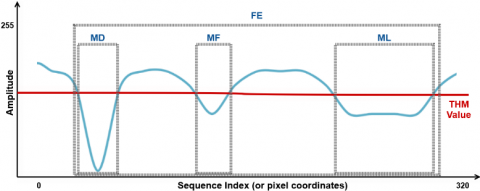
Figure 2. A denoised minima sequences for x-axis and different patches selected by PF functions

(Basically, these functions try to select one segment between parts under the threshold value)

image008.jpg

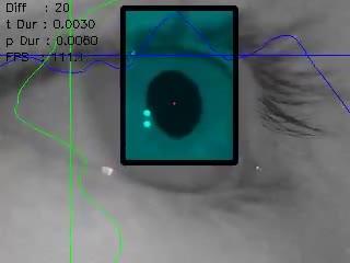
Figure 3. An example of the selected patch with randomly defined configurations

5- First and End (FE): FE selects the entire area between the first and last indices under the threshold in the axis on which it is used. The equation given in Eq. (8) is beneficial in cases where perceiving the pupil based on amplitude information alone is challenging and may result in an enlarged patch size. In general, this should be the last alternative to be chosen, indicating the need for pre-experimental preparation for other options to work effectively. However, in an environment where pupil in-formation is adequately detected, it still has the potential to produce results like the previous functions.

${{P}_{FE}}=\left\{ {{s}_{n}},{{s}_{n+1}},\cdots ,{{s}_{m}} \right\}$                      (8)

$\text{where},~n=\min \text{ }\!\!\{\!\!\text{ }j~\text{ }\!\!|\!\!\text{ }{{s}_{j}}<~\tau \}\text{ }\!\!~\!\!\text{ and }\!\!~\!\!\text{ }m=\max \text{ }\!\!\{\!\!\text{ }j~\text{ }\!\!|\!\!\text{ }{{s}_{j}}<~\tau \}\}$.

These selections except for LD have been shown via an example minima sequence in Figure 2. Additionally, groups G, which remain below the threshold, can also be observed in the relevant example interpretation. To complement these descriptions, a visualization in accordance with the result of the traditional method was given in Figure 3. Blue and green lines show the thresholds for x and y axis, respectively. Blue and green lines indicate the minima sequences for this image. Top and right edges represent zero values for these graphs and distance from the relevant edge visualize the value of sequence indexes. The turquoise rectangle is the output of the traditional method, defined with minima sequences represented as blue and green curves. Eventually, this rectangle is sent to the learning model step.

2.2 Learning model

In the learning model segment, an extensive comparison has been conducted among various segmentation models, including Unet [69], UNet++ [70], SegNet-VGG-19 [71, 72], TransUNet [73], DeepLabv3-ResNet-50 [74, 75], DeepLabv3-MobileNet-L [74, 76], PPMobi-leSeg-Tiny [77], CCSGD-ResNet-34 [78] and EGEUNet [79].

In pupil detection, UNet is a commonly used model in the literature [69], while UNet++ can create a more comprehensive map by using skip connections [70]. Similarly, TransUNet, by utilizing transformer architecture, can generate a much more comprehensive and sharp-edged map compared to Unet [73]. DeepLab, with the power of atrous and atrous spatial pyramid pooling, has the potential to produce precise results [74]. Although SegNet shows similarities to UNet, it can produce results at lower inference times thanks to its pooling indices [71]. PPMobileSeg, with its pixel-level segmentation capabilities, can yield accurate results, especially in cases with insufficient pupil information [71]. On the other hand, CCSGD operates as a very recent medical image processing approach, designed to work successfully with low parameter counts based on shallow features [78]. As for EGEUNet, it is a relatively recent model potentially applicable to detecting relatively small medical objects [79].

The performance assessment encompassed evaluating prediction time and memory consumption on GPU and CPU for both full resolution and the average resolution of the results obtained from the traditional method. In addition, the models with satisfactory dice scores have been fine-tuned and brought to a level that can operate in real-time at the average resolution of the traditional method by decreasing their parameters in various ways. In the study, fine-tuned model names are indicated by the suffix “-S”.

According to the average patch size that will be addressed in the Experimental Result section, we have changed model structure as in the below: UNet-S has 3 layers with channels (32,64), (64,128), (128,256) with double convolution. Double convolutions with channel (1,32) are performed before and after from layers. UNet++-S has 3 layers with a channel size as (32,64,128,256). TransUNet-S has 128 hidden size, 128 MLP dimensions, 2 heads with channel 128 and 2 layers for the transformer architecture. Also 16 patch size, decoder channels as (64,64,64,64), skip channels as (512, 256, 64, 32), number of layers (1,1,1) for ResNet and number of skips 3 were performed. SegNet-VGG-19-S has a four VGG stages.

image009.png

Figure 4. General backbone of the present pupil detector pipeline without PETA and automatic traditional configuration mechanism

Each stages have 6 VGG fea-tures. While first two stages take the features from beginning of the VGG and last stages take from the end. CCSGD-ResNet-34-S has three layers for its UNet block with (128,128,128), (128,64,128), (128,64,128) and a ResNet blocks without last 2 layers. PPMobileSeg-S has channels (8,8,8,16,32), embedding dimensions (16,32), the number of heads 2, and ½ or ¼ MobileNetV3 blocks’ channel size compared with its tiny configuration.

The final step within the learning model section involves the fitting of an ellipse into the segmentation map. For this purpose, a method, operating in a least-squares manner, is employed to determine the optimal ellipse placement [80]. With reference to find an optimal ellipse, this implicit equalization is solved using a point set to be used to fit the ellipse:

${{a}_{1}}{{x}^{2}}+{{a}_{2}}xy+{{a}_{3}}{{y}^{2}}+{{a}_{4}}x+{{a}_{5}}y+{{a}_{6}}=0$                           (9)

Using these coefficients shown as ai, ellipse parameters can be calculated. For example, center point equalization can be given as in the following:

$\left( x,y \right)=\left( \frac{2{{a}_{3}}{{a}_{4}}-{{a}_{2}}{{a}_{5}}}{{{a}_{2}}^{2}-4{{a}_{1}}{{a}_{3}}},~\frac{2{{a}_{1}}{{a}_{5}}-{{a}_{2}}{{a}_{4}}}{{{a}_{2}}^{2}-4{{a}_{1}}{{a}_{3}}} \right)$                   (10)

The largest ellipse derived from the output of this method is selected and used as the pupil ellipse parameter, thereby finalizing the learning model's contribution to the overall pupil detection process. Ultimately, the calculated ellipse parameters and the segmentation map are sent to the PETA step.

Additionally, the auto traditional configuration mechanism involves running the selected learning model for the entire image and then finding the traditional method parameters that best represent the pupil parameters obtained with entire image seg-mentation. Eq. (14) in the Experimental Results section is employed for the selection of the configuration that represents the pupil area in the smallest size and pupil including rate.

With the determination of the ellipse parameters, the main structure for detecting the pupil in the study is completed. The processes from the traditional method to the learning model can generally be summarized as shown in Figure 4.

2.3 PETA

PETA approach involves two operations. The first operation computes metrics designed to assess the outputs generated by the learning model, while the second operation focuses on the development of a correction method to rectify pupil ellipse parameters, should the need arise, based on the metrics. Two metrics named entropy and intensity have been proposed for metrics of PETA. In order to calculate the entropy, a Sobel edge filter is applied to the segmentation map area only within the pupil ellipse area. To handle the limited area over the model output, map (M) is masked with ellipse parameters (E) as:

 $\hat{M}=M~\odot \text{E}$                          (11)

After that, gradient (G) is calculated for x and y axes of $\hat{M}$, using Sobel edge detector. Next, the sum of the gradient amplitudes ${{G}_{i,j}}$ obtained at the output of the filter is divided by the total number of pixels, and entropy metric ${{M}_{Ent}}$ is calculated as in Eq. (12).

${{M}_{Ent}}=\frac{1}{N}\left( \underset{i,j}{\mathop \sum }\,{{G}_{i,j}} \right)$                      (12)

In this respect, the entropy metric can indicate integrity or precision within the segmentation map from which the ellipse is generated. To calculate the intensity ${{M}_{Int}}$, the pixel amplitudes of the segmentation map within only the pupil ellipse area are average of $\hat{M}$. Therefore, intensity metric can refer to the magnitude of the prediction probability in the segmentation map area from which the ellipse was generated. Using these metrics, an inference has been expressed as follows:

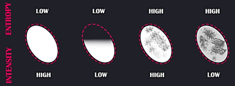
• Low Entropy, Low Intensity: The prediction is considered good. The eye may be in the half-closed position or even if the segmentation result is of low probability, it may still better compared to the alternatives.

• Low Entropy, High Intensity: The prediction is considered very well, and the eye is in the open position.

• High Entropy, Low Intensity: The prediction is deemed very poor.

• High Entropy, High Intensity: The prediction is considered good, and the eye is open, but it can be said that there are various obstacles or reflections on the pupil.

image010.png

Figure 5. The visualization of Entropy and Intensity concepts

(Pupil regions in a segmentation map are shown with white color. Pink ellipses represent the fitted parameters using pupil regions)

The visual representation of the above inferences is provided in Figure 5. According to this figure, when the entropy metric is low to medium and intensity is high, it indicates successful segmentation. On the other hand, the segmentation map can vary depending on the subject's eye appearance and environmental conditions. Therefore, the entropy-intensity values that will distinguish segmentation as successful and unsuccessful will also be specific to each experimental session. To dynamically determine this range and differentiate a successful segmentation, a formula is used based on the last 120 entropy and intensity values (or those within the about last 1 second, to be defined according to the system frequency) with newly calculated values. The comparison simply attempts to detect anomalies in entropy and intensity by using variance. In this way, entropy anomalies that suddenly rise too much or intensity anomalies that suddenly falls too much can be detected. Accordingly, the pupil ellipse is considered successful if ${{M}_{Ent}}>\max \left( {{L}_{Ent}} \right)+var\left( {{L}_{Ent}} \right)$ and ${{M}_{Int}}<\min \left( {{L}_{Int}} \right)+var\left( {{L}_{Int}} \right)$and unsuccessful if it is false. ${{L}_{Ent}}~$and ${{L}_{Int}}~$refer to last 120 data points for entropy and intensity metrics, respectively.

In the PETA correction step, the last successful ellipse parameter is used instead of the pupil ellipse marked as unsuccessful. However, a condition has been set for this use, and any ellipse parameters that do not meet this condition are not corrected with the previous successful one. The relevant condition is that the difference between the unsuccessful ellipse center point and the last successful ellipse center point is greater than 19 pixels. The threshold value of 19 pixels is the upper band value obtained according to the preparation procedures of the LPW dataset [81]. The threshold value is grounded in the following assumptions and reasoning:

(i) Eyeball Area Within Camera Detection: It is assumed that the area of the eyeball can fit within the area that the eye camera can detect. For example, if the image collected by the eye camera is 320×240 pixels, the eyeball is expressed with roughly 240×240 pixels.

(ii) Maximum Angular Velocity of the Human Eye: A human eye can have a maximum angular velocity of 700 degrees per second [82]. Since this is a peak value allowed to only 25 degrees of visual angle, we decreased it as maximum 500 degrees for LPW dataset [83].

(iii) Frame Rate of LPW Dataset: LPW dataset is 120 Hz. Therefore, the maximum angular velocity that a human eye can achieve between two frames is 4,166 degrees (500/120). 

(iv) Upper Coordinate Distance: In a 2D image, the largest difference in pixel coordinates resulting from a change in eyeball angle between two frames occurs when the geometry forms an isosceles triangle, as illustrated in Figure 6. Consequently, we computed a maximum shift of 8,723 pixels for an angular change of 4,166 degrees.

(v) Upper Band Threshold Values: Upon identifying that the maximum distance between two center points differed by approximately 9 pixels, we applied the widely accepted 5-pixel margin of error as per the literature for each center point. When we account for this 10-pixel permissible error difference (adding 5 pixels to each center point), the value utilized in our study was became 19 pixels for the upper bound. The relevant equalization rounded to nearest can be seen in the below. ${{\omega }_{max}}$, ${{f}_{cam}}$, ${{r}_{eye}},~E\left[ \varepsilon  \right]~$parameters denote 500, 120, 120, 5 values, respectively.

$Th{{r}_{upp}}=\sqrt{2{{r}_{eye}}^{2}\left( 1-\cos \left( \frac{{{\omega }_{max}}}{{{f}_{cam}}} \right) \right)}+2E\left[ \varepsilon  \right]+0.5$                  (13)

The upper band threshold value, denoted as $Th{{r}_{upp}}~$provide a solution to the problem of jumping data, especially during blinking or in cases where insufficient pupil information occurs due to any obstacle. However, the value of 19 pixels is not applied to pupil ellipse parameters that are marked as successfully/normal according to entropy and intensity values. In this way, if it is assumed that the segmentation is fulfilled successfully according to the metrics, the difference between the calculated and annotated pupil ellipses is prevented in cases such as the movement of the eye camera or the displacement of the pupil center point when the eye is reopened.

tu_pian_1.png

Figure 6. PETA upper bound threshold value representation between two consecutive center points for LPW dataset. The value is about 9 pixels, however we defined it as 19 pixels together with 5-pixel errors

The analysis of the present traditional method for LPW dataset are given in Table 2 with details. The table presents average measurements in terms of patch size, contained pupil area (CPA) and success. Patch size is the ratio of the generated patch resolution to the original image resolution. Contained pupil area indicates the percentage of the pupil is present in the generated patch. In this analysis, we assume that the ellipse can be fitted if at least 40% of the pupil area is in the patch. Success is obtained according to this assumption. A patch was considered successful if it contained at least 40% of the pupil area and unsuccessful otherwise. 

Consequently, the success value represents the ratio of successful detections to the total number of detections. To show the maximum positive effects of the traditional method, the PFX, PFY, and THM functions used were selected manually. For this, all sessions were analyzed with each function combination and the functions that would give the best performance were selected by the authors. Basically, the following equalization has been calculated for all combinations and configurations, with the highest score has been selected for each different LPW session. Also in the auto configuration mechanism, the same regime was processed to find traditional configurations for the segmentation map generated using full image received every once in a certain period.

 $Score=\left( 100-Patch~Size \right)*CPA$                       (14)

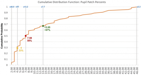
On average, the patch resolution was 7.66 times smaller (13.05% of original resolution) than the original image resolution, containing 95.51% of the total pupil area, and achieving a patch generation success rate of 99.23%. However, in the next analyses, we will use the average patch size as 6×, not 7.66×, for ease of calculation. In addition, the Cumulative Distribution Function (CDF) curve of the average pupil patch percentages calculated on a video basis is given in Figure 8.

Accordingly, although the average patch percentage value is 13.05% and the average magnification factor is 7.66×, within the scope of the CDF, half of the videos have been reduced to a percentage of 7.58% or smaller. Thus, for half of the videos, the magnification factor is equal to or greater than 13.2×. On the other hand, the probability related to the intuitive 20% pupil size applied when determining the window size of the Savitzky-Golay filter is also shown in the graph. According to this, a 20% window size on each axis results in a patch that is 4% of the total image. Accordingly, in 23% of the images analyzed within the scope of LPW, a patch size of 4% or smaller, and thus a magnification factor of 25× or larger, has been achieved. The maximum and minimum magnification factors obtained within the scope of LPW are 46.9× and 2.2×, respectively. However, the accumulation in the distribution generally occurs at patch sizes of 2% and 8%, where the graph accelerates rapidly.

Table 2. The results of the traditional method according to parameters selected manually for each session of LPW

The examination of the selected learning models within the scope of the study is presented in Table 3. Generally, the models produced similar dice scores for the LPW-3Hz dataset. The source of this similarity is that the LPW dataset contains pupil information that can be well detected by a learning model. On the other hand, small differences in scores distinguish the models from each other. This difference arises from cases that are relatively less common in the LPW dataset. Examples of such cases include blinking, strong reflections, and a large angle of the gaze vector relative to the eye camera. Therefore, small improvements in scores indicate that the model is more robust in inadequate pupil information. Hence, UNet++, UNet++-S, TransUNet, and TransUNet-S models are the best-performing models in terms of both dice and test dice scores. Therefore, it can be said that any of these four models can be used for pupil detection.

Another goal of this study is to aim for a real-time (at 120 Hz and above) and less resource-consuming system. GPU performances in terms of inference time and memory requirements for both original resolution (320×240px) and the resolution of the average patch size (107×120px). According to the measurements, UNet-S, UNet++-S, SegNet-VGG-S and CCSGD-RN-34-S perform shortest inference time, while UNet-S, SegNet-VGG-S, TransUNet-S, all PPMobileSeg models, and EGEUnet require less resource area.

The learning model part of the study will be run in GPU. However, investigating models on only CPU may put an insight off related to sufficiency of models for devices with less capacity such as mobile phones. CPU analysis includes similar measurements like the GPU analysis. The relevant performance metrics are shown in Table 3. Accordingly, CCSGD-RN-34, CCSGD-RN-34-S, EGEUNet and all PPMobileSeg models perform fairly successfully results while compared to others.

In the stage of the learning model phase of the ROM concept, the UNet++-S model was selected after reviewing the relevant analyses. This selection was made because the UNet++-S model has produced successful Dice scores and stands out in terms of resource requirements. This model can operate in approximately 6 milliseconds on a GPU using pupil patches and requires 340 MB of space, achieving 95.6% success in training and 86% in testing. Consequently, the UNet++-S model has been used in all other analyses as the   learning model. However, it can be said that the CCSGD-RN-34-S model is more prominent in CPU usage due to the balance between speed and performance.

Table 4 provides training sessions of the UNet++-S model with different LPW variations and their corresponding test measurements. According to this, there is a significant correlation between the resolution in the training set and the test dice score of UNet++-S. In general, as the difference between the resolution in the training set and the test input resolution increased, the dice score decreased. On the other hand, LPW-AV has been able to produce successful results in all variations since it was trained with all training variations. Additionally, training UNet++-S with all variations (LPW-AV) has also increased the test dice score of each variation except x6. The inability to significantly increase the x6 test dice score may be related to the fact that the training with LPW-AV was limited to 15 epochs. However, this situation was not considered, and the UNet++-S model trained with LPW-AV was used in the continuation of the study. 

Table 3. Inference time, consumed memory, and dice metrics for selected learning models trained with 3Hz LPW

image015.png

Figure 8. Cumulative distribution function for average pupil patch percent of the traditional method

Table 4. UNet++-S model training with different variations of the LPW dataset to display the effect of the input size to the accuracy

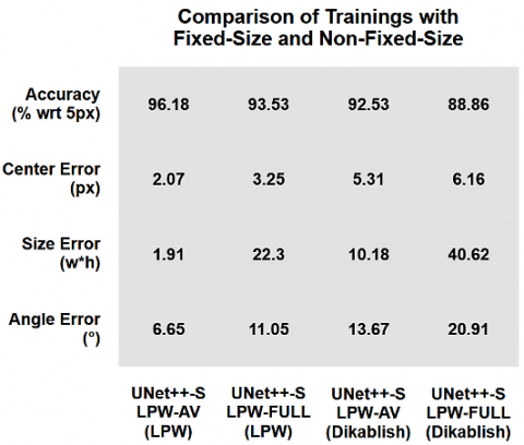
In the next analysis, the impact of the study components on accuracy was assessed, and relevant measurements are presented in Table 5. While L and D refer to LPW and Dikablis datasets, LM and TM refer to the learning model and traditional method, respectively. AUTO denotes the automatic traditional method configuration mechanism. In addition, measurements were made for two alternatives of AUTO that run every 100ms and 333ms. The results were calculated based on a 5-pixel error and average ellipse parameter error. Ellipse error consists of pixel errors in center point (x, y), size (major, minor) and angle error, respectively. During the analysis, it was seen that the traditional method's patch area may not be at a sufficient level for the learning model and ellipse fitting operations. Therefore, the patch taken from the traditional model was analyzed by expanding it to 20px from the bottom and left, and 10px from the top and right edges for LPW. If an edge does not have enough space to be expanded, the corresponding edge is expanded to the maximum possible space. As a result of LPW analyses, the extended traditional model patch has a resolution of 19.50% compared to the original image, corresponding to an average resolution of ×5 for the learning model. For Dikablis, average patch size was 10.27% and CPA amount was 94.60%, by using traditional configurations in accordance with scores of each combination. In measurements made with LPW for the average patch size to be similar, the patch area was expanded by 30 pixels from the bottom and 22 pixels from the left in the vertical direction. Therefore, the results were approximately taken as having ×5 resolution for Dikablis as well. Furthermore, since the Dikablis dataset’s preparation frequency of 25 Hz, the upper band value was set at 52 pixels for the Dikablis, according to the calculation explained in Eq. (13).

Also, in the analysis of the LPW and Dikablis datasets, three procedures were applied. Firstly, no binarization operation was applied to the segmentation maps when the results were obtained. In other words, the maps obtained from the model were used directly for the analysis. Secondly, the model trained with LPW-AV was used in all analyses, including ones without traditional method. Normally, one might consider using the model trained with LPW-Full for the analyses without the traditional method because LPW-AV was generated for models predicting in accordance with different input resolutions. However, as shown in Figure 9, we discovered that LPW-AV has a data augmentation effect. Training the model with different resolutions, even though it operates at a fixed resolution, results in a significant improvement in accuracy. In the figure, four performance metrics are shown. Accuracy represents successful detections based on a 5-px error value. Center error is the average error between the estimated and annotated ellipse center coordinates. Size error is presented as the product of the average errors in width and height between the estimated and annotated ellipses. Angle error represents the average angular errors between the estimated and annotated ellipses. Lastly, if the width or height values of the ellipse parameters calculated in Dikablis are smaller than 5 pixels, the previously calculated ellipse was used. With the use of the 5-px size regime, the UNet++-S trained with LPW-AV achieved an accuracy rate of 92.53%, while in the case where it was not used, the accuracy rate was 92.47%. Although the success difference is quite low, a size-dependent adjustment in models trained with different resolutions, such as LPW-AV, may have the potential to increase success to a certain extent.

Table 5. Accuracy metrics for the combination of the study components

image016.png

Figure 9. Comparison of models trained with LPW-Full and LPW-AV. Accordingly, LPW-AV, containing different resolution of same images

Table 6. Average GPU pred. times of UNet++-S for input resolutions at different subsampling rates in millisec

Consequently, according to Table 5, over 92% was achieved for both LPW and Dikablis datasets. In a situation where traditional model configurations were determined manually, only a 1% 5-px loss of accuracy was observed compared to a flow where only the learning model was used, for LPW dataset. Furthermore, it is observed that the automatic configuration mechanism has relatively little impact on accuracy. The patch size obtained is the same as the patch rate obtained from AUTO, but the success rate obtained from AUTO may be 2.5% lower.  Especially, the fact that success does not significantly decrease with the use of this mechanism was crucial for the usability of this mechanism. Thereby this situation may reduce the need for the user to adjust on the traditional method.

Table 6 presents the prediction time of the UNet++-S model at different resolutions. Specifically, the selected model exhibits runtimes of 25.41 milliseconds at full resolution, 5.57 milliseconds with the average patch size (×6), and 6.12 milliseconds with the extended average patch size (×5).

Table 7. Average GPU execution times of the study sub-components except for the learning model in millisec

image017.png

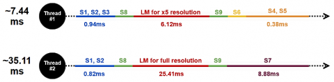
Figure 10. Execution times of the pipeline working with two threads for detection and auto configuration processes

Table 8. Worst case in performance changes of auto-configuration mechanism and its comparison with ROM and ROM-PETA model

Table 7 displays the GPU execution times for various subcomponents used in the study. Apart from these, the running time of some mathematical operations and control expressions that will require less computing power has been ignored. Figure 10 provides a graphical representation of the execution times for the proposed pipeline on the GPU. Notably, the pupil detection process requires approximately 7.5 milliseconds, while the auto-configuration mechanism, which operates on a separate thread, requires 35 milliseconds. Consequently, it can be inferred that pupil detection can be performed at a rate exceeding 120 Hz.

Table 8 presents the worst-case runtimes of the auto-configuration mechanism under two variants: ROM-only (R) and ROM combined with PETA (RP). As noted in Table 7, the automatic selection of traditional method parameters typically completes within 8.88 ms. Since this selection process occurs on the CPU while segmentation is executed on the GPU, parallelism ensures that the auto-configuration mechanism introduces minimal latency to the overall detection process. However, when auto-configuration is not executed during the segmentation but only after segmentation and by processing only a few parts of the selection in each frame, its frequency affects inference time and FPS. For example, an AUTO-10Hz setting implies one selection operation every 100 ms, whereas AUTO-3Hz corresponds to a 333 ms interval. Under this scheduling, auto-configuration introduces an average latency of approximately 0.9 ms per frame at 10 Hz and about 0.1 ms at 3 Hz. Moreover, the less frequently traditional parameters are recalculated, the more the performance tends to degrade. As shown in the table for the Dikablis dataset, reducing the auto-configuration frequency from 10 Hz to 3 Hz results in roughly a 1% drop in accuracy. Nonetheless, using the 10 Hz variant leads to only a modest decrease in core performance, approximately 0.40% - which may be considered an acceptable trade-off for maintaining high responsiveness.

ping_mu_jie_tu_2025-08-13_150535.png

Dikablis (a subset of TEyeD) is larger (320, 200 images), collected from a different eye tracker, and more challenging regarding illumination. Hence, training on LPW was validated with Dikablis. The recent and popular OpenEDS dataset was developed for eye tracking in VR systems. Although suitable for evaluating the proposed method's performance in VR [84], OpenEDS was not included since our amplitude-based approach would require additional procedures to avoid pupil searches in dark regions caused by VR headsets. Based on this, we haven’t analyzed VR images in the current scope of the study [96, 97].

When determining dataset variations for LPW, image resolutions were not set uniformly but were instead prepared in accordance with the CDF curve and the intuitively defined 4% pupil size information. Accordingly, variations start from the lowest magnification factor of ×2 and end at the intuitive value related to the average pupil size, which is ×25, as given in the CDF graph. Intermediate resolution variations are not created at equal intervals but are instead based on regions of accumulation in the CDF. Therefore, variations with resolutions of ×25, ×16, ×9, and ×6 are prepared for areas with high accumulation. Those with resolutions of ×4, ×2, and the original are referenced for areas with less accumulation. However, for a more comprehensive solution, resolution variations can be diversified, and more frequent resolution choices can be made even in areas with less accumulation.

Unlike edge-based methods and learning models, amplitude-based traditional methods in the literature can enable the implementation of pre-experimental precautions to enhance computational accuracy. These precautions are generally associated with the removal of regions darker than the pupil from the eye area. However, this may not always be possible, and there may be dark areas in the eye region that cannot be removed. Therefore, in such cases, it should not be expected that traditional methods using amplitude information will work accurately. The amplitude-based traditional method proposed in the ROM concept of this study does not operate on the assumption that the pupil is the darkest region. Instead, it allows the experimental operator to determine the relationship between the pupil and other dark areas and operates according to PF function selections. PF functions provide a pre-experimental precaution alternative that is more advantageous than other amplitude-based traditional methods by evaluating the darkness, length, and position information of the pupil simultaneously. On the other hand, the First and End function, which ensures the selection of all dark areas, can be used to maximize the likelihood of the pupil being included within the patch, even in extreme situations where pre-experimental precautions cannot be taken. In this regard, the proposed amplitude-based traditional method can inspire measures regarding pupil selection criteria in other methods that operate with traditional processes.

While training and comparing the learning models in the study, certain regulations were implemented to reduce the training duration on the fixed hyperparameters and the data set. For a more accurate analysis, training processes can be designed with the all the data set (not with 3 Hz set), cross-validation and hyperparameter optimizations. However, due to our temporal and physical resources, the relevant regulation had to be implemented. Also, the proposed model was tested at 320×240 resolution, commonly used in eye tracking. Evaluating its performance at different resolutions is important for robustness, and we consider this a direction for future work. On the other hand, training the proposed UNet++-S entirely on an unseen dataset (non-IR and structurally different from pupil data) is considered future work, as it would further strengthen the model’s claims of generalizability.

In the literature, pupil detection successes are often reported using metrics such as center error and accuracy based on a 5-pixel error. These metrics may be inadequate for comparing models, as the mean value is insufficient to define a stochastic process producing ellipse parameters. Therefore, the comparison section includes not only performance metrics based on ellipse center points but also size and angle errors. Sharing these metrics in future studies might better reflect the performance that studies can offer. On the other hand, sharing size and angle errors is crucial for understanding the success of a segmentation model working with pupil patches. This is because, in cases where the patches created are small-sized and well-centered by the pupil, the success of the segmentation model may not be apparent. To better understand the performance of the segmentation model, average size error and the average size of the created patches can serve as good indicators.

With the operation of the ROM concept, a learning model with a traditional method can operate more efficiently with less unnecessary information. This is especially prominent in the field of remote eye tracking, as direct pupil information cannot be obtained by capturing the entire scene. Many objects in the scene may be black or circular, like the pupil. Therefore, in remote eye tracking, facial detection is first performed, and the eye region is then extracted, and lastly pupil is segmented. In other words, in remote eye trackers, several procedures are applied to ensure that learning models receive only the most relevant information. This study demonstrates that the "most relevant visual information" principle, which remote eye tracking systems already apply, can also be additionally implemented for wearable eye tracking systems.

In deep learning studies, training sets may be given to training after being cropped. However, in this type of cropping, the resolution of the cropped image is rescaled towards the fixed resolution in the dataset. Although a similar cropping approach has been applied in LPW-AV, resolutions have not been expanded to the original resolution. Additionally, LPW-AV, which includes cropped images at different resolutions, has a data augmentation effect and has been able to significantly improve performance. On the other hand, within the scope of this study, it has not been investigated whether this increase in success is due to different resolutions or only cropping. Furthermore, while exploring the impact of these two cropping approaches on pupil detection could be a different research topic, almost none of the studies in the literature have fixed-size cropping been used as a data augmentation method.

Models designed to work with pupil patches were trained with LPW-AV, which combines all LPW variations. However, this increases the training duration cost. For example, while one epoch UNet with LPW-Full is completed in approximately 3-4 hours, LPW-AV takes about 10-12 hours for one epoch. To reduce this cost during training, two regimes can be applied. The first is to select a certain number of samples from each LPW variation rather than using all variations, creating a new mixed LPW variation. The second is to complete this process with synthetic image generators. The working principle of a synthetic image generator could be to produce images at a lower resolution, where the model makes less successful predictions in real-time. We do not explore these two alternatives within the concept of reducing training times and attribute this research as future work. On the other hand, in the ROM structure, if a model is used whose success is not affected by the input resolution, there is no issue with a variation like LPW-AV and, consequently, no problem of increased training time.

The existing literature has highlighted the utilization of various eye features for diverse applications, emphasizing the potential value of exploring new features. However, our model is designed to find pupil ellipse parameters only. Making the developed model detectable for other eye features can be considered as another future work of this study.

Parameters marked as unsuccessfully according to PETA's metrics are not corrected if they do not meet the condition in the correction approach. It may be considered to improve the current correction approach to correct the unsuccessful parameters mentioned, but our study aimed to provide a solution for serious jumping data only. In addition, PETA's upper band recommendation is only for the human eye. For the developed method to be used in an animal other than a human, the assumptions will need to be updated according to the relevant animal.

The threshold of 19 pixels, as determined in PETA's upper band correction approach, is notably high, and its impact on improving performance is minute. For a more optimal upper band, the eyeball can be detected, and then the angular change between two consecutive frames can be observed. However, since our method does not detect eyeballs in its current form, it had to offer a procedure that produces higher upper band values. The integration of an eyeball detection feature or method has the potential to further enhance the accuracy of the PETA correction. However, on the other hand, this correction method with or without eyeball parameters may be useful for traditional pupil detectors. When the model is also capable of detecting the eyeball, steps 1 and 4 in Section 2.3 — which include the empirical procedures for calculating the PETA threshold — will no longer be necessary. Consequently, it becomes possible to directly apply a function like the one in Equation 13 to the desired eye tracker without relying on prior assumptions. However, integrating an eyeball detection mechanism and adapting the function to determine the upper-bound threshold based on the detected eyeball region are considered as the next steps of this study.

ROM runs at an average of 6.5 ms per frame on GPU—approximately 4× faster than UNet and UNet++-S, and 6× faster than UNet++. This corresponds to 153 FPS for ROM, compared to 35, 39, and 25 FPS for UNet, UNet++-S, and UNet++, respectively. On CPU, ROM achieves around 17 FPS, while the others drop to 1.5–2.5 FPS. While we expect similar speed advantages on such systems, measuring inference time on low-resource hardware is planned as future work to better assess ROM's scalability. ROM also requires significantly less RAM (~340 MB vs. ~1700 MB for UNet) and is compatible with compression techniques like quantization and pruning. Further acceleration is possible with TensorRT or ONNX, especially on lower-end devices.

ROM represents an approach rather than a rigid structure, allowing flexibility in the models and methods employed. According to the naming used in this study, works that combine traditional methods with learning models are referred to as ROM studies. Consequently, ROM presents an opportunity for future research, enabling researchers in the pupil detection field to explore innovative studies based on the fusion of traditional and state-of-the-art techniques. Additionally, from this perspective, we attribute LEyes' pupil detector as a study within the ROM concept.

As mentioned in the literature review, the most recent pupil detection studies are [42, 43, 50, 52, 58-63]. In our comparison with PONet, the proposed model not only performs more accurately due to its lack of limitation to 15 positions but also generates pupil area information thanks to its segmentation feature [61]. This is a crucial feature for cognitive studies. While EV-Eye provides a high-level frequency, it is more expensive, non-wearable, and likely less accurate. Therefore, pupil detection frame by frame with CMOS cameras remains a necessity. Res-CNN achieves a significant portion of its frequency increase by reducing resolution [63]. However, as resolution decreases, the error rate increases. Our proposed ROM structure, on the other hand, crops the image instead of reducing the resolution. Although the QAT structure in Res-CNN is not used in our study, it can be adapted. This would provide an additional frequency increase. Furthermore, the SAM-based model, Vir-NET, and Mal-NET can be directly expressed with the ROM structure [43, 50, 52]. Thus, it is possible to develop new studies that improve the detection speeds of all three models. A similar observation can be made for Byrne et al. [58]. For more accurate results, incorporating noise reduction and segmentation map correction operations into ROM, along with improving learning model accuracy, can be a function to be tested in future studies. However, Jamaludin et al.’s studies work according to black amplitude and lack the accuracy of a learning model. As mentioned in the literature, black amplitude information can easily produce erroneous results due to its insufficiency. On the other hand, the ROM structure is not valid for Pistol [39]. This is because Pistol focuses on detecting multiple components that can spread across the entire image, requiring the model input to be evaluated as a whole. However, as stated in the study, if a single segmentation model is used to improve performance, it is possible to add the Pistol model to the learning model part of ROM solely for pupil and iris detection. PCR-Net is also unsuitable for ROM for a similar reason as Pistol, as it focuses on detecting non-pupil eye components for remote systems [42].