Jeyalakshmi Gangadharan![]() | Shahul Hameed Kopuli Ashkar Ali*
| Shahul Hameed Kopuli Ashkar Ali*![]()
© 2025 The authors. This article is published by IIETA and is licensed under the CC BY 4.0 license (http://creativecommons.org/licenses/by/4.0/).
OPEN ACCESS
Nowadays, Brain tumours are the most crucial disease that is spreading rapidly all around the world. According to the statistics, more than a thousand people are losing their lives to this tumour in every country. The early prediction of tumours can help to diagnose and overcome the disease quickly. For an earlier prediction, there are Numerous research techniques like deep learning (DL) and machine learning (ML) models used for feature extraction and classification. In some cases, the hybrid models are also used for feature extraction and classification. However, the accuracy is not attained up to the level of satisfaction for various tumours like Glioma, pituitary, and meningioma. We propose a novel DenseNet architecture incorporating Self-Calibrated Squeeze-and-Excitation (SC-SE) for enhanced feature extraction and representation. The SC-SE DenseNet integrates SC Convolutions (SC-Conv) and SE Blocks within a DenseNet framework. SC-Conv dynamically recalibrates both spatial and channel-wise features, which improves the model’s ability to adapt to diverse input variations. SE blocks are used to concentrate important channels for better feature learning. The extracted features from SC-SE DenseNet are classified using the XGBoost classifier. To further optimize performance, the Fire Hawk Optimizer (FHO) is used for feature selection and hyperparameter tuning. FHO aids in selecting the most relevant features from the input image and reduces dimensionality. Additionally, FHO is used to fine-tune the parameters of the XGBoost classifier to increase the classification accuracy.
feature extraction, DenseNet model, fire Hawks optimization, self-calibrated (SC)
The brain is the most important part of the human organ which comprises all the nervous system responsibilities of every activity. Based on the World Health Organization (WHO), Brain Tumour is the most severe disease of the human brain that have an irregular brain cell pattern. This tumour has several types, namely secondary and primary metastatic brain tumour [1]. The primary is a brain tumour that originates from human brain cells, which is a non-cancerous disease. But in secondary metastatic tumours, it spreads to other body parts, to the brain, through the blood.
Based on WHO, Brain Tumours is into four different categories, such as Grade I to Grade IV [2]. These Grades are categorised based on their malignant or benign. The malignant tumour can affect other parts of the human body. Also, benign tumour never attacks nearby tissue or other organs of the human body. To predict the brain tumour, magnetic resonance imaging (MRI) and computer tomography (CT) are used as standard methods so far. The malignant tumours, Grade III and Grade IV, are very aggressive brain tumours that also affect other parts.
In some cases, there are three major primary brain tumours, namely Glioma, pituitary and meningioma [3]. The glioma tumours develop from the brain’s glial cells. The Pituitary tumour is a type of benign tumor that develops in the pituitary gland. This gland provides a few essential hormones in the body and also forms a base layer of the brain. The Meningioma tumours develop in a protective membrane of the spinal cord and brain. These types of tumours can be diagnosed if it is predicted earlier. But unfortunately, the MRI and CT cannot provide that much accuracy in prediction.
In recent times, the medical field has emerged with a machine learning (ML) and deep learning (DL) models of its higher training rate. The ML and DL models are very supportive of earlier prediction by training huge datasets of tumour images [4]. Some of the popular DL and ML methods that are applied for medical applications are Convolutional Neural Networks (CNN), Support Vector Machine, AdaBoost, Naive Bayes, Decision Tree, DenseNet, GoogLeNet, VGGNet, ResNet, AlexNet, Recurrent Neural Network (RNN), and Long Short-Term Memory (LSTM), etc. These learnings are methods used for classification and feature extraction models for an early diagnosis.
In brain tumour classifications, the current approaches struggle to identify and use the most relevant features from medical images. Existing feature extraction techniques, such as traditional CNNs, may fail to capture complex patterns in MRI images due to their limited ability to model spatial dependencies and multi-scale features. Furthermore, feature selection methods in existing systems are often either too simplistic or computationally expensive. It leads to either a loss of crucial information or the inclusion of irrelevant features.
Nowadays, to enhance the prediction ability, metaheuristic methods are used as problem-solving models. These methods are inspired by and developed from the nature and biological behaviour of birds and animals. The metaheuristics methods are used to find the optimal solution among all possible solutions. The metaheuristics methods are applied to a medical application.
This work proposes a superior approach by combining SC-SE DenseNet for advanced feature extraction and FHO for optimized feature selection. This hybrid method not only improves the relevance and quality of the selected features but also enhances classification accuracy by curtailing the impact of redundant or noisy features. The remaining part of this work is contributed in the following: in Section 2, the related works based on brain Tumours are described. Section 3 discusses the proposed work. Section 4 discusses the experimental results, and the paper concludes with a conclusion and references.
In this section, the literature papers are described by various authors which is related to the brain tumour classification. Some of the recent methods with greater innovation are mentioned in this section.
Ezhov et al. [5] presented a learnable proxy to simulate the growth of a tumour. This growth is mapped to a biophysical model parameter, directly to simulation outputs. Whereas the patient geometry is obtained through local tumour cell densities and improves the accuracy of classification. In the literature, a 2-D CNN-based spectral-spatial HSI classification and feature extraction is presented by Hao et al. [6]. Also, the fusion and optimization model are done with edge-preserving filtering. Next, the DL models (AlexNet, GoogLeNet, ResNet101, ResNet50, and SqueezeNet) are presented for a malignant and benign classification. This model proved that the AlexNet accomplished higher accuracy than any other DL model, which is described by Mehrotra et al. [7].
Zhou et al. [8] developed brain tumour detection with missing modalities. This method used a correlation method to signify the hidden multi-source correlation among multi-modalities. These modalities are fused through an attention mechanism, which improves the performance of detection. Some work has applied a DL model with a handcrafted fusion and features that are proposed by Ramzan et al. [9]. This model applied a grab model and morphological operations with a DL model classification. These features are processed with various classifiers and achieve a higher accuracy.
The pre-trained GoogLeNet is used for tumour classification by Deepak et al. [10]. This DL model has attained a greater accuracy than the traditional methods of art methods. In literature, Çinar and Yildirim [11] developed a hybrid DL architecture to predict the Brain Tumour. The ResNet50 model is used in it, which has added 8 layers to the CNN instead of the last 5 layers. This hybrid model achieved a higher maximum accuracy than a conventional ResNet50 model. Next, the Deep Neural Network (DNN) is used to categorize the MRI-based brain tumour by Mohsen et al. [12]. Here, a fuzzy c-means clustering model is used to split a normal and abnormal MRI. The feature extraction is done by the discrete wavelet transform (DWT).
Yu et al. [13] presented a sample-adaptive intensity lookup table (LuT) for MRI-based brain tumours. This method transformed the intensity contrast of every input dynamically to adapt to it. The SA-LuT-Nets results showed superior performance with single and multiple MR modalities. Next, the lightweight deep model known as the One-pass Multi-task Network (OM-Net) is used for brain tumour detection by Zhou et al. [14]. It resolved a class imbalance and correlated among several tasks. It has both an online training data transfer method and a curriculum learning method.
Singh et al. [15] proposed an ensemble model combining ResNet50 and EfficientNet-B7 for brain tumour classification with an accuracy of 95.68%. Zhang et al. [16] introduced a deep residual network optimized by an enhanced Heap-based Optimization (HO) algorithm. The optimized residual model achieves 96.64% accuracy in medical image classification. Nag et al.'s [17] TumorGANet, using ResNet50 and Generative Adversarial Networks (GAN) achieved 95% accuracy. Nassar et al. [18] used a multi-model system with an accuracy of 99.31%. Talukder et al. [19] applied transfer learning with ResNet50V2. It shows 94.68% accuracy for the public MRI dataset. Salve and Jondhale [20] developed a Hybrid Deep Convolutional Neural Network with the Deer Hunting (Hybrid DCNN-DH) method for tumor grade classification. Patil and Kirange [21] introduced an Ensemble Deep Convolutional Neural Network (EDCNN) model, which achieved 96.67% accuracy.
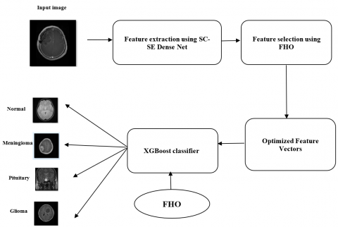
The proposed system outlines a method for efficient brain tumor categorization using MRI images. The steps involved in the proposed system are given in Figure 1. Initially, feature extraction is performed using SC-SE DenseNet. It is used to capture detailed characteristics from the MRI images. Then, feature selection is applied to increase the relevant features while eliminating redundant ones. The optimized feature vectors are fed into the XGBoost classifier for robust classification. Finally, FHO is used again to fine-tune the feature set and optimize the classification model’s performance.
Figure 1. Proposed workflow
3.1 SC-SE DenseNet
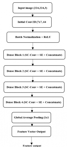
The SC-SE DenseNet is a modified version of DenseNet that integrates Self-Calibrated Convolutions (SC-Conv) and Squeeze-and-Excitation (SE) Blocks to improve the feature extraction and representation. The SC-SE DenseNet consists of an initial convolutional layer, four densely connected blocks (Dense Blocks), and a global average pooling (GAP) layer to extract more relevant features of the input image. The architecture of SC-SE DenseNet is given in Figure 2.
Figure 2. Proposed SC-SE DenseNet architecture
3.1.1 SC-Conv
The SC-Conv improves feature extraction by dynamically calibrating the input features based on their spatial and contextual information. This is achieved through the combination of two parallel paths: the Standard Convolution Path and Self-Calibration Path. The Standard Convolution Path extracts spatial features using conventional convolution operations. The Self-Calibration Path dynamically adjusts feature representations using global context information. Let the input feature map be $\mathrm{X} \in \cdot \mathbb{R}^{H \times W \times C}$, where H denotes the height of the feature map, W denotes the width of the feature map and C denotes the number of channels. The SC-Conv operation is defined as:
$Y=F_{ {conv }}(X)+F_{ {calibrate }}(X)$ (1)
where, $Y=F_{ {conv }}(X)$ is the output of the standard convolution path and $Y=F_{ {calibrate}}(X)$ is the output of the self-calibration path. This Standard Convolution Path applies a conventional convolution operation. It can be defined as;
$F_{{conv}}(X)=W * X+b$ (2)
where, * denotes the Convolution operator, W denotes the weights of the convolutional kernel and b is the bias term. The self-calibration path involves three key steps: Global Context Extraction, Channel-Wise Calibration and Feature Recalibration. For global context extraction, it computes a spatial summary of X using global average pooling as follows:
$g_c=\frac{1}{H \times W} \sum_{h=1}^H \sum_{w=1}^W X(h, w, c)$ (3)
where, $g_c$ represents the aggregated information for channel c. The result $\mathrm{g} \in \mathbb{R}^C$ Captures the global context. For channel-wise calibration, the global context vector g is calibrated through a learnable transformation:
$s=\sigma\left(W_s g\right)$ (4)
where, $W_s$ is the learnable weight matrix, σ is the non-linear activation function, $\mathrm{g} \in \mathbb{R}^C$ is the calibrated scaling vector for each channel. For feature recalibration, the calibrated vector s is used to reweight the original input as follows:
$F_{ {calibrate }}(X)=X \odot s$ (5)
where, ⊙ denotes element-wise multiplication. The final output Y of the SC-Conv operation integrates both paths:
$Y=F_{ {conv }}(X)+F_{ {calibrate }}(X)$ (6)
3.1.2 SE
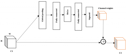
The SE block is a powerful mechanism in neural networks designed to enhance the representational power of CNNs [22]. This block is inserted to concentrate on important features and suppress the irrelevant features. The SE block works by learning channel-wise feature recalibration weights and allowing the network to adaptively attend to essential features. This process involves two fundamental operations: squeezing and exciting as shown in Figure 3. The squeezing step aggregates channel-wise information to capture global statistics and the exciting step performs feature re-weighting based on learned parameters.
Figure 3. SE block
In Squeeze operation, it compresses the spatial dimensions of X into a channel descriptor by performing global average pooling. In an excitation operation, the squeezed vector passes through a fully connected (FC) bottleneck network with two layers to capture channel dependencies. Overall, the SE block focuses purely on recalibrating the channel importance of feature maps using global context. The SC-Conv improves feature extraction by combining spatial and channel recalibration. It includes both standard convolutions and a dynamic self-calibration path.
3.2 Fire Hawk Optimizer (FHO)
The metaheuristic model [23] of the FHO method is inspired by the hunting strategy of black kites, whistling kites, and brown falcons that are known as Fire Hawks. These birds are often used to set a fire around the prey to catch them [24].
Initially, the fire hawk is positioned as the prey in its territory. The fire hawk is considered to catch in its territory and protect that not affected by other fire hawks. The distance limit between the number of the prey and the fire hawk is estimated. Meanwhile, position updation is performed by fire hawks so that the prey from its territory is not affected by other territories' fire hawks. The Gaussian distribution is used to provide a search loop in random where the number of prey and total fire hawks are estimated.
Core Principles of FHO:
(1) Initialization
A population of potential solutions (denoted X) is initialized randomly within the bounds of the problem's search space. Each solution vector represents a candidate position in the d-dimensional problem space. It can be mathematically defined as:
$x_j^i(0)=x_{j, \text { min }}^i+r_1\left(x_{j, \text { max }}^i-x_{j, \text { min }}^i\right)$ (7)
where, $x_{j, \min }^i$ and $x_{j, \max }^i$ are the bounds, $r_1$ is a uniform random number, i=1,2,…,N, and j=1,2,…,d.
(2) Classification into Fire Hawks and Prey
In this stage, the candidates with better objective function values become fire hawks and others represent prey. Fire hawks spread "fires" strategically to herd prey into more favourable search regions. The total distance between each fire hawk and its nearest prey is computed to define territories as follows:
$D_l^k=\sqrt{\left(x_2-x_1\right)^2+\left(y_2-y_1\right)^2}$ (8)
This calculation ensures each fire hawk's territory is distinguished for optimal search coverage.
(3) Position Updates
Fire Hawks (FH) adjust their positions based on proximity to the global best solution (GB) and influence from other hawks. It can be mathematically defined as:
$F H_l^{{new }}=F H_l+r_1\left(G B-F H_l\right)-r_2\left(F H_{ {near }}-F H_l\right)$ (9)
where, $r_1$ and $r_2$ are random coefficients, l is the index for FH. l=1,2,…,n. n is the total number of fire hawks in the search space. Likewise, the prey reacts by moving within or outside fire hawk territories.
$P R_q^{\text {new }}=P R_q+r_3\left(F H_l-P R_q\right)-r_4\left(S P_l-P R_q\right)$ (10)
where, $S P_l$ represents a safe zone or position within the fire hawk’s territory, q is the index of Prey Reactions (PR).
(4) Iterative Search and Optimization
Fire hawks simulate dynamic behaviors like dropping burning sticks and expanding their territories, while prey constantly adapts to escape threats. These steps refine solution quality iteratively.
3.3 FHO-based feature optimizations
Feature selection is an essential step of DL models which identifies the most relevant input features and eliminates irrelevant or redundant ones. In this work, feature selection is combined into the DenseNet model using the FHO to improve the tumor classification accuracy. For feature optimization, the FHO is initialized with a population of candidate solutions. Each candidate denotes a subset of the features extracted by the proposed DenseNet. The population is randomly set, where each solution relates to a different combination of features.
The pseudocode for the proposed feature selection is given below:
|
Start: Input: Dataset D (features F and labels Y), population size N, max iterations MaxIter Initialize population (N solutions) with random positions (feature subsets) Evaluate the fitness of each solution using classification error (XGBoost) While not MaxIter: # Exploration Phase (Fire Hawks vs Prey) For each candidate solution i in population: Classify solutions into Fire Hawks and Prey based on fitness: - Fire Hawks are solutions with better fitness - Prey represent the remaining solutions Identify better-performing solutions (Fire Hawks) Select a random solution SPi from Prey (Safe Position for Prey) Fire Hawks spread "fires" to herd Prey into better regions of the feature space # Update position of Prey based on Fire Hawks’ influence: Update Prey position: $P R_q^{{new }}$ # Exploitation Phase (Position Updates for Fire Hawks) For each Fire Hawk l in population: Update position based on proximity to the global best solution (Xbest): $FH_l^{ {new }}$ If the new position improves fitness (lower classification error): Replace the current feature subset with updated subset. # Update global best solution Xbest if a better fitness is found: If Fitness (Xi) > Fitness (Xbest): X_best = Xi End While Output: Best feature subset (Xbest) and its corresponding Classification error. |
Each solution is calculated using a fitness function that measures the classification loss of a classifier trained on the selected features. The algorithm refines the feature subsets by identifying better-performing solutions (Fire Hawks) and selecting random solutions from this set. The current feature subset is updated based on these better solutions. The solution is accepted when the update improves the classifier’s performance. The process continues until convergence, with the algorithm returning the best feature subset corresponding to the minimum classification error. This subset represents the most relevant features for the classification task.
3.4 FHO-based parameter tuning
XGBoost is a robust ensemble learning method used for classification tasks [25]. The performance of the XGBoost model is greatly influenced by the hyperparameters. It includes the learning rate, maximum tree depth, and the number of estimators. The proper tuning of these hyperparameters improves the model’s accuracy and efficiency. In this work, FHO is used to identify the optimal hyperparameter configuration for XGBoost. This technique accelerates the optimization process and increases the overall model performance. The pseudocode for the proposed parameter tuning is given below:
|
Pseudocode: FHO for XGBoost Hyperparameter Tuning Start: Input: Dataset D (features F, labels Y), Population Size N, Max Iterations MaxIter Initial Range for XGBoost Hyperparameters (learningrate, maxdepth, nestimators, etc.) Number of generations MaxGenerations Initialize Population with random hyperparameter values within the defined range: Each solution is represented by a vector Xi = [learningrate, maxdepth, nestimators, ...] For each candidate solution i in the Population, evaluate fitness: Fit XGBoost model with hyperparameters Xi and calculate Classification error. Fitness (Xi) = Model Accuracy While not MaxGenerations: # Exploration Phase (Fire Hawks vs Prey) For each candidate solution i in Population: Classify solutions into Fire Hawks and Prey based on fitness: - Fire Hawks have better objective function values - Prey represent the rest of the population Identify better-performing solutions (Fire Hawks) and select a random solution SPi from Prey (Safe Position for Prey). Fire Hawks spread "fires" strategically to herd prey into more favorable regions. # Update position of Prey based on Fire Hawks’ influence: Update Prey position: $P R_q^{ {new }}=P R_q+r_3\left(F H_l-P R_q\right)-r_4\left(S P_l-P R_q\right)$ # Exploitation Phase (Position Updates for Fire Hawks): For each Fire Hawk l in Population: Update position based on proximity to the global best solution (Xbest): $F H_l^{ {new }}=F H_l+r_1\left(G B-F H_l\right)-r_2\left(F H_{{near }}-F H_l\right)$ If new position improves fitness: Replace current hyperparameters with updated ones. # Update global best solution Xbest if a better fitness is found: If Fitness (Xi) > Fitness (Xbest): Xbest = Xi End While Output: Best Hyperparameters (Xbest) for XGBoost Corresponding Evaluation Metric (Classification error) End |
The population is initialized randomly. The solutions are classified based on their fitness values whereas Fire Hawks represent better solutions. Fire Hawks adjust their positions based on proximity to the global best solution (Xbest) and prey. The prey reacts to the influence of Fire Hawks. The fitness of each solution guides the optimization process in both the exploration and exploitation phases.
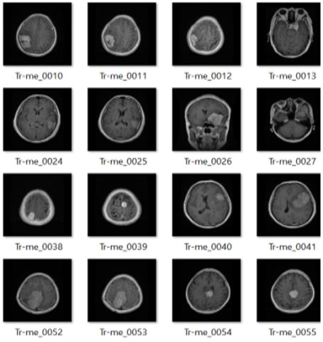
The dataset used for this work was obtained from the Kaggle websitehttps://www.kaggle.com/datasets/masoudnickparvar/brain-tumor-mri-dataset). The images are provided in .jpg format to standardize input values; all images are resized to 224 × 224 pixels, and pixel intensities are normalized to the range [0, 1] by dividing by 255. The dataset included 490 Glioma Tumors, 364 Meningioma Tumors, 617 Pituitary Tumors, and 423 No-tumour images. The dataset is divided into a 70% training set and a 30% test set. The test set contained 147 Glioma Tumors, 109 Meningioma Tumors, 185 Pituitary Tumors, and 127 No-tumour images. The visualization of data set images is shown in Figure 4.
Figure 4. Dataset visualization
The program is written using Python (IDLE 3.7) with TensorFlow 3.10 and accelerated by NVIDIA CUDA 11.2. Here, metrics like Sensitivity, Accuracy, F1 Score, and Precision are attained for evaluation. These metrics are derived from the confusion matrix that includes True Negatives (TN), True Positives (TP), False Negatives (FN), and False Positives (FP). Then, the performance metrics can be computed as follows:
Accuracy $=\frac{\mathrm{TP}+\mathrm{TN}}{\left(\mathrm{TP}+\mathrm{TN}+\mathrm{FP}+\mathrm{FN}^{\prime}\right)}$ (11)
Recall $=\frac{\mathrm{TP}}{\left(\mathrm{TP}+\mathrm{FN}^{\prime}\right)}$ (12)
Precision $=\frac{\mathrm{TP}}{\left(\mathrm{TP}+\mathrm{FP}^{\prime}\right)}$ (13)
F 1 score $=2 \cdot \frac{\text { Precision } \cdot \text { Recall }}{\text { (Precision }+ \text { Recall })}$ (14)
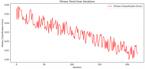
The feature optimization process using FHO is given in Figure 5. For optimization, the fitness function is framed as a function of classification error. Over the iterations, the fitness value shows a decreasing error value, which indicates an improvement in feature selection. Initially, the fitness varies significantly as the optimizer explores the feature space. As iterations increase, the algorithm converges toward lower classification errors. It is observed that the FHO is able to refine the feature set effectively and reduce computational overhead without compromising accuracy.
Figure 5. Feature selection fitness curve
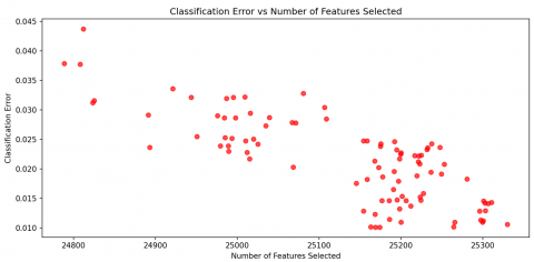
Figure 6. Feature optimization curve
The relationship between the number of features selected and the corresponding classification error is given in Figure 6. It shows that reducing the number of features generally leads to lower classification errors. This focuses on the effectiveness of the FHO in choosing a high-quality feature set for the classification task. Before optimization, the model's computational complexity is higher with a feature size of 50,233. After optimization, the feature size was significantly reduced to 24,019 with lower memory requirements.
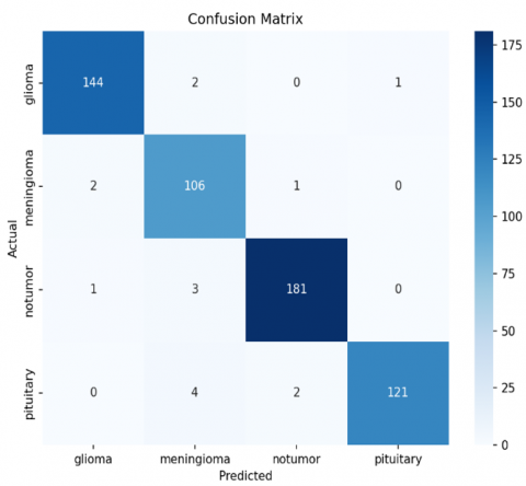
(a) With FHO
(b) Without FHO
Figure 7. Confusion matrix analysis
Figure 7 shows the confusion matrix analysis of the SC-SE DenseNet model. The proposed model with FHO is better in terms of accuracy, precision, recall, and F1 score compared to those without FHO. This suggests that the FHO optimization technique has increased the model's performance in classifying tumor stages.
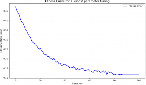
Figure 8. Fitness curve for XGBoost parameter tuning
Figure 8 shows the fitness curve for XGBoost parameter tuning as a function of classification error. The curve shows a sharp decline in the initial iterations, which indicates that the model is learning rapidly at the start. The final classification error stabilizes at approximately 0.10, which denotes a relatively low error achieved with the tuned parameters. The optimal values for the XGBoost model parameters are presented in Table 1. Specifically, the optimal learning rate is 0.4, the maximum depth is 5, the optimal number of estimators is 154, and the gamma value is 2.5.
Table 1. Parameter analysis
|
Hyperparameter |
Lower Bound |
Upper Bound |
Optimized Value |
|
Learning Rate |
0.01 |
0.5 |
0.4 |
|
Max Depth |
3 |
15 |
8 |
|
Number of Estimators |
50 |
200 |
154 |
|
Gamma |
0 |
5 |
2.5 |
To ensure the reproducibility of hyperparameter tuning, we fixed the random seed to 42 during all FHO runs and conducted five repeated trials. The metric variance across multiple runs for the SC-SE DenseNet+FHO model is given in Table 2. The model shows a high mean accuracy of 97.40% with a small standard deviation (± 0.36%), which denotes stable performance across runs. Additionally, the F1-Score and AUC-ROC values of 98.2 and 0.970, respectively. It proves the model's strong ability to balance precision and recall rates.
Table 2. Metric variance analysis of the model
|
Metric |
Mean (±Std) SC-SE DenseNet+FHO |
|
Accuracy |
97.40% ± 0.36% |
|
F1-Score |
98.2 ± 0.011 |
|
AUC-ROC |
0.970 ± 0.006 |
Table 3. Ablation study of the model
|
Metric |
Without SC-Conv (SE + FHO) |
Without SE Block (SC-Conv + FHO) |
Without FHO (SC-Conv + SE) |
Proposed SC-SE DenseNet + FHO |
|
Precision |
97.45 |
97.10 |
98.30 |
99.43 |
|
Recall |
97.10 |
96.80 |
97.20 |
98.59 |
|
F1-Score |
97.25 |
96.90 |
97.80 |
99.0 |
|
Accuracy |
97.55 |
97.10 |
97.80 |
98.94 |
|
AUC-ROC |
0.98 |
0.97 |
0.98 |
0.987 |
The performance of the models with the component impact is given in Table 3. The proposed model with FHO achieved the greatest accuracy, precision, recall, and F-Score rates of 98.94%, 99.43%, 98.59%, and 99%, respectively. It proves the model's ability to classify tumor stages correctly with balanced performance. The model without SC-Conv shows slightly reduced performance, which indicates the importance of feature learning. Additionally, the absence of the SE block leads to a further decrease, which highlights the importance of the SE block in feature recalibration. Similarly, the proposed model without FHO achieved the lowest accuracy, precision, recall, and F-Score rates of 97.8%, 98.3%, 97.20%, and 97.8%, respectively. The performance comparison with other models is given in Table 4. Other models, such as the EDCNN Model, Vision Transformer, and TumorGANet, show moderate performance with accuracies of 96.7%, 97.80% and 97.4%, respectively. These models failed to match the robustness and adaptability of the SC-SE DenseNet model. Overall, the integration of FHO into the proposed DenseNet not only enhances its classification accuracy but also increases its precision, recall, and F1-score rates.
Table 4. Performance comparison with other models
|
Model |
Accuracy (%) |
Precision (%) |
Recall (%) |
F1-Score |
AUC-ROC |
|
AlexNet |
88.40 |
87.9 |
87.3 |
87.5 |
0.910 |
|
Transfer Learning (ResNet50V2) |
94.80 |
94.6 |
94.5 |
94.6 |
0.962 |
|
Hybrid ResNet50 + EfficientNet-B7 |
95.68 |
95.3 |
95.5 |
95.4 |
0.965 |
|
TumorGANet |
97.40 |
97.5 |
97.2 |
97.3 |
0.978 |
|
Hybrid DCNN-DH |
94.00 |
93.8 |
93.5 |
93.6 |
0.950 |
|
DL with HO |
96.70 |
96.4 |
96.2 |
96.3 |
0.971 |
|
GoogleNet |
93.45 |
92.7 |
93.1 |
93.0 |
0.944 |
|
SqueezeNet |
94.60 |
94.2 |
94.0 |
94.1 |
0.955 |
|
EDCNN Model |
96.70 |
96.2 |
96.5 |
96.4 |
0.969 |
|
Vision Transformer (ViT-B/16) [26] |
97.80 |
97.3 |
97.1 |
97.2 |
0.985 |
|
Swin Transformer [27] |
98.1 |
97.9 |
97.7 |
97.8 |
0.987 |
|
Proposed SC-SE DenseNet + FHO |
98.90 |
98.7 |
98.6 |
98.7 |
0.991 |
Table 5. Performance comparison of FHO with other optimizers
|
Optimizer |
Accuracy (%) |
Convergence Speed (Iterations) |
Training Time (Seconds) |
|
FHO |
98.9 |
50 |
15 |
|
Grey Wolf Optimizer (GWO) [28] |
97.2 |
85 |
22 |
|
Particle Swarm Optimization (PSO) [29] |
95.6 |
120 |
30 |
|
GA (Genetic Algorithm) [30] |
94.8 |
150 |
45 |
The comparison of FHO with other standard optimization algorithms is given in Table 5. The FHO optimizer shows the highest accuracy with the fastest convergence speed and the shortest training time. In contrast, GWO and PSO show slightly lower accuracy, but GWO achieves faster convergence than PSO.
Table 6. Performance comparison of XGBoost with other classifiers
|
Classifier |
Accuracy (%) |
Precision |
Recall |
F1-Score |
|
Proposed Model (XGBoost) |
98.9 |
99.43 |
98.6 |
0.99 |
|
SVM (Support Vector Machine) [31] |
96.5 |
95.2 |
94.8 |
0.945 |
|
Random Forest [32] |
97.2 |
96.5 |
96.1 |
0.960 |
|
Logistic Regression [33] |
94.1 |
92.8 |
92.5 |
0.925 |
|
K-Nearest Neighbors (KNN) [34] |
95.8 |
94.2 |
93.9 |
0.939 |
The performance comparison of the XGBoost model with other classifier models is given in Table 6. The proposed XGBoost model outperforms other classifiers with the highest accuracy of 98.9% due to the boosting mechanism in XGBoost, which sequentially improves weak learners to reduce errors effectively. The other classifiers failed to perform iterative error correction processes.
Statistical significance analysis
To validate the superiority of the proposed SC-SE DenseNet model with FHO, a statistical significance analysis is conducted using multiple evaluation metrics. The results of the experiments were repeated over five independent runs to calculate the average values and standard deviations of the key metrics: accuracy, precision, recall, and F1-score. Table 7 gives the averages and variances for the proposed model compared to baseline models, including EDCNN, TumorGANet, and the model without FHO optimization.
Table 7. Statistical significance analysis
|
Metric |
Model |
Mean (%) |
Standard Deviation (%) |
|
Accuracy |
SC-SE DenseNet with FHO |
98.94 |
0.12 |
|
|
SC-SE DenseNet without FHO |
97.53 |
0.18 |
|
|
TumorGANet |
97.40 |
0.20 |
|
Precision |
SC-SE DenseNet with FHO |
99.43 |
0.10 |
|
|
SC-SE DenseNet without FHO |
96.92 |
0.15 |
|
|
TumorGANet |
97.02 |
0.18 |
|
Recall |
SC-SE DenseNet with FHO |
98.59 |
0.14 |
|
|
SC-SE DenseNet without FHO |
97.08 |
0.19 |
|
|
TumorGANet |
97.25 |
0.22 |
|
F1-Score |
SC-SE DenseNet with FHO |
99.00 |
0.11 |
|
|
SC-SE DenseNet without FHO |
96.97 |
0.16 |
|
|
TumorGANet |
97.13 |
0.19 |
Table 8. Paired t-test results
|
Metric |
Comparison |
p-value |
Statistical Significance |
|
Accuracy |
SC-SE DenseNet with FHO vs. TumorGANet |
0.001 |
Yes |
|
|
SC-SE DenseNet with FHO vs. EDCNN |
0.0008 |
Yes |
|
Precision |
SC-SE DenseNet with FHO vs. TumorGANet |
0.002 |
Yes |
|
Recall |
SC-SE DenseNet with FHO vs. TumorGANet |
0.003 |
Yes |
|
F1-Score |
SC-SE DenseNet with FHO vs. TumorGANet |
0.0015 |
Yes |
|
AUC-ROC |
SC-SE DenseNet with FHO vs. TumorGANet |
0.004 |
Yes |
|
Specificity |
SC-SE DenseNet with FHO vs. TumorGANet |
0.002 |
Yes |
To further ensure the statistical robustness of the results, paired t-tests are conducted between the proposed model and the competing models. The tests were performed at a 95% confidence level (significance threshold of α = 0.05) to determine whether the observed improvements were statistically significant. The p-values obtained for the comparison of accuracy, precision, recall, F1-score, Area Under the Curve- Receiver Operating Characteristic (AUC-ROC), and specificity are summarized in Table 8.
The results confirm that the proposed model significantly outperforms competing models in all metrics. The low standard deviations indicate consistent performance across multiple runs, and the p-values validate that the improvements are statistically significant. To further improve the statistical analysis, we have applied multiple-testing corrections like the Bonferroni correction. This method adjusts the significance threshold to account for the increased risk of Type I errors (false positives) when multiple tests are conducted. For example, given that multiple comparisons are made between the SC-SE DenseNet with FHO and TumorGANet, the Bonferroni correction was applied to adjust the p-value threshold for each test. It is used to observe whether the differences in performance are statistically significant and not due to chance. The p-values accurately reflect the significance of the observed differences and reduce the risk of Type I errors due to multiple comparisons.
The computational analysis of the proposed model is given in Table 9. The integration of FHO slightly increases training time, but the inference speed remains within acceptable clinical limits and proves the suitability for real-time implementation. Compared to the Vision Transformer, SC-SE DenseNet shows faster inference with reduced memory usage.
Table 9. Computational analysis of the proposed model
|
Model |
Training Time (hrs) |
Inference Time (ms/image) |
GPU Used |
|
SC-SE DenseNet |
2.3 |
12 |
NVIDIA RTX 3090 |
|
SC-SE DenseNet+FHO |
3.1 |
15 |
NVIDIA RTX 3090 |
|
Vision Transformer |
4.2 |
20 |
NVIDIA RTX 3090 |
Table 10. Performance of the model with other data sets
|
Dataset |
Accuracy (%) |
Precision (%) |
Recall (%) |
F1-score |
|
Kaggle |
98.94 |
99.43 |
98.59 |
0.99 |
|
BraTS |
97.85 |
97.6 |
97.3 |
0.974 |
|
TCIA |
96.92 |
96.5 |
96.1 |
0.964 |
To address the practical challenges and ethical considerations mentioned, the proposed model was further validated using an additional publicly available dataset of BraTS [35] and TCIA [36]. This cross-dataset evaluation is used for reliable results across different clinical settings and patient demographics. The obtained results are given in Table 10. In the BraTS dataset, the proposed model achieves an accuracy, precision, recall, and F1-score of 97.85%, 97.6%, 97.3%, and 0.974, respectively. Similarly, on the TCIA dataset, it achieves 96.92% accuracy, 96.5% precision, 96.1% recall, and an F1-score of 0.964. This proves the model's robustness for integration into hospital workflows with its adaptability across real-world data variations.
In conclusion, the proposed feature optimization framework effectively addresses the limitations of brain tumor classification in MRI images. The use of DenseNet for feature extraction confirms that complex image patterns are captured. It focuses on the relevant features and reduces redundant computational complexity. Additionally, FHO is used for choosing discriminative features and fine-tuning hyperparameters. It increases the model's accuracy and classification performance. Future research should address the practical challenges by integrating explainable AI with hospital workflows through cloud-based solutions.
[1] de Robles, P., Fiest, K.M., Frolkis, A.D., Pringsheim, T., Atta, C., St. Germaine-Smith, C., Day, L., Lam, D., Jette, N. (2015). The worldwide incidence and prevalence of primary brain tumors: A systematic review and meta-analysis. Neuro-Oncology, 17(6): 776-783. https://doi.org/10.1093/neuonc/nou283
[2] Tamimi, A.F., Tamimi, I., Abdelaziz, M., Saleh, Q., Obeidat, F., Al-Husseini, M., Haddadin, W., Tamimi, F. (2015). Epidemiology of malignant and non-malignant primary brain tumors in Jordan. Neuroepidemiology, 45(2): 100-108. https://doi.org/10.1159/000438926
[3] Saba, T., Rehman, A., Altameem, A., Uddin, M. (2014). Annotated comparisons of proposed preprocessing techniques for script recognition. Neural Computing and Applications, 25: 1337-1347. https://doi.org/10.1007/s00521-014-1618-9
[4] Siegel, R.L., Miller, K.D., Jemal, A. (2018). Cancer statistics, 2018. CA: A Cancer Journal for Clinicians, 68(1): 7-30. https://doi.org/10.3322/caac.21442
[5] Ezhov, I., Mot, T., Shit, S., Lipkova, J., Paetzold, J.C., Kofler, F., Pellegrini, C., Kollovieh, M., Navarro, F., Li, H., Metz, M., Wiestler, B., Menze, B. (2022). Geometry-aware neural solver for fast Bayesian calibration of brain tumor models. IEEE Transactions on Medical Imaging, 41(5): 1269-1278. https://doi.org/10.1109/TMI.2021.3136582
[6] Hao, Q., Pei, Y., Zhou, R., Sun, B., Sun, J., Li, S., Kang, X. (2021). Fusing multiple deep models for in vivo human brain hyperspectral image classification to identify glioblastoma tumor. IEEE Transactions on Instrumentation and Measurement, 70: 1-14. https://doi.org/10.1109/TIM.2021.3117634
[7] Mehrotra, R., Ansari, M.A., Agrawal, R., Anand, R.S. (2020). A transfer learning approach for AI-based classification of brain tumors. Machine Learning with Applications, 2: 100003. https://doi.org/10.1016/j.mlwa.2020.100003
[8] Zhou, T., Canu, S., Vera, P., Ruan, S. (2021). Latent correlation representation learning for brain tumor segmentation with missing MRI modalities. IEEE Transactions on Image Processing, 30: 4263-4274. https://doi.org/10.1109/TIP.2021.3070752
[9] Ramzan, F., Khan, M.U.G., Rehmat, A., Iqbal, S., Saba, T., Rehman, A., Mehmood, Z. (2020). A deep learning approach for automated diagnosis and multi-class classification of Alzheimer's disease stages using resting-state fMRI and residual neural networks. Journal of Medical Systems, 44: 37. https://doi.org/10.1007/s10916-019-1475-2
[10] Deepak, S., Ameer, P.M. (2019). Brain tumors classification using in-depth CNN features via transfer learning. Computers in Biology and Medicine, 111: 103345.
[11] Çinar, A., Yildirim, M. (2020). Detection of tumors on brain MRI images using the hybrid convolutional neural network architecture. Medical Hypotheses, 139: 109684. https://doi.org/10.1016/j.mehy.2020.109684
[12] Mohsen, H., El-Dahshan, E.S., El-Horbaty, E.S., Salem, A.B. (2018). Classification using deep learning neural networks for brain tumors. Future Computing and Informatics Journal, 3(1): 68-71. https://doi.org/10.1016/j.fcij.2017.12.001
[13] Yu, B., Zhou, L., Wang, L., Yang, W., Yang, M., Bourgeat, P., Fripp, J. (2021). SA-LuT-Nets: Learning sample-adaptive intensity lookup tables for brain tumor segmentation. IEEE Transactions on Medical Imaging, 40(5): 1417-1427. https://doi.org/10.1109/TMI.2021.3056678
[14] Zhou, C., Ding, C., Wang, X., Lu, Z., Tao, D. (2020). One-pass multi-task networks with cross-task guided attention for brain tumor segmentation. IEEE Transactions on Image Processing, 29: 4516-4529. https://doi.org/10.1109/TIP.2020.2973510
[15] Singh, R., Gupta, S., Bharany, S., Almogren, A., Altameem, A., Rehman, A.U. (2024). Ensemble deep learning models for enhanced brain tumor classification by leveraging ResNet50 and EfficientNet-B7 on high-resolution MRI images. IEEE Access, 12: 178623-178641. https://doi.org/10.1109/ACCESS.2024.3494232
[16] Zhang, L., Qiao, Z., Li, L. (2024). An evolutionary deep learning method based on improved heap-based optimization for medical image classification and diagnosis. IEEE Access, 12: 102745-102773. https://doi.org/10.1109/ACCESS.2024.3433483
[17] Nag, A., Mondal, H., Hassan, M.M., Al-Shehari, T., Kadrie, M., Al-Razgan, M., Alfakih, T., Biswas, S., Bairagi, A.K. (2024). TumorGANet: A transfer learning and generative adversarial network-based data augmentation model for brain tumor classification. IEEE Access, 12: 103060-103081. https://doi.org/10.1109/ACCESS.2024.3429633
[18] Nassar, S.E., Yasser, I., Amer, H.M., Mohamed, M.A. (2024). A robust MRI-based brain tumor classification via a hybrid deep learning technique. Journal of Supercomputing, 80(2): 2403-2427. https://doi.org/10.1007/s11227-023-05549-w
[19] Talukder, M.A., Islam, M.M., Uddin, M.A., Akhter, A., Pramanik, M.A.J., Aryal, S., Almoyad, M.A.A., Hasan, K.F., Moni, M.A. (2023). An efficient deep learning model to categorize brain tumor using reconstruction and fine-tuning. Expert Systems with Applications, 230: 120534. https://doi.org/10.1016/j.eswa.2023.120534
[20] Salve, A.K., Jondhale, K.C. (2023). An improved grade based MRI brain tumor classification using hybrid DCNN-DH framework. Biomedical Signal Processing and Control, 85: 104973. https://doi.org/10.1016/j.bspc.2023.104973
[21] Patil, S., Kirange, D. (2023). Ensemble of deep learning models for brain tumor detection. Procedia Computer Science, 218: 2468-2479. https://doi.org/10.1016/j.procs.2023.01.222
[22] Hu, J., Shen, L., Sun, G. (2018). Squeeze-and-excitation networks. In Proceedings of the IEEE Conference on Computer Vision and Pattern Recognition, pp. 7132-7141.
[23] Kavitha, V.P., Sakthivel, B., Deivasigamani, S., Jayaram, K., Ahmad, R.B., Keita, I.S. (2024). An efficient modified black widow optimized node localization in wireless sensor network. IETE Journal of Research, 70(12): 8404-8413. https://doi.org/10.1080/03772063.2024.2384486
[24] Azizi, M., Talatahari, S., Gandomi, A.H. (2022). Fire Hawk Optimizer: A novel metaheuristic algorithm. Artificial Intelligence Review, 56: 287-363. https://doi.org/10.1007/s10462-022-10173-w
[25] Divya, K.S., Bhargavi, P., Jyothi, S. (2020). XGBoost classifier to extract asset mapping features. Advances in Computational and Bio-Engineering, 15: 195-208. https://doi.org/10.1007/978-3-030-46939-9_18
[26] Chen, X., Liu, C., Hu, P., Lin, J., Gong, Y., Chen, Y., Peng, D., Geng, X. (2024). Adaptive masked autoencoder transformer for image classification. Applied Soft Computing, 164: 111958. https://doi.org/10.1016/j.asoc.2024.111958
[27] Wu, X., Feng, Y., Xu, H., Lin, Z., Chen, T., Li, S., Qiu, S., Liu, Q., Ma, Y., Zhang, S. (2023). CTransCNN: Combining transformer and CNN in multilabel medical image classification. Knowledge-Based Systems, 281: 111030. https://doi.org/10.1016/j.knosys.2023.111030
[28] Mirjalili, S., Mirjalili, S.M., Lewis, A. (2014). Grey wolf optimizer. Advances in Engineering Software, 69: 46-61. https://doi.org/10.1016/j.advengsoft.2013.12.007
[29] Kennedy, J., Eberhart, R. (1995). Particle swarm optimization. In Proceedings of ICNN'95-International Conference on Neural Networks, Perth, Australia, pp. 1942-1948. https://doi.org/10.1109/ICNN.1995.488968
[30] Alhijawi, B., Awajan, A. (2024). Genetic algorithms: Theory, genetic operators, solutions, and applications. Evolutionary Intelligence, 17: 1245-1256. https://doi.org/10.1007/s12065-023-00822-6
[31] Chaganti, S.Y., Nanda, I., Pandi, K.R., Prudhvith, T.G.N.R.S.N., Kumar, N. (2020). Image classification using SVM and CNN. In 2020 International Conference on Computer Science, Engineering and Applications, Gunupur, India, pp. 1-5. https://doi.org/10.1109/ICCSEA49143.2020.9132851
[32] Xu, B., Ye, Y., Nie, L. (2012). An improved random forest classifier for image classification. In 2012 IEEE International Conference on Information and Automation, Shenyang, China, pp. 795-800. https://doi.org/10.1109/ICInfA.2012.6246927
[33] Song, Z., Wang, L., Xu, X., Zhao, W. (2023). Doubly robust logistic regression for image classification. Applied Mathematical Modelling, 123: 430-446. https://doi.org/10.1016/j.apm.2023.06.039
[34] Nakata, K., Ng, Y., Miyashita, D., Maki, A., Lin, YC., Deguchi, J. (2022). Revisiting a KNN-based image classification system with high-capacity storage. In European Conference on Computer Vision, pp. 1-16. https://doi.org/10.1007/978-3-031-19836-6_26
[35] Wei, C., Ren, S., Guo, K., Hu, H., Liang, J. (2024). Dataset: BraTS 2021. https://doi.org/10.57702/tgzceeph
[36] Liu, X., Shih, H.A., Xing, F., Santarnecchi, E., El Fakhri, G., Woo, J. (2024). Dataset: TCIA. https://doi.org/10.57702/9oevh8zk