T. Jemima Jebaseeli![]() | Anandakumar Haldorai
| Anandakumar Haldorai![]() | Hye Jin Kim*
| Hye Jin Kim*![]()
© 2025 The authors. This article is published by IIETA and is licensed under the CC BY 4.0 license (http://creativecommons.org/licenses/by/4.0/).
OPEN ACCESS
Purtscher Retinopathy (PR) is a severe vision-threatening disorder that is frequently connected with trauma, severe pancreatitis, or connective tissue diseases. Conventional diagnostic techniques depend on fluorescein angiography and clinical examination, both of which can be intrusive and may not always yield conclusive results. Spectral-Domain Optical Coherence Tomography (SD-OCT) is a non-invasive imaging technique that produces high-resolution cross-sectional images of the retina and allows for accurate evaluation of retinal layers and illnesses. The proposed method implements a panoptic segmentation algorithm to detect PR using SD-OCT image data in an unsupervised manner. The Panoptic Feature Pyramid Network (FPN) detects and categorizes clinical indications of PR using instance and semantic segmentation. To detect additional challenging factors, a deep Convolutional Neural Network (CNN) is combined with encoder-decoder structures and instance segmentation networks. When it came to recognizing and classifying retinal disorders connected to PR, the proposed approach showed excellent accuracy. The performance of the proposed method was assessed using quantitative measures such as the Intersection over Union (IoU), Dice coefficient, pixel accuracy, precision, recall, and F1 score. This approach offers a non-invasive and efficient tool for the early detection of PR, allowing for timely management and better patient outcomes.
Purtscher Retinopathy (PR), OCT, spectral-domain OCT, panoptic segmentation, Panoptic Feature Pyramid Network (FPN)
The most common imaging method for eye disease diagnosis is OCT. Faster acquisition and optical penetration depth are two advantages of Spectral-Domain Optical Coherence Tomography (SD-OCT) for retinal imaging [1]. It demonstrates how hyper-reflective the retinal layers are. The considerable rendering of the long wavelength SD-OCT makes it superior to the short wavelength SD-OCT. TD-OCT, or Time Domain-OCT, is the initial version of OCT. FD-OCT, or Fourier Domain-OCT, is the name of the second-generation OCT. SS-OCT (Swept Source-OCT) is the next generation of OCT after FD-OCT [2]. SD-OCT offers less signal decay and a longer wavelength of depth images to produce deeper penetration of observation. It gives relevant differences among individual retinal layers by its contrast to highlight the clinical variations. OCT provides a valuable assessment of Purtscher Retinopathy’s (PR) condition [3]. When typical retinal signs are present without evidence of trauma, the condition is known as Purtscher-Like Retinopathy (PLR) [4]. PR was invented in 1910 by Otmar Purtscher [5]. He found a man who had fallen from a tree with head damage. It occurs mainly due to head and thorax traumas. PR can also be caused by chest compression, femur fractures, long bone fractures, crush traumas to bones, avulsion fractures, humeral tuberosity, shoulder joint dislocation, and barotrauma.
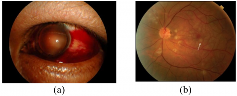
PR is used to represent the retinopathy occurrence in the eyes due to trauma, acute pancreatitis, FES (Fat Embolism Syndrome), childbirth, and renal failure. There will be 0.24 cases per million population rise in the PR year [6]. As shown in Figure 1, the disease is marked by cotton wool patches, intra-retinal haemorrhages, and flecks. Leukoembolization, endothelial damage, C5, and blockade of arterioles are the implications of PR.
Figure 1. Pathological PR: (a) Sub-conjunctival hemorrhage, (b) Purtscher Flecken is highlighted in the arrow [7]
The occlusion causes Purtscher Flecken on the capillary bed. The nerve fiber layer infarcts and leads to retinal whitening spots of different sizes. This is the reason for bilateral vision loss among the patients. Purtscher Flecken refers to the many polygonal intra-retinal whitening patches located at the posterior pole and surrounding the optic disk [7].
The infection of the outer retina is difficult to visualize due to the thick layers that occur in the acute phase. The photoreceptors also get affected at this phase.
Microperimetry gives the functional side of morphological alterations on OCT [8]. Increased thoracic pressure causes venous reflex and leads to endothelial damage. There might be 50 microns on either side of the retinal arterioles and venules. In rare cases, whiteness surrounds the venules. It is possible that a pseudo-cherry-red patch is present in the macula. The lesions along the nerve fiber layer on the retinal surface may be elevated by the white cotton wool patches. At that point, the lesions' border will become indistinct. Further causes subsequent occlusion due to microvascular circulation incompetence.
The novelty of the proposed approach combines advanced imaging and segmentation techniques to provide an accurate, non-invasive diagnostic tool for PR, with the potential for improving clinical practices and patient care.
The proposed system offers the following novel contributions.
The proposed approach introduces a unique unsupervised panoptic segmentation framework for identifying PR from SD-OCT images, overcoming the limitations of previous diagnostic tools.
Unlike conventional methods that depend on fluorescein angiography and manual clinical assessment, which are invasive and subjective, the proposed approach utilizes high-resolution SD-OCT imaging for automated and non-invasive detection. Traditional deep learning-based segmentation models primarily utilize semantic segmentation, whereas this method employs a Panoptic FPN to integrate both semantic segmentation for pixel-wise classification of retinal abnormalities and instance segmentation for distinct identification of pathological elements such as cotton-wool spots and hemorrhages enabling precise lesion localization.
Unlike supervised deep learning models, which require extensive labeled datasets, this approach operates in an unsupervised manner, significantly reducing annotation dependency and enhancing applicability to rare diseases. The model architecture integrates a deep CNN-based encoder-decoder structure, optimizing multi-scale feature extraction for enhanced segmentation accuracy. The instance segmentation component is trained to separate overlapping pathological features, improving granularity in PR lesion detection. Additionally, multi-level feature fusion within the FPN ensures a robust hierarchical representation of PR-related clinical signs.
The article is structured in the following manner. Section 2 explains the literature review, Section 3 describes the dataset used in the study, Section 4 presents the proposed technique, Section 5 describes the research implementation, Section 6 describes the results and discussions, and Section 7 concludes the research.
Purtscher's and Purtscher-like retinopathy have an estimated yearly occurrence of 0.24 cases/million, and its identification is mostly symptomatic in the absence of a defined etiology [9]. Although the pathogenesis of Purtscher-like retinopathy is unknown, numerous ideas have been offered based on the fundamental systemic condition, although it is assumed to be induced by embolization that causes arteriolar blockage and ischemia [10]. The lesions indicate the existence of the disease, but they appear in only half of the patients. Individuals must be recognized from cotton-wool patches, which partially cover vessels and lack appropriate boundaries. PR patients frequently describe sudden, painless vision loss 2 to 48 hours after the underlying illness. Findings are frequently apparent bilaterally also be seen unilaterally [11-13].
Xiao et al. [14] developed multimodal imaging in PR, which revealed capillary nonperfusion, quantified the foveal avascular zone, and found an ellipsoid zone abnormality in acute PR. Optic disc enlargement, retinal edema, and pseudo-cherry spots may also appear in the early stages, yet they are less prevalent. In the majority of circumstances, the illness is bilateral [15, 16]. Four young women experienced severe bilateral sight loss due to numerous retinal arteriolar occlusions within 24 hours of delivery [17]. Preeclampsia complicated labor in two cases, necessitating a cesarean surgery. Rothbächer et al. [18] provided insight into PR after ENT surgery. The study lacks advanced imaging techniques like OCT angiography or fluorescein angiography that could have offered more detailed visualization of the retinal vasculature. These factors reduce the strength of the conclusions and highlight the need for further investigation.
Ophthalmoscopy and fluorescein angiography revealed signs of Purtscher's Retinopathy-like ischemia retinal whitening in several superficial peripapillary and macular regions. The white spots in the eyes of all four patients had disappeared after eight weeks, and three of them had much better visual acuity. The pathogenesis of this illness is unknown. It may include arteriolar blockage caused by complement-induced leukoemboli generated after parturition [19, 20].
The datasets for the proposed study are taken from 1980 to 2010 and come from Medline, EMBASE, ISI, EBSCO, Science Direct, and Google Scholar. Purtscher-like Retinopathy was identified in 10 of the 5688 individuals studied, in that, 9 are women and a man. Purtscher-like Retinopathy was found in 0.16% of people. With a range of 10 to 40 years, the average age was 25. The follow-up period lasted an average of 12 months. Ninety-three percent of patients had cotton wool patches, sixty-five percent had retinal hemorrhages, and sixty-three percent had Purtscher Flecken. The detailed description is shown in Table 1.
Table 1. The dataset used for experimentation
|
Total Individuals Studied |
5688 |
|
Purtscher-like Retinopathy Cases |
10 cases |
|
Gender Distribution |
Women: 9, Men: 1 |
|
Age Range |
10 to 40 years |
|
Average Age |
25 years |
|
Follow-up Duration |
Average: 12 months |
|
Lesion Types |
93% of patients with Cotton Wool Spots |
|
65% with Retinal Hemorrhages |
|
|
63% with Purtscher Flecken |
|
|
Total Number of Images |
10 PR images (from the 10 cases) |
|
Dataset Size (Training) |
70% of total images (7 images) |
|
Dataset Size (Validation) |
15% of total images (1 image) |
|
Dataset Size (Testing) |
15% of total images (2 images) |
PR is a painless visual activity problem and causes visual disturbance. To optimize the Panoptic FPN for detecting PR from SD-OCT images, several key modifications has been made to suit the specific characteristics and challenges of this medical imaging task. These changes primarily focused on the network’s architecture, preprocessing techniques, and fine-tuning of hyperparameters.
Figure 2 shows the structure of the proposed technique. Instance and semantic segmentation outputs are concurrently predicted by the proposed CNN. ResNet-50 serves as the foundation of the proposed network and was selected due to its capacity to extract reliable features from intricate medical images, including SD-OCT scans. By addressing the vanishing gradient issue, ResNet-50's residual connections make deep network training more effective. ResNet-50 balances model performance and computational efficiency in comparison to other possible backbones like ResNet-101 or EfficientNet. ResNet-101 has a deeper architecture that may be able to capture finer-grained information, but because of its greater complexity, training durations, and processing costs may rise. However, EfficientNet needs a lot of fine-tuning for medical image applications, even though it could provide better accuracy. ResNet-50 was selected due to its shown efficacy in medical imaging applications and its ability to handle large image datasets with manageable processing requirements.
Figure 2. Architecture of the proposed system
A ResNet-50 feature extractor constitutes the foundation for the two separate semantic and instance segmentation sections of the network. First, a Region Proposal Network (RPN) is used to generate region proposals for potential objects in the images. Following their retrieval from the feature map, the final layers of ResNet-50 are applied to the features that correspond to these predictions. The produced feature map is first enlarged by the semantic segmentation branch using a Pyramid Pooling Module, and then the source image's dimensions are adjusted using hybrid upsampling. Once a deconvolution operation has been completed, the predictions are bilinearly resized by this hybrid upsampling technique to suit the dimensions of the input image. The result of this branch is a pixel map, where each element denotes the anticipated class name for that specific pixel in the input image.
Lastly, Panoptic output image is input using these attributes. Extractor of features (ResNet-50) CNN's Semantic Segmentation CNN Instance Segmentation. This branch produces a set of pixel clusters with class labels that should match the locations of different items in the image following non-maximum suppression. Post-processing adjustments are used to these pixel clusters to produce per-object normalized instance masks with the dimensions of the input.
The Panoptic FPN was effectively customized for PR detection by:
This customized method addresses the unique difficulties in identifying and classifying lesions linked to PR in SD-OCT images by utilizing the advantages of instance and semantic segmentation as well as the multi-scale feature extraction capabilities of the FPN architecture. Furthermore, a comparison of the segmentation findings with ground truth annotations from experienced ophthalmologists is necessary to confirm the results. The model undergoes iterative refinement and fine-tuning based on feedback from the validation process.
4.1 Preprocessing
To ensure the network’s robustness in handling noise and variations in SD-OCT images, two preprocessing techniques were employed: Mean Filtering and Contrast Limited Adaptive Histogram Equalization (CLAHE).
Mean Filtering reduces noise in the SD-OCT images. The mean filter smoothes out noise while maintaining edges by averaging pixel values within a nearby region. This is crucial in medical imaging, where fine details are often vital for diagnosis but can be overshadowed by noise.
Consider, an input OCT image I and a mean filter of size $k \times k$, the output image I′ is obtained by convolving I with the mean filter to reduce the noise. For a pixel located at $(i, j)$, the mean-filtered pixel value $I^{\prime}(i, j)$, is expressed as follows.
$I^{\prime}(i, j)=\frac{1}{k^2} \sum_{m=-\frac{k-1}{2}}^{\frac{k-1}{2}} \sum_{n=-\frac{k-1}{2}}^{\frac{k-1}{2}} I(i+m, j+n)$ (1)
where, the input image is represented by I. I' is the output (mean-filtered) image; The size of the kernel (filter) is denoted by k. The indices that run across the kernel are m and n, whereas (i,j) denotes the orientation of the pixel in the image.
The mean filter kernel K of size $k \times k$ is defined as follows.
$K=\frac{1}{k^2}\left[\begin{array}{cccc}1 & 1 & \ldots & 1 \\ 1 & 1 & \ldots & 1 \\ . . & . . & \ldots & . . \\ 1 & 1 & \ldots & 1\end{array}\right]$ (2)
This kernel has each element equal to $\frac{1}{k^2}$.
The mathematical model states that the new value of pixel $I^\prime(i,j)$ is the average of the values of the pixels over time $k\times k$ neighborhood cantered around (i,j).
Normalizing the intensity values of the mean-filtered image involves rescaling the pixel intensities to a standard range, such as [0, 1] or [0, 255] through the following equation.
$I^{\prime}{ }_{ {norm }}(i, j)=\frac{I^{\prime}(i, j)-\min \left(I^{\prime}\right)}{\max \left(I^{\prime}\right)-\min \left(\left(I^{\prime}\right)\right.}$ (3)
where, $\min \left(I^{\prime}\right)$ and $\max \left(I^{\prime}\right)$ are the lowest and highest pixel values in the mean-filtered image.
CLAHE highlights fine-grained details of the lesions that are critical for accurate segmentation. CLAHE adapts the contrast enhancement locally, ensuring that regions with varying intensities are adjusted without over-amplifying noise. This phase was essential for increasing the visibility of lesions that are important markers of PR, such as hemorrhages, exudates, and cotton wool patches. CLAHE is used to increase the contrast of the image.
$I_{ {enhanced }}^{\prime}=C L A H E\left(I_{ {norm }}^{\prime}\right)$ (4)
4.2 Architecture of panoptic FPN with semantic and instance segmentation
The network was designed with two main branches: semantic segmentation and instance segmentation, to handle lesion types (semantic) and the precise localization of each lesion (instance). This dual approach allows the model to effectively differentiate between multiple lesions of the same type and improve the granularity of the segmentation.
Semantic Segmentation was tackled using a Pyramid Pooling Module within the FPN architecture. This module collects contextual information from different scales, which is critical for segmenting various types of lesions at different sizes and levels of detail. The up-sampling process involved bilinear interpolation, Group Normalization, ReLU activations, and 3×3 convolutions to ensure the feature maps were appropriately scaled before pixel-wise classification was performed.
Using the Region Proposal Network (RPN), which creates possible areas of interest (ROIs) for every lesion, instance segmentation was accomplished. Following the identification of ROIs, the object localization was improved and redundant predictions were eliminated using bounding box regression and Non-Maximum Suppression (NMS). This process was essential for accurately counting the number of lesions and localizing them with high precision.
4.2.1 Panoptic segmentation
Semantic and instance segmentation are the two components of panoptic segmentation. The instance segmentation consists of four sub-parts class, label, bounding box, and binary mask. The object detection accurately predicts hemorrhages and the corresponding bounding boxes. The prediction processes do the predictions based on the probability score. This score is the probability of all classes. The binary mask is labeled with 1 or 0 as per the predicted instance. The coordinate system produces the object bounding box for each prediction. The x and y coordinate system has a bounding box to extract the object within the anchor points with its length and height.
The classification results obtained from the probability output scores are combined with the regression results of bounding box outputs to predict the final output. Finding instances and classifying the contents of an image are the goals of semantic segmentation. Panoptic segmentation classifies all the pixels in the image which belong to a class label. Also, it identifies the instance of the class. The panoptic segmentation technique consists of the following phases.
4.2.2 Semantic segmentation
The first step is to perform semantic segmentation to identify different types of lesions present in retinal images. This entails assigning a class to every pixel in the image that corresponds to a particular kind of lesion, such as microaneurysms, hemorrhages, exudates, or cotton wool patches. The semantic segmentation model should be trained on annotated retinal images with pixel-level labels for each type of lesion.
Let S To do this, each pixel in the image must be given a class that represents a certain type of lesion, such as microaneurysms, hemorrhages, exudates, or cotton wool patches. It is represented as follows.
$S=f_{ {semantic }}\left(I ; \Theta_{ {semantic }}\right)$ (5)
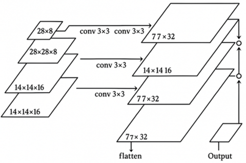
where, the function denoting the semantic segmentation model is called $f_{semantic}$, the input image is called I, and the semantic segmentation model's parameters are called $\Theta_{semantic}$. Three phases of upsampling are performed, beginning at the deepest FPN level (at the 1/32 size). Figure 3 shows how to make a 1/4 scale feature map. Each upsampling stage comprises of two bilinear upsampling, Group Norm, ReLU, and 3×3 convolution. For the 1/16, 1/8, and 1/4 FPN scales, the same method is repeated.
Figure 3. Semantic segmentation process
A collection of feature maps with the same scale of 1/4 constitutes the result, and these feature maps are then added one by one. Softmax, a final 1×1 convolution, and four bilinear upsampling are used to construct the per-pixel class labels at the original image resolution.
4.2.3 Instance segmentation
Once the types of lesions are identified, instance segmentation can be applied to distinguish individual instances of each lesion type. Instance segmentation assigns a unique label to each instance of a lesion, enabling precise localization and counting of lesions within the retinal image. The instance segmentation model should be trained on annotated retinal images with instance-level labels for each lesion type.
Let $I$ denote the instance segmentation output, which is a set of instance masks indicating the pixel-wise segmentation of each object instance. It is represented as follows:
$I=f_{ {instance }}\left(I ; \Theta_{{instance }}\right)$ (6)
where, $\Theta_ {instance }$ are the parameters of the instance segmentation model, and $f_ {instance }$ is the function representing the instance segmentation model.
4.2.4 Merging using heuristics
Panoptic segmentation is a technique that combines the output of instance and semantic segmentation into a single segmentation map that includes both "stuff" and "things." This is represented as follows:
$P=\{(S, I)\}$ (7)
The panoptic segmentation output is denoted as P, and each tuple $(S, I)$ represents the semantic and instance segmentation results of the image.
To create a thorough segmentation map for retinopathy, the results of instance and semantic segmentation are integrated. To do this, the instance segmentation masks which offer comprehensive details on specific lesion instances are combined with the semantic segmentation map, which offers a high-level summary of lesion varieties. The integration process may involve techniques such as overlaying instance segmentation masks onto the semantic segmentation map or using conditional probability distributions to refine segmentation boundaries.
4.3 Panoptic FPN
The model uses an encoder-decoder architecture with FPN and a novel merging algorithm. The following steps are performed as follows:
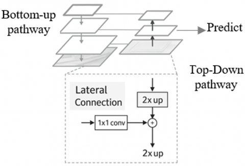
Through lateral connections and a top-down methodology, it combines low-resolution, semantically strong features with high-resolution, semantically weak data, as shown in Figure 4. This feature pyramid has extensive semantics at all levels and can be quickly built from a single input image scale without reducing textual strength, performance, or space.
Figure 4. FPN
The Panoptic FPN's bottom-up route is in charge of constructing a feature pyramid out of the feature maps that the backbone network has retrieved. This pyramid allows the network to leverage multi-scale information, capturing both detailed spatial information and high-level semantic features.
4.3.1 Backbone feature extraction
The backbone network will be represented by $\mathcal{B}$. The backbone network retrieves a series of feature maps at various network levels given an input image I.
$\left\{C_1, C_2, C_3, C_4\right\}=B(I)$ (8)
where, $C_i$ represents the feature map at level $i$ of the backbone.
4.3.2 Bottom-up pathway
The bottom-up pathway involves applying convolutional transformations to each feature map $C_i$ to create a set of feature maps $P_i$ for the feature pyramid.
Initial Feature Maps from Backbone Given the feature maps $C_1, C_2, C_3, C_4$, the bottom-up pathway creates feature maps $\left\{P_1, P_2, P_3, P_4\right\}$.
$P_i={Conv}_{ {bottom-up }}^i\left(C_i\right)$ (9)
where, $Conv_{ {bottom-up }}^i$ represents a convolutional operation applied to the feature map $C_i$ at level i.
Fusion in bottom-up pathway Each feature map $P_i$ at a given level i can be expressed as:
$P_i=W_i * C_i$ (10)
where, * denotes the convolution operation and $W_i$ are the learnable convolutional weights at level i. This operation can be formalized as:
$P_i=\sigma\left(W_i * C_i+b_i\right)$ (11)
where, $\sigma$ is an activation function and $b_i$ is the bias term.
Combining Feature Maps To produce the ultimate feature maps for the bottom-up approach, each feature map $P_i$ is concatenated or added based on upsampling or pooling operations:
$P_i={Concat}\left(P_{i+1}^{\uparrow}, {Conv}\left(C_i\right)\right)$ (12)
where, $P_{i+1}^{\uparrow}$ denotes the upsampled feature map from the higher level i+1 and ${Conv}\left(C_i\right)$ is the convolution applied to the feature map at level i.
Full feature pyramid Finally, the set of feature maps for the entire feature pyramid is: $\left\{P_1, P_2, P_3, P_4\right\}$. The bottom-up pathway in Panoptic FPN is essential for constructing a multi-scale feature pyramid from backbone feature maps. Accurate panoptic segmentation depends on the integration of multi-scale information, which is achieved by the use of these feature maps in the top-down route and lateral linkages.
4.3.3 Top-down pathway
Using a top-down pathway, fused feature maps are produced by upsampling higher-level feature maps and adding them to lower-level feature maps via lateral connections. Let's denote the top-down feature maps as $\left\{T_1, T_2, T_3, T_4\right\}$. The top-down pathway can be represented as follows.
$T_i={Upsample}\left(T_{i+1}\right)+{Conv}\left(P_i ; \Theta_{t o p-d o w n}\right)$ (13)
where, Upsample denotes upsampling operation, and $\Theta_{t o p-d o w n}$ represents the parameters of the convolutional layers.
4.3.4 Semantic segmentation head
The semantic segmentation head takes the top-down feature maps $T_i$ and produces semantic segmentation predictions $S_i$ at each level. The semantic segmentation head can be represented as follows.
$S_i={Conv}\left(T_i ; \Theta_{ {semantic }}\right)$ (14)
where, $\Theta_{ {semantic }}$ represents the parameters of the convolutional layers.
4.3.5 Instance segmentation head
The segmentation head takes the top-down feature maps $T_i$ and produces instance segmentation predictions $I_i$ at each level. The instance segmentation head can be represented as follows.
$I_i={Conv}\left(T_i ; \Theta_{ {instance }}\right)$ (15)
where, $\Theta_{ {instance }}$ represents the parameters of the convolutional layers.
4.3.6 Hybrid upsampling for accurate pixel labeling
To ensure that the segmentation outputs match the input image’s resolution, the proposed method utilizes hybrid upsampling. After feature extraction from the backbone network, the upsampling process enlarges the feature map through multiple stages of bilinear upsampling, followed by convolution and normalization layers, to generate per-pixel class labels. This hybrid technique effectively combines the detailed local features from the shallow layers of ResNet-50 with the global context captured at deeper layers, resulting in fine-grained pixel-level segmentation.
4.3.7 Panoptic segmentation integration
Finally, the semantic and instance segmentation predictions $S_i$ and $I_i$ are integrated to generate the panoptic segmentation output. The integration process can involve merging $S_i$ and $I_i$ based on pixel-wise classification scores and instance bounding boxes.
4.3.8 Lateral convolution
Prior to being integrated, lateral connections guarantee that feature maps from various levels have an equal number of channels.
$L_i={Conv}_{\text {lateral }}^i\left(P_i\right)=\sigma\left(W_i^L * P_i+b_i^L\right)$ (16)
where, $L_i$ is the output of the lateral convolution at level I; $W_i^L$ are the learnable weights for the lateral convolution; $b_i^L$ lateral convolution's bias term is denoted by L, while its activation function is represented by σ.
4.4 Pseudocode of panoptic FPN
|
def panoptic_fpn(image): Args: Image: The input image. Returns: The panoptic segmentation of the image. # 1. Encoder-decoder architecture. features = encoder(image) predictions = decoder(features) # 2. FPN. fpn_features = fpn(features) # 3. Region Proposal Network (RPN). proposals = rpn(fpn_features) # 4. Mask head. masks = mask_head(proposals) # 5. Merging algorithm. panoptic_segmentation = merge (predictions, masks) return panoptic_segmentation |
4.5 Loss function and hyperparameter tuning
The network was optimized by combining binary cross-entropy loss for instance segmentation with cross-entropy loss for semantic segmentation. The instance segmentation branch also utilized IoU loss to ensure precise localization of lesions within the SD-OCT images. Standard optimization techniques like Adam were used to optimize these loss functions, and learning rates were modified in response to the model's performance during training. Through iterative refinement and feedback from validation, hyperparameters such as learning rate, batch size, and filter sizes were adjusted.
4.6 Classification
The Deep Residual Learning network (Res-Net-50) is used to classify the images into object categories. The network learns a variety of features from the images. Res-Net-50 created feature maps, which were supplied to the panoptic field head. The bounding box predicts the class ID of the corresponding pixel. Semantic segmentation employs the same border box properties to reduce the number of parameters and network interference time. The outputs of instance and semantic segmentation are combined to get the final segmentation results. The panoptic segmented image is sent into ResNet-50's residual blocks and convolutional layers. The network structure is mathematically represented as a series of transformations as follows.
$x_{l+1}=F\left(x_l,\left\{w_l\right\}\right)+x_l$ (17)
where,
The following represents each residual block in ResNet-50.
$y={ReLU}\left(B N\left({Conv}\left(x, W_1, b_1\right)\right)\right)+x$ (18)
where,
After passing through multiple layers and residual blocks, the high-dimensional feature maps are reduced using global average pooling.
$z=\frac{1}{H \times W} \sum_{i=1}^H \sum_{j=1}^W y_{i j}$ (19)
The feature map's height and breadth are denoted by H and W. A Fully Connected (FC) layer is then applied to the pooled feature vector $z$ in order to transfer the features to the categorization space.
$f=W_{f c} z+b_{f c}$ (20)
where,
To generate a distribution of probabilities over each of the three groups (Normal, Abnormal, and Moderate), the output vector $f$ is subjected to a softmax function.
$\widehat{y_l}={Softmax}\left(f_i\right)=\frac{e^{f_i}}{\sum_j e^{f_i}}$ (21)
where,
The final classification decision is based on the highest probability from the softmax output:
${Class}(I)=\arg \max_i \widehat{y}_i$ (22)
where, $\arg \max _i \widehat{y}_l$ yields the greatest value's index i in the probability distribution $\widehat{y_l}$.
Using an encoder-decoder architecture, the initial step is obtaining features from the image itself. While the decoder reconstructs the images using the characteristics that the encoder has extracted, the encoder extracts features from the image at various sizes. Both semantic and instance segmentation benefit from the model's ability to extract features with different levels of specificity.
The second phase involves extracting characteristics from an image at various scales using the FPN. It is a method that enables the model to extract characteristics at various scales from a single input image. Both instance and semantic segmentation benefit from this as it gives the model a better understanding of the context of the items in the image.
Using the RPN, the third step is to suggest areas of interest in the image that are probably home to items. This method predicts the bounding boxes of objects in an image using a CNN network. This enables the model to recognize things in the image with speed and efficiency.
The fourth step is to predict masks for the objects that are RPN recommended the use of a mask head. Mask head is a method that uses the CNN to forecast pixel-level masks for objects in images. This enables the model to recognize object boundaries in the image with accuracy.
To create a panoptic segmentation, the semantic and instance segmentation predictions are combined using a merging algorithm in the last step.
The merging algorithm is a technique that uses a graph-based approach to merge the pixels of the image into objects. This enables the model to provide a single, cohesive representation of the image that incorporates the object-level detail of the image, which shows the location of each item, as well as the semantic content of the image.
5.1 Pseudocode for training ResNet-50 on OCT images
ResNet-50 with its deep architecture and residual learning, is well-suited for classifying OCT images. By enabling the model to learn residual functions, it successfully manages the difficulties associated with deep network training, making it an excellent tool for OCT image processing tasks like recognizing and categorizing diseases like Purtscher's Retinopathy.
BEGIN
DISPLAY (performance)
END
5.2 Pseudocode of Panoptic FPN followed by ResNet-50 for classification
Integrating the segmented results from the FPN into a ResNet-50 classification pipeline for OCT images involves several steps. Below is a detailed pseudocode, incorporating mathematical formulas, for training a ResNet-50 model using the segmented OCT images as input.
Step 1: Preprocessing and Loading Data
Step 2: Apply Panoptic FPN for Segmentation
$S_i=A P P L Y_{-} P A N O P T I C_{-} F P N\left(X_i\right)$
$S=\left\{S_i\right\}_{i=1}^N$
Step 3: Define ResNet-50 Architecture
Model architecture is predefined with 50 layers using the residual blocks.
Step 4: Compile the Model
Loss function: Categorical Cross-Entropy:
$L=-\sum_{c=1}^C y_c \log \left(\widehat{y_c}\right)$
Step 5: Train the Model
Train the model with segmented images S and labels y:
$\begin{gathered} { model. } { TRAIN }(S, y, { epochs }=50, { batch_{-}size }=32, \\ { validation_{-}split }=0.2)\end{gathered}$
Step 6: Evaluate the Model
$T=\left\{\left(X_{ {test }, j}, y_{ {test }, j}\right)\right\}_{j=1}^M$
For each test image $X_{ {test }, j}$:
$S_{ {test }, j}=A P P L Y_{-} P A N O P T I C_{-} F P N\left(X_{ {test } . j}\right)$
Utilizing the test labels and segmented test images, assess the model:
$performance= model. E V A L U A T E\left(s_{{test }}, y_{ {test }}\right)$
Step 7: Display Results
DISPLAY(performance)
This pseudocode outlines the process of using Panoptic FPN for segmentation followed by ResNet-50 for classification, integrating detailed mathematical operations at each step.
Purtscher's Retinopathy is a rare but devastating eye condition that mostly affects young or middle-aged men and is brought on by trauma. A PR clinical diagnosis has been proposed. Three of the five conditions listed below must be met.
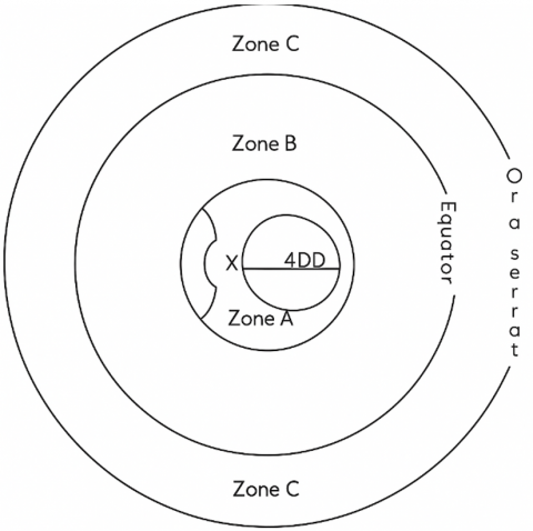
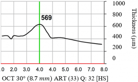
The level of retinal degeneration in PR is determined, as shown in Figure 5. To analyze the disease, the retina is divided into three zones such as A, B, and C respectively. Zone A is with a radius of four-disc diameters and 2/3 of cases arise here. Zone B extends outside A. Zone C is anterior to Zone B and it is affected rarely. Panoptic segmentation assigns a class label to each pixel through its semantic process and the instance segmentation segments the object instance.
PR, occlusion occurs at the level of pre-capillary arterioles, which have a diameter of roughly 45 m. This causes whiteness in the areas of the distal capillary beds and typically perfused retina nearer to the arterioles. Occlusions close to the pre-capillary arterioles cause confluent whitening, similar to a branch retinal artery occlusion, but occlusions further away cause cotton wool patches that conceal the underlying arteries.
As shown in Figure 6, there are several etiologies to take into consideration when diagnosing peripapillary cotton wool patches with associated macular retinal whitening, including vascular, metabolic, inflammatory, autoimmune, traumatic, viral, and hematologic. Every occurrence was symptomatic, exhibiting either a decrease in vision field or acuity, or both. Retinal pigment epithelium atrophy and optic disc pallor were the most common chronic symptoms. The diagnosis of PR was validated by the patient's manifestation of Purtscher Flecken in the context of C5a hypercomplementemia.
Figure 5. Retinal Zones involvement in PR
Figure 6. The retinal nerve fiber layer becomes thinner as a result of cotton wool patches [6]
Figure 7. Results reflect the best, median, and worst performances
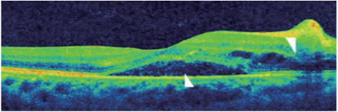
Figures 7a to 7c show the best case, Figures 7d to 7f show the median case, and Figures 7g to 7i show the worst case of the obtained results through the proposed approach. The optimum best performance occurs when the OCT image displays the layers of the retina. Its Dice Coefficient is > 0.90 and IoU > 0.85. The retinal layers are precisely segmented by the model, which also detects anomalies such as retinal hemorrhages and whitening. The segmentation delineates the impacted areas, closely matching the ground reality.
The OCT image with mild retinal abnormalities and considerable noise is in the median performance. Metrics: Dice coefficient between 0.70 and 0.80, IoU between 0.60 and 0.75. With certain inconsistencies, the model offers a comparatively accurate segmentation. While it accurately detects the main characteristics of Purtscher's retinopathy, noise or poorly defined boundaries may cause it to ignore minute details or add a little segmentation error.
(a) sub-retinal detachment
(b) Macular edema
(c) Purtscher’s flecken
(d) Infected Purtscher’s retina analysis
Figure 8. Results of Purtscher’s Retinopathy analysis
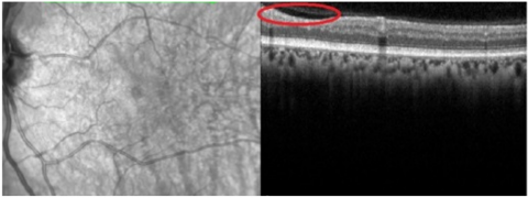
When the OCT image exhibits extreme retinal distortion, artifacts, or noise, it is said to have the lowest performance. Dice coefficient < 0.60 and IoU < 0.50. The segmentation of anomalies and retinal layers by the model is not very accurate. Noise and artifacts can have a significant impact on predictions, resulting in a low overlap with the ground truth. In certain situations, the model is unable to offer meaningful diagnostic data. The spectral-domain optical coherence is shown in Figure 8. Left eye tomography shows a subfoveal neurosensory separation with rupture of the ellipsoid zone, along with significantly affected inner retinal areas and characteristic Purtscher Flecken (arrow).
The FPN results on OCT segmentation involve evaluating different performance metrics across several test images. This includes metrics like Intersection over Union (IoU), Dice coefficient, pixel accuracy, precision, recall, and F1 score.
1. IoU (Intersection over Union): It determines the degree to which the ground truth and the expected segmentation overlap.
$I o U=\frac{T P}{T P+F P+F N}$ (23)
2. Dice Coefficient: A similar measure to IoU, but it tends to be more sensitive to small objects. It is defined as follows.
$Dice \ Coefficient=\frac{2 \times T P}{2 \times T P+F P+F N}$ (24)
3. Pixel Accuracy: The percentage of all pixels that were correctly predicted.
$Pixel\ Accuracy=\frac{\ { No.\ of\ Correctly\ Predicted\ Pixels }}{ { Total\ no.of\ Pixels }}$ (25)
4. Precision: The ratio of correctly predicted positive outcomes to all predicted positive outcomes.
$Precision =\frac{T P}{T P+F P}$ (26)
5. Recall: The ratio of true positive forecasts to all real positives.
$Recall =\frac{T P}{T P+F N}$ (27)
Interpretation of Table 2 is as follows.
To improve the statistical validity and generalizability of the results, the sample size of PR patients must be increased for further research. A larger dataset would enable more thorough research and a more accurate depiction of the features of the illness. Furthermore, to prevent bias and guarantee that the results apply to both male and female populations, equal gender representation is vital. A more thorough knowledge of the disease's course and its effects on various phases would also be possible with the inclusion of a wider variety of disease severity levels. In addition to increasing the prediction models' accuracy, these actions would help develop more individualized and efficient methods for diagnosing and treating PR.
The PR segmentation findings are shown in Figure 9, along with an evaluation of the IOUs. It is found that the model performs better when segmented photos are used as an extra source of training data.
Figure 9. IOU (Intersection over Union) of PR segmentation over epochs
Table 2. Comparison of FPN results on SD-OCT segmentation
|
Image ID |
IoU |
Dice Coefficient |
Pixel Accuracy |
Precision |
Recall |
F1 Score |
|
Image 1 |
0.85 |
0.92 |
0.95 |
0.9 |
0.88 |
0.89 |
|
Image 2 |
0.78 |
0.85 |
0.9 |
0.84 |
0.82 |
0.83 |
|
Image 3 |
0.6 |
0.75 |
0.8 |
0.7 |
0.65 |
0.67 |
|
Image 4 |
0.92 |
0.95 |
0.98 |
0.94 |
0.91 |
0.93 |
|
Image 5 |
0.5 |
0.67 |
0.75 |
0.6 |
0.55 |
0.57 |
|
Image 6 |
0.83 |
0.89 |
0.93 |
0.87 |
0.85 |
0.86 |
|
Image 7 |
0.72 |
0.8 |
0.85 |
0.78 |
0.74 |
0.76 |
|
Image 8 |
0.68 |
0.77 |
0.82 |
0.75 |
0.7 |
0.72 |
|
Image 9 |
0.9 |
0.93 |
0.97 |
0.92 |
0.89 |
0.91 |
|
Image 10 |
0.55 |
0.71 |
0.78 |
0.65 |
0.6 |
0.62 |
Table 3. Comparison of OCT segmentation with competitive methods
|
Metrics |
FPN (Panoptic FPN) |
U-Net |
SegNet |
DeepLabV3 |
PSPNet |
|
Mean IoU |
0.88 |
0.71 |
0.68 |
0.7 |
0.72 |
|
Mean Dice |
0.92 |
0.8 |
0.77 |
0.79 |
0.81 |
|
Mean Pixel Accuracy |
0.97 |
0.85 |
0.83 |
0.84 |
0.86 |
|
Mean Precision |
0.99 |
0.77 |
0.74 |
0.76 |
0.78 |
|
Mean Recall |
0.98 |
0.74 |
0.71 |
0.81 |
0.75 |
|
F1 Score |
0.93 |
0.75 |
0.72 |
0.74 |
0.76 |
In particular, the model converges somewhat quicker when merging segmented images than it does with training segmentation data, especially in the initial few epochs. To be more precise, the model's initial epoch performs nearly identically to the 10th epoch when taking the validation set's performance into account. This phenomenon indicates that there is a substantial association between the segmentation task and the characteristics used for object detection. Table 2 aids in evaluating the FPN model's performance on OCT segmentation tasks and pointing out its advantages and disadvantages in various situations.
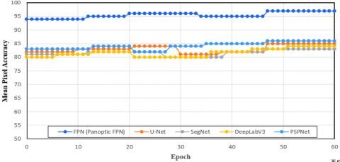
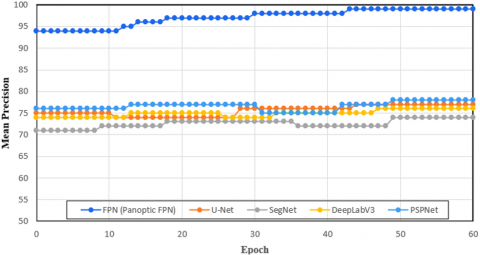
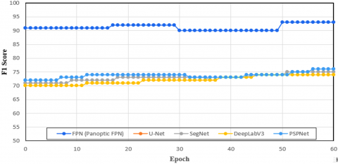
Table 3 provides a detailed comparison of the performance of different segmentation methods (Panoptic FPN, U-Net, SegNet, DeepLabV3, and PSPNet) on OCT images across several performance metrics.
The U-Net design, which was proposed by Karn and Abdull [21], is a common method for segmenting OCT images, particularly in situations where pixel-level classification is essential. Both fine-grained geographical features and high-level contextual information may be captured by its encoder-decoder structure with skip connections. When it comes to complicated, overlapping lesions like those found in PR, U-Net's capacity to differentiate distinct diseased characteristics is limited by its emphasis on semantic segmentation. This presents a major obstacle to the identification of retinal diseases because precise lesion-level segmentation is essential. To provide a more thorough knowledge of retinal defects, Panoptic FPN, on the other hand, combines instance and semantic segmentation, enabling it to recognize and distinguish particular lesions such as hemorrhages and cotton-wool patches. Additionally, the proposed Panoptic FPN's multi-scale feature extraction, which makes use of the FPN, improves its capacity to identify dispersed and tiny lesions, which is a drawback of U-Net in intricate retinal structures.
To improve segmentation performance in scene parsing tasks, PSPNet uses a global pooling layer in conjunction with a Pyramid Scene Parsing (PSP) module to gather context from various spatial scales [22]. The local, specific qualities that are essential for precise lesion diagnosis in retinal images are not sufficiently addressed, even though this is helpful for comprehending global scene contexts. In contrast, the proposed Panoptic FPN employs both instance and semantic segmentation, enabling the differentiation of individual lesions and enhancing the precision of detection in conditions such as PR, where accurate localization of lesions is crucial.
Panoptic FPN consistently performs the best across all metrics, demonstrating its effectiveness and robustness in OCT image segmentation. PSPNet shows competitive performance, slightly trailing behind Panoptic FPN, making it a strong contender. U-Net and DeepLabV3 both methods show moderate performance, proving their reliability but indicating room for improvement compared to Panoptic FPN and PSPNet. SegNet shows the least performance across all metrics, suggesting it is less suitable for SD-OCT segmentation tasks compared to the other methods to diagnose PR. Additionally, the architecture of the proposed Panoptic FPN is better suited to complicated retinal structures, whilst PSPNet's global scene parsing technique may easily overlook minor and overlapping lesions. As a result, Panoptic FPN provides a better model for tracking and detecting retinal problems early.
DeepLab V3 employs Atrous Spatial Pyramid Pooling (ASPP) for multi-scale feature extraction in order to better capture context at different resolutions [23]. DeepLab V3 has limits in retinal image segmentation, where minute and subtle lesions (typical of PR) need to be properly located, despite being successful for large-scale scene parsing. Furthermore, DeepLab V3 cannot independently detect distinct problematic components, instead concentrating on semantic segmentation. However, the proposed Panoptic FPN is more capable since it offers both instance and semantic segmentation. Panoptic FPN's multi-scale feature extraction provides better diagnostic capabilities for retinal disorders like PR by more successfully catching both major retinal abnormalities and fine-grained lesions.
To diagnose PR using SD-OCT images, the proposed Panoptic FPN outperforms U-Net [21], PSPNet [22], and DeepLab V3 [23] because it integrates instance and semantic segmentation, allowing it to recognize and differentiate certain lesions. PSPNet's emphasis on global image parsing renders it less successful at recognizing tiny or dispersed lesions, like those present in PR, whereas U-Net performs well for segmentation tasks but has trouble with complex overlapping lesions. Similar to this, the ASPP method for multi-scale detection in DeepLab V3 is effective for comprehending scenes but lacks the granularity needed to differentiate minute retinal lesions that are typical of PR. The proposed Panoptic FPN is especially well-suited for identifying the delicate, intricate, and dispersed lesions in PR because to its dual segmentation technique and multi-scale feature extraction, which yields more precise, localized, and clinically useful results.
Figure 10. Comparison of mean IOU
Figure 11. Comparison of mean dice coefficient
Figure 12. Comparison of mean pixel accuracy
Figure 13. Comparison of mean precision
Figure 14. Comparison of mean recall
Figure 15. Comparison of F1 score
The proposed method for diagnosing PR using panoptic segmentation offers several practical implications in a clinical setting. In terms of computational efficiency, the system is designed to operate with reasonable speed, benefiting from the use of ResNet-50 as a backbone, which strikes a balance between performance and computational cost. While the system may not yet operate in real-time in resource-constrained environments, with optimized hardware and further model refinement, real-time processing could be achievable. The system’s outputs, particularly the panoptic segmentation maps, can be presented in a clinically interpretable format through color-coded heatmaps, where specific lesions are highlighted for the ophthalmologist’s review. This enables visual confirmation of the machine's findings while also providing the segmentation of individual lesions, which aids in diagnosis. To further enhance interpretability, the system could include confidence scores or probability maps to reflect the certainty of the predictions made.
However, there are potential challenges in adopting such a system in clinical practice. The requirement for sizable annotated datasets for efficient model training is one major obstacle. The availability of sufficiently diverse, well-annotated datasets that cover different demographic groups, imaging conditions, and disease severities is a significant barrier. Without such data, the model's accuracy and generalizability may be limited. Additionally, there is a risk of over-reliance on automated systems, potentially leading to misdiagnoses if the model’s predictions are not cross-validated by experienced ophthalmologists. Clinicians must maintain a supervisory role in the diagnostic process, using the system as a supportive tool rather than as a replacement for expert judgment. To mitigate this, hybrid systems that combine machine learning outputs with clinician insights would be the most effective approach.
The primary limitation of this study is the small, imbalanced dataset, particularly with only 10 Purtscher-like Retinopathy (PR) cases (9 women and 1 man), which restricts the model’s generalizability. The model may also suffer from overfitting due to the limited number of PR cases and class imbalance. Additionally, the model is tailored for PR and may struggle to generalize to other retinal diseases, which often present different lesion types and severities.
To address these limitations, future studies should focus on collecting a larger, more diverse dataset with balanced gender, age, and disease severity. Incorporating OCT alongside fundus photography to improve lesion detection. Exploring transformer-based models and hybrid CNN-transformer architectures for better feature extraction. These advancements will enhance the model's accuracy, generalizability, and clinical applicability.
The panoptic segmentation is used for its potential to identify PR in the proposed research. It is a peculiar eye disease marked by blockages in the retinal blood vessels that cause vision loss. The high-resolution cross-sectional retinal images acquired from SD-OCT are evaluated using this method. Automating the examination of these images by panoptic segmentation shows promise for quicker and more reliable diagnosis. Furthermore, compared to conventional techniques, it may be more accurate in identifying the distinctive hyperreflective lesions and Purtscher Flecken in the retina by combining several segmentation techniques. However, several issues must be resolved. First and foremost, it is imperative to train the Panoptic Segmentation algorithm on huge datasets of PR patients. Furthermore, these algorithms must be interpreted in a way that allows ophthalmologists to comprehend the logic behind the diagnosis and continue to have faith in the technology. Also, clinical studies are required to confirm the precision and efficacy of panoptic segmentation in practical contexts. The possible advantages of Panoptic FPN segmentation outweigh these difficulties.
[1] Teussink, M.M., Donner, S., Otto, T., Williams, K., Tafreshi, A. (2019). State-of-the-art commercial spectral-domain and swept-source OCT technologies and their clinical applications in ophthalmology. Heidelberg Engineering, 1-19.
[2] Hamoudi, H., Nielsen, M.K., Sørensen, T.L. (2018). Optical coherence tomography angiography of Purtscher retinopathy after severe traffic accident in 16-year-old boy. Case Reports in Ophthalmological Medicine, 2018(1): 4318354. https://doi.org/10.1155/2018/4318354
[3] Lin, Y.C., Yang, C.M., Lin, C.L. (2006). Hyperbaric oxygen treatment in Purtscher’s retinopathy induced by chest injury. Journal of the Chinese Medical Association, 69(9): 444-448. https://doi.org/10.1016/S1726-4901(09)70289-8
[4] Agrawal, A., McKibbin, M.A. (2006). Purtscher’s and Purtscher-like retinopathies: A review. Survey of Ophthalmology, 51(2): 129-136. https://doi.org/10.1016/j.survophthal.2005.12.003
[5] Haq, F., Vajaranant, T.S., Szlyk, J.P., Pulido, J.S. (2002). Sequential multifocal electroretinogram findings in a case of Purtscher-like retinopathy. American Journal of Ophthalmology, 134(1): 125-128. https://doi.org/10.1016/S0002-9394(02)01474-5
[6] Piccolino, F.C., de La Longrais, R.R., Ravera, G., Eandi, C.M., Ventre, L., Manea, M. (2005). The foveal photoreceptor layer and visual acuity loss in central serous chorioretinopathy. American Journal of Ophthalmology, 139(1): 87-99. https://doi.org/10.1016/j.ajo.2004.08.037
[7] Battista, M., Cicinelli, M.V., Starace, V., Lattanzio, R., Bandello, F. (2020). Purtscher-like features in new-onset diabetic retinopathy. Acta Diabetologica, 57(3): 377-379. https://doi.org/10.1007/s00592-019-01401-x
[8] Agrawal, A., McKibbin, M. (2007). Purtscher’s retinopathy: epidemiology, clinical features and outcome. British Journal of Ophthalmology, 91(11):1456-1459. https://doi.org/10.1136/bjo.2007.117408
[9] Tripathy, K., Patel, B.C. (2023). Purtscher Retinopathy. In StatPearls. https://www.ncbi.nlm.nih.gov/books/NBK542167/.
[10] Pinto, C., Fernandes, T., Gouveia, P., Sousa, K. (2022). Purtscher-like retinopathy: Ocular findings in a young woman with chronic kidney disease. American Journal of Ophthalmology Case Reports, 25: 101301. https://doi.org/10.1016/j.ajoc.2022.101301
[11] Purtscher's Retinopathy. https://en.wikipedia.org/wiki/Purtscher%27s_retinopathy, access on Jun. 5, 2024.
[12] Aldhefeery, N., Aldhafiri, D., Fathy, M., Kumaran, S., Abdelbadie, M. (2023). Bilateral Purtscher-like retinopathy: A case report in a patient with pre-eclampsia and post intrauterine fetal demise. International Journal of Surgery Case Reports, 113: 109072. https://doi.org/10.1016/j.ijscr.2023.109072
[13] Massa, R., Vale, C., Macedo, M., Furtado, M.J., Gomes, M., Lume, M., Meireles, A. (2015). Purtscher-like retinopathy. Case Reports in Ophthalmological Medicine, 2015(1): 421329. https://doi.org/10.1155/2015/421329
[14] Xiao, W., He, L., Mao, Y., Yang, H. (2018). Multimodal imaging in Purtscher retinopathy. Retina, 38(7): e59-e60. https://doi.org/10.1097/IAE.0000000000002218
[15] Sokol, J.T., Castillejos, A., Sobrin, L. (2022). Purtscher-like retinopathy following a bowel movement. American Journal of Ophthalmology Case Reports, 26: 101560. https://doi.org/10.1016/j.ajoc.2022.101560
[16] Benvenuto, F., Guillen, S., Marchiscio, L., Falbo, J., Fandiño, A. (2021). Purtscher-like retinopathy in a paediatric patient with haemolytic uraemic syndrome: A case report and literature review. Archivos de la Sociedad Española de Oftalmología (English Edition), 96(11): 607-610. https://doi.org/10.1016/j.oftale.2020.10.007
[17] Zhang, W.F., Dai, R.P., Chen, Y.X. (2024). Bilateral purtscher-like retinopathy associated with antiphospholipid syndrome and thrombotic microangiopathy. Ophthalmology Retina, 8(11): e39. https://doi.org/10.1016/j.oret.2024.03.021
[18] Rothbächer, J., Bolz, M., Khalil, H. (2025). Case report: Purtscher-like Retinopathy in a Patient after otorhinolaryngological surgery. American Journal of Ophthalmology Case Reports, 37: 102265. https://doi.org/10.1016/j.ajoc.2025.102265
[19] Blodi, B.A., Johnson, M.W., Gass, J.D.M., Fine, S.L., Joffe, L.M. (1990). Purtscher's-like retinopathy after childbirth. Ophthalmology, 97(12): 1654-1659. https://doi.org/10.1016/S0161-6420(90)32365-5
[20] Intagliata, E., Giugno, S., Vizzini, C., Cacciola, R.R., Vecchio, R., Vecchio, V. (2022). An unusual association between pancreatic cancer and Purtscher-like retinopathy: Presentation of a unique case. International Journal of Surgery Case Reports, 96: 107338. https://doi.org/10.1016/j.ijscr.2022.107338
[21] Karn, P.K., Abdulla, W.H. (2024). Advancing Ocular Imaging: A hybrid attention mechanism-based U-Net Model for precise segmentation of sub-retinal layers in OCT images. Bioengineering, 11(3): 240. https://doi.org/10.3390/bioengineering11030240
[22] Liu, Y., Nezami, F.R., Edelman, E.R. (2024). A Transformer-based pyramid network for coronary calcified plaque segmentation in intravascular optical coherence tomography images. Computerized Medical Imaging and Graphics, 113: 102347. https://doi.org/10.1016/j.compmedimag.2024.102347
[23] Mukherjee, S., De Silva, T., Duic, C., Jayakar, G., Keenan, T.D., Thavikulwat, A.T., Cukras, C. (2024). Validation of deep learning-based automatic retinal layer segmentation algorithms for AMD with two SD-OCT devices. Ophthalmology Science, 5(3): 100670. https://doi.org/10.1016/j.xops.2024.100670