Abdullah Yagiz![]() | Sinan Uguz*
| Sinan Uguz*![]()
© 2025 The authors. This article is published by IIETA and is licensed under the CC BY 4.0 license (http://creativecommons.org/licenses/by/4.0/).
OPEN ACCESS
Although Turkey ranks first in the world in terms of raisin exports, it ranks fourth in revenue. The main reason for this problem is that the quality of exported raisins does not meet the desired level. In this study, an intelligent real-time system was developed to determine suitability for export by classifying raisins according to color and capstem amount according to the criteria of TS 3411. A dataset of 2336 Sultana raisins was created and expanded to 10,544 images using data augmentation techniques such as exposure adjustment, rotation, and noise addition. These techniques not only increased the dataset size but also significantly improved the model performance, as evidenced by the remarkable success of the CNN models with an average mAP of 98.8%. The images were evaluated in real time in the developed GUI software and their compliance with the standard was determined. The study is the first of its kind to classify and detect raisins according to the standard TS 3411 using an intelligent real-time system.
object detection, classification, raisin, convolutional neural networks (CNN)
Grapes are one of the most widely produced fruits globally, with an annual production of approximately 75 million tons. Of this production, 53% is pressed for wine production, 44% is consumed as fresh table grapes, and 3% is discarded as unusable. Approximately 81% of the unpressed grapes are consumed as table grapes, while the remaining 19% are processed into raisins [1]. According to 2021 data, Turkey ranks first globally in raisin exports. Turkey holds a 28.5% share of the global raisin market, followed by the US and Iran with shares of 13.5% and 11.2%, respectively. However, Turkey ranks fourth in revenue per ton of raisins, generating $1862, behind the US, Greece, and Afghanistan [2]. Excessive pesticide use and the low quality of grapes are among the primary reasons for Turkey’s lower export revenue per unit compared to other countries. The quality of raisins is further impacted by deterioration during the drying stage and the presence of foreign substances during harvest [3].
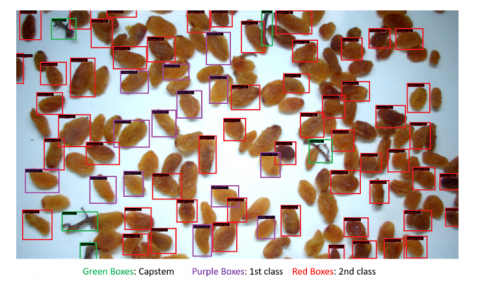
In Turkey, the classification criteria for seedless raisins, as well as the details of sampling, control, and marketing, are specified by the TS 3411 standard [4]. According to TS 3411, raisins chemically bleached before or after drying are referred to as "natural raisins." The intensity of light yellow, brown, and black colors in natural raisins significantly influences their quality. In export markets, light yellow raisins are generally preferred over other colors. Another important factor in exported seedless raisins is the amount of grape capstem or non-herbal substances. The standard additionally defines the permissible amount of grape capstem or non-herbal substances in 100 grams of seedless raisin samples.
Because raisins produced in Turkey are not consistently classified according to TS 3411 standards, the desired revenues cannot be achieved despite high export volumes. Finding technological solutions to address this issue is crucial. For instance, the moisture content of raisins is typically assessed through laboratory tests. However, the assessment of color, grape capstem, or non-herbal substances currently relies on manual evaluation in the field and factories. Developing intelligent systems to classify raisins according to specific standards could reduce costs and enhance export revenues.
In recent years, deep learning-based architectures have proven successful in classifying and detecting agricultural products. The size of agricultural products is a critical variable affecting the success of these architectures. Studies in the literature highlight applications on smaller products, such as grapes [5], soybean seeds [6], and olives [7], as well as on larger fruits, including melons [8], potatoes [9], and cucumbers [10]. Detecting small objects using deep learning-based architectures can be challenging due to difficulties in distinguishing them from other classes or background elements in the image [11]. This highlights the need to develop specialized solutions for small object detection.
Distinguishing studies that use image processing techniques from those based on deep learning highlights the superior performance of deep learning architectures. Mollazade et al. [12] classified raisins into four categories: green, green with tail, black, and black with tail, using images captured by a color CCD camera. Among the methods compared artificial neural networks (ANNs), support vector machines (SVMs), decision trees (DTs), and Bayesian networks (BNs)-ANNs achieved the highest accuracy at 96.33%. Yu et al. [13] conducted experiments on 480 images captured by an industrial camera to classify raisins based on their color and texture properties. Using the least squares support vector machine (LSSVM), they achieved an accuracy of approximately 95%. Çınar et al. [14] developed a computer vision system that distinguished between common food and goat raisin varieties in Turkey. Among logistic regression (LR), multi-layer perceptron (MLP), and SVM models compared, MLP demonstrated the best performance with an accuracy of 86.44%. Khojastehnazhand and Ramezani [15] evaluated the performance of bulk raisin systems by combining various texture feature algorithms with different modeling methods. The dataset was divided into three groups: good raisins, bad raisins, and other waste. Experiments were performed on combinations of these groups, resulting in 6 and 15 classes. The study concluded that the SVM classifier combined with gray level run length matrix (GLRM) features produced the most accurate classification results. Zhao et al. [16] proposed a deep learning-based segmentation algorithm to estimate the number of raisins. The primary strength of this algorithm is its ability to estimate the number of stuck raisins. The random forest (RF) and SVM models they employed for estimating raisin counts performed worse than the deep learning-based segmentation model.
The objective of this study is to develop a deep learning-based system to classify raisins by their color and capstem quantity in compliance with the TS 3411 seedless raisin standard. The proposed system seeks to automate quality control processes, improve export quality, and increase industrial efficiency. The specific contributions of this paper are as follows:
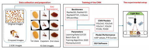
The processes depicted in Figure 1 were implemented to classify raisins in accordance with the TS 3411 standard. During the data collection and preparation phase, raisin samples captured using an industrial camera were individually cropped. This process resulted in a dataset containing 2,336 images of raisins. Subsequently, the dataset was expanded to 10,544 images using data augmentation techniques. Next, the performance of various state-of-the-art models (YOLOv5, YOLOv6, YOLOv7, YOLOX, FCOS, and TOOD) was evaluated. The experiments conducted with these models utilized the backbone networks and training parameters outlined in Figure 1. Upon completing the training process, the model achieving the highest performance was selected. Custom software was developed for the selected model, enabling real-time monitoring of the detected raisins. In the final phase of the study, a real-time system was integrated into the conveyor belt to classify raisins. These processes, which are part of the general experimental workflow, are elaborated upon in the following subsections.
2.1 Data collection and preparation
The raisins used in this study were sourced from a factory in Manisa, a province in Turkey's Aegean region. This factory processes export-quality Sultana raisins supplied by multiple farmers from across the region. Raisins were selected from batches delivered to the factory, ensuring a diverse representation of the Sultana raisin variety and avoiding bias toward any specific farm or producer.
During the imaging process, raisins were randomly placed on a white conveyor belt in 100-gram batches. The samples were mixed to simulate real-world conditions, ensuring the presence of both raisins and capstems. An industrial camera was positioned 25 cm above the conveyor belt to capture high-quality images. Fixed lighting conditions were used to ensure consistency and standardization throughout the imaging process. The captured images, originally sized at 1920x1080 pixels, were cropped to 240×135 pixels. This process resulted in a total of 2,636 cropped raisin images.
Figure 1. General operating diagram for experimental studies
Table 1. Number of classes in the dataset
|
Classes |
Data Augmentation Technique |
Original Data |
Augmented Data |
|
1st class |
Exposure, rotation, noise |
600 |
2400 |
|
2nd class |
1168 |
4672 |
|
|
Capstem |
868 |
3472 |
|
|
Total |
2636 |
10544 |
The dataset was labeled using Roboflow [17], an online platform for data annotation and augmentation. Roboflow supports multiple labeling formats, including COCO, Pascal VOC, and YOLO. For this study, YOLO format was used to train YOLOv5, YOLOv6, and YOLOv7 models, while the COCO format was employed to train FCOS, TOOD, and YOLOX models.
Data augmentation techniques are widely used in object detection applications within agricultural studies [18, 19]. These techniques improve estimation performance and help develop models that are less prone to overfitting [20]. Data augmentation was applied to each class of the dataset, and the resulting image counts are presented in Table 1. The original dataset consisted of 2,336 images distributed among three classes: 600 images of 1st class raisins, 1,168 images of 2nd class raisins, and 868 images of capstems. This distribution reflects the natural variability in Sultana raisins and was carefully designed to maintain balanced representation across all classes. Data augmentation techniques-such as exposure adjustment, rotation, and noise addition-were employed to expand the dataset to 10,544 images, preserving balanced class distributions.
In this study, the dataset was divided into three groups following data augmentation, with a ratio of 80-10-10 for training, validation, and testing, respectively. Similar ratios have been commonly applied in agricultural studies focused on disease detection [21-23].
2.2 Training of the CNN models
A general CNN structure consists of two main blocks: feature learning and fully connected layers. The feature learning block includes convolutional and pooling layers, where various matrix operations are performed to extract features from the input image. In the fully connected layers, the class of the input image is predicted through artificial neural network operations. CNN architectures were first introduced with LeNet-5 [24], followed by AlexNet [25], and subsequently evolved into numerous architectures that successfully address object detection problems. These architectures incorporate various convolutional operations, pooling methods, and diverse activation functions.
In this study, experiments were conducted using six state-of-the-art CNN models: YOLOv5, YOLOv6, YOLOv7, YOLOX, FCOS, and TOOD. Each model was tested with at least two different backbone networks. The best-performing networks are listed in Table 2 in Section 3.
The construction and training of the state-of-the-art models were implemented in Python 3.9 using PyTorch 1.12. The Adam optimizer and cross-entropy loss function were used for network training. The experiments were conducted on a workstation equipped with an Intel Xeon CPU, a 16GB Nvidia Quadro RTX5000GPU, and 16GB RAM. All input images were resized to match the network's input size requirements before training.
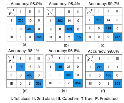
Figure 2. Confusion matrices of all the CNN models
(a) YOLOv5 (Backbone: CSPDarknet-x), (b) YOLOv6 (Backbone: EfficientRep-l), (c) YOLOv7 (Backbone: E-ELAN-x), (d) YOLOX (Backbone: CSPDarknet-x), (e) FCOS (Backbone: ResNeXt101), (f) TOOD (Backbone: ResNeXt101
The dataset was split into training, validation, and testing sets. First, 90% of the augmented data was randomly allocated as the training set, and the remaining 10% was used as the test set. From the training set, 10% was further separated to create a validation set. The data was then imported into the proposed network, and training parameters were configured. The model's parameters were as follows: batch size, 32; number of iterations, 50; initial learning rate, 0.0125; optimizer, SGD (Stochastic Gradient Descent); momentum, 0.9. Training was terminated after 400 epochs, and the network's accuracy and loss rates were calculated. Finally, a confusion matrix was generated to analyze the performance on the input data.
The performance of the state-of-the-art models was evaluated using classification metrics derived from the confusion matrix, as illustrated in Figure 2.
The confusion matrix was used to evaluate how effectively the state-of-the-art models classified classes 1, 2, and Capstem in the raisin images. A higher total sum of True Positive (TP) and True Negative (TN) values (highlighted in colored cells in Figure 2) indicates better model performance. In the confusion matrix, each column represents the instances of an actual raisin class, while each row represents the instances of a predicted raisin class.
While the confusion matrix provides valuable insights, it does not fully capture the performance of the models. By utilizing the values of TP, TN, False Positive (FP), and False Negative (FN) within the confusion matrix, performance metrics such as Accuracy, Precision, and Recall can be calculated. These metrics are defined in Eq. (1), Eq. (2), and Eq. (3), respectively, and provide a more comprehensive understanding of model performance.
Accuracy $=\frac{\mathrm{TP}+\mathrm{TN}}{\mathrm{TP}+\mathrm{TN}+\mathrm{FP}+\mathrm{FN}}$ (1)
Precision $=\frac{T P}{T P+F P}$ (2)
Recall $=\frac{T P}{T P+F N}$ (3)
Measuring object detection performance differs from evaluating classification performance. In this study, average precision (AP) was chosen to assess the performance of the models for the three different raisin classes. AP, as defined in Eq. (4), is widely utilized in the literature for object detection problems in agriculture [26-28].
$A P=\frac{1}{10}\left(A P_{.50}+A P_{.55}+A P_{.60}+\cdots+A P_{.95}\right)$ (4)
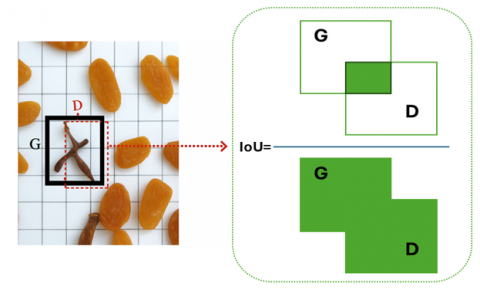
AP provides performance metrics for a single class. When there are multiple classes, mean average precision (mAP) is used instead of AP [29]. In this study, raisin classification involved three classes; therefore, the mAP value was employed to evaluate classification success. As illustrated in Figure 3, the ratio of the intersection of the ground truth (G) and default boxes (D) to their union is referred to as the intersection over union (IoU).
IoU takes values between 0 and 1, with higher values indicating better overlap between the ground truth (GT) and default boxes (DB). In this study, various mAP values were calculated for all state-of-the-art models, as presented in Table 2 in Section 3. Among these, the best results were achieved with mAP IoU=0.50.
Figure 3. Matching of default boxes with ground-truth
2.3 Experimental setup
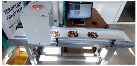
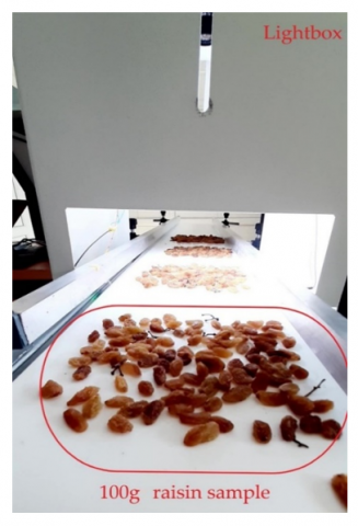
A conveyor belt system was designed for the real-time classification of raisins. The conveyor belt is 170cm long and 30cm wide, with an adjustable speed ranging from 1cm/s to 25cm/s across five levels. As illustrated in Figure 4, 100-gram raisin samples can be placed at intervals along the conveyor belt.
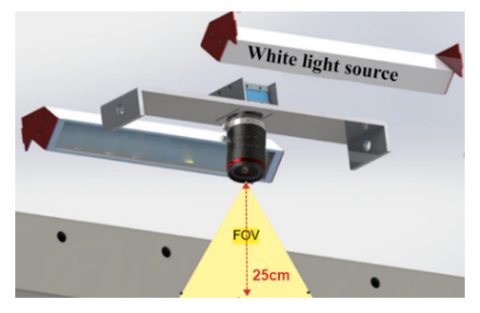
Figure 4. General operating diagram for experimental studies
Figure 5. Inside the light box
The light box integrated with the conveyor belt houses an Image Source DFK 37BUX290 industrial camera, a Fujinon DF6HA-1S 6mm lens, and two 24 V LED strip light sources. Industrial cameras with a high frame rate (Frames Per Second, FPS) are essential for capturing moving objects effectively. The camera used in this study operates at 140 FPS, ensuring that image quality is maintained even as the conveyor belt speed increases. According to the TS3411 standard, the quality criteria for 100-gram raisin samples must be met. Therefore, the camera lens was chosen with a field of view (FOV) capable of capturing 100-gram raisin samples. The camera in the lighting box is positioned 25 cm above the conveyor belt, as shown in Figure 5.
The conveyor belt operates based on a laser-guided system. A laser with a wavelength of 650nm directs light to a Light Dependent Resistor (LDR) sensor, as depicted in Figure 6. When the raisins reach the designated position, the light connection between the laser and the LDR is interrupted. At this point, the camera captures the raisin image and transmits it to the GUI software. The LDR sensor and the conveyor motor are managed by an Arduino Mega 2560 board.
Figure 6. Outside view of the light box
The confusion matrices of the state-of-the-art models with the highest classification accuracy are presented in Figure 2. The lowest accuracy value obtained among the models is 96.8%, indicating that all models perform exceptionally well. In the confusion matrices, the columns and rows are labeled I, II, and III, representing 1st class, 2nd class, and capstem categories, respectively. Misclassifications are represented by cells outside the blue-colored squares. Notably, all models successfully identified capstems without any misclassifications. This demonstrates that the models perfectly distinguish raisins with capstems.
Some misclassifications occurred where the models labeled 2nd class raisins as 1st class. However, these instances are minimal across the entire dataset. The least accurate model is FCOS (Backbone: ResNeXt101) with 31 misclassified samples, whereas the most accurate model is TOOD (Backbone: ResNeXt101) with only 1 misclassified sample. The 2nd class raisins have a darker color compared to 1st class raisins. The lighter color of certain raisins made it challenging for the models to classify them correctly. Another significant observation is that all models accurately classified every 1st class raisin with a light yellow color.
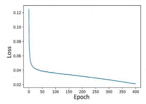
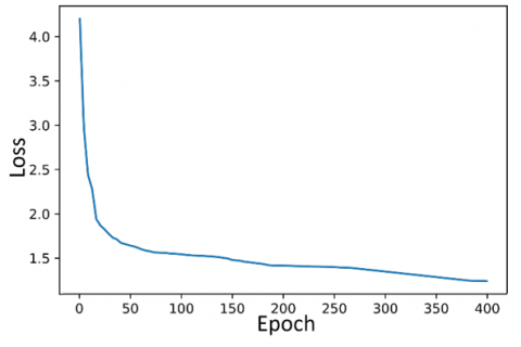
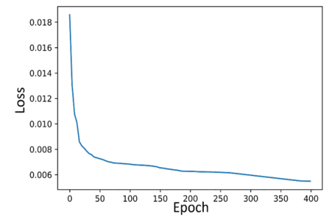
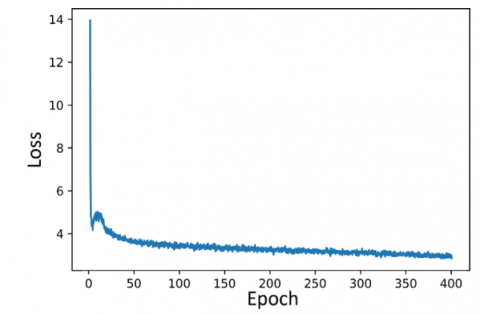
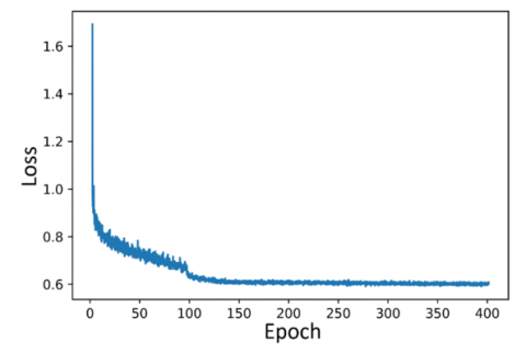
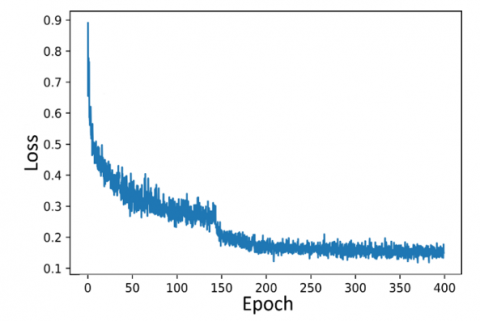
The training loss curves are shown in Figure 7, where the coordinates represent the epoch and loss values. The epoch number in this study was limited to 400. During the training process of a successful CNN model, the loss is expected to decrease gradually while accuracy increases progressively. Increasing the number of epochs can reduce fluctuations in the loss curve; however, this comes at the cost of extended training time. As illustrated in Figure 7, the loss curves of the models show a steep initial decline, which continues until a certain value is reached, after which the loss value stabilizes.
Among the loss graphs, the highest fluctuation at the end of 400 iterations is observed in the TOOD (ResNeXt101) model. The FCOS (ResNeXt101) and TOOD (ResNeXt101) models show a downward trend in loss until approximately 150 iterations, after which the loss value remains nearly constant. In contrast, the other models maintain their downward trend until the 400th iteration. However, this continued decrease is not substantial enough to significantly impact the results. At the end of training, YOLOv7 (E-ELAN-x) achieved the lowest loss value among all models, demonstrating its effectiveness in learning the features of the raisin images.
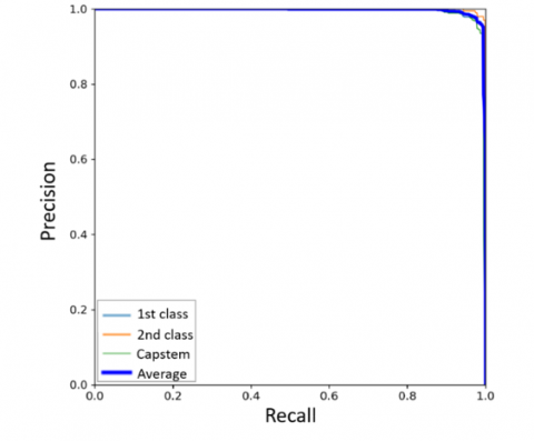
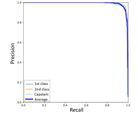
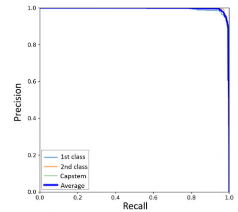
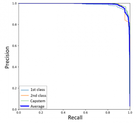
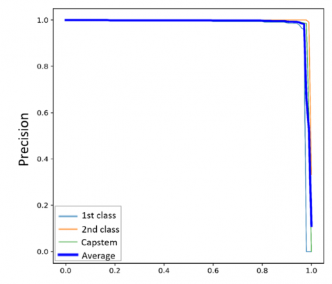
Precision-recall (P-R) curves illustrate the tradeoff between precision and recall as the model's threshold changes. To ensure all defects are detected, recall should be maximized; however, this often results in an increase in misclassified samples, thereby reducing precision. Ideally, the upper-right corner of the curve (where both recall and precision reach 100%) represents a perfect result [30]. The P-R curves of all models are shown in Figure 8, including curves for the 1st class, 2nd class, and capstem, as well as the average curve. For all models, the curves approach 100% on both the precision and recall axes. However, the P-R curve for the 2nd class in the YOLOX (CSPDarknet-x) model exhibits lower values compared to the others.
The models used in this study were compared based on different backbone networks, as presented in Table 2. The best results were achieved with an IoU threshold of 0.50. Across 14 different models, the mean mAP for IoU=0.50 was calculated as 98.8%. Among the models, the highest mAP value for IoU=0.50 was obtained with YOLOX (CSPDarknet-s), while the lowest mAP value was observed with FCOS (ResNetXt101). The 3.5% difference between the highest and lowest mAP values for IoU=0.50 indicates that the performance of the models is relatively consistent.
The size of the raisins and capstems detected in this study is most relevant to IoU=s. In experiments conducted with IoU=s, the mean mAP value was calculated as 76.4%. Among the models, the highest mAP value for IoU=s was achieved with FCOS (ResNet50), whereas the lowest mAP value was observed with YOLOv6 (EfficientRep-1).
To evaluate the robustness of the models without data augmentation, we conducted multiple training runs for each model-backbone combination using five different random seeds (42, 100, 2023, 7, 99). The mean mAP and standard deviation (±) values were calculated to assess the consistency of the models' performance across different initialization conditions. These values are reported in Table 2.
With data augmentation, multiple training runs were performed for each model-backbone combination using five random seeds (42, 100, 2023, 7, 99). The resulting mean mAP and standard deviation (±) values are presented in Table 3.
The experimental results presented in Table 2 (without data augmentation) and Table 3 (with data augmentation) demonstrate the significant impact of data augmentation techniques on model performance. Without data augmentation, the mean mAP (IoU=0.5) values were generally lower across all model-backbone combinations. For instance, YOLOv5 with the CSPDarknet-x backbone achieved a mean mAP of 90.1% without augmentation, compared to 99.1% with augmentation. Similarly, YOLOv7 with the E-ELAN-x backbone improved from 91.3% to 99.3% after applying data augmentation.
These results indicate that data augmentation techniques, including exposure adjustment, rotation, and noise addition, not only expanded the dataset size but also enhanced the diversity of training samples, enabling the models to generalize better. This improvement is particularly evident in challenging cases, such as small object detection (mAP IoU=s), where performance gains were more pronounced.
Sample results obtained from the best-performing model are presented in Figure 9.
(a) The loss curve of YOLOv5 (CSPDarknet-x)
(b) The loss curve of YOLOv6 (EfficientRep-l)
(c) The loss curve of YOLOv7 (E-ELAN-x)
(d) The loss curve of YOLOX (CSPDarknet-x)
(e) The loss curve of FCOS (ResNeXt10)
(f) The loss curve of TOOD (ResNeXt101)
Figure 7. The loss curves of all models
(a) The P-R curve of YOLOv5 (CSPDarknet-x)
(b) The P-R curve of YOLOv6 (EfficientRep-l)
(c)The P-R curve of YOLOv7 (E-ELAN-x)
(d) The P-R curve of YOLOX (CSPDarknet-x)
(e) The P-R curve of FCOS (ResNeXt10)
(f) The P-R curve of TOOD (ResNeXt101)
Figure 8. The P-R curve of the best models on the test set
Table 2. Performance comparison of state-of-the-art models without augmented data
|
Backbone |
MAP IoU=.50:.5:.95 |
MAP IoU=.50 |
MAP IoU=.75 |
MAP IoU=s |
MAP IoU=m |
MAP IoU=l |
Std(±) |
|
|
YOLOv5 |
CSPDarknet-s |
74.3 |
89.2 |
81.0 |
68.1 |
73.2 |
77.0 |
0.22 |
|
CSPDarknet-x |
78.4 |
90.1 |
83.7 |
70.5 |
74.8 |
79.1 |
0.25 |
|
|
YOLOv6 |
EfficientRep-s |
72.6 |
89.0 |
83.0 |
60.4 |
72.3 |
76.8 |
0.18 |
|
EfficientRep-l |
75.0 |
88.3 |
81.5 |
58.2 |
71.0 |
74.9 |
0.20 |
|
|
YOLOv7 |
E-ELAN-s |
76.2 |
91.5 |
83.0 |
65.3 |
70.5 |
77.4 |
0.15 |
|
E-ELAN-x |
78.8 |
91.3 |
84.5 |
68.7 |
73.1 |
79.5 |
0.17 |
|
|
YOLOX |
CSPDarknet-s |
75.2 |
92.3 |
84.0 |
69.2 |
72.9 |
77.3 |
0.19 |
|
CSPDarknet-x |
75.5 |
90.0 |
84.3 |
70.5 |
72.5 |
78.1 |
0.22 |
|
|
FCOS |
ResNet50 |
77.1 |
90.8 |
84.0 |
73.5 |
74.6 |
80.3 |
0.24 |
|
ResNet101 |
70.5 |
90.0 |
82.5 |
65.2 |
70.4 |
74.1 |
0.28 |
|
|
ResNeXt101 |
68.2 |
89.1 |
80.0 |
65.0 |
69.0 |
72.5 |
0.25 |
|
|
TOOD |
ResNet50 |
71.8 |
87.5 |
80.2 |
72.0 |
69.5 |
75.5 |
0.20 |
|
ResNet101 |
70.0 |
88.1 |
81.5 |
71.2 |
68.3 |
73.9 |
0.22 |
|
|
ResNeXt101 |
76.0 |
89.5 |
83.2 |
73.0 |
71.0 |
76.0 |
0.23 |
Table 3. Performance comparison of state-of-the-art models with augmented data
|
Backbone |
MAP IoU=.50:.5:.95 |
MAP IoU=.50 |
MAP IoU=.75 |
MAP IoU=s |
MAP IoU=m |
MAP IoU=l |
Std(±) |
|
|
YOLOv5 |
CSPDarknet-s |
84.6 |
99.0 |
92.1 |
78.2 |
81.2 |
84.3 |
0.15 |
|
CSPDarknet-x |
88.7 |
99.1 |
93.0 |
79.2 |
83.1 |
86.1 |
0.17 |
|
|
YOLOv6 |
EfficientRep-s |
82.6 |
99.1 |
93.9 |
67.3 |
82.1 |
85.0 |
0.12 |
|
EfficientRep-l |
84.1 |
98.3 |
91.3 |
63.5 |
79.2 |
84.6 |
0.14 |
|
|
YOLOv7 |
E-ELAN-s |
83.5 |
99.2 |
92.3 |
75.1 |
80.2 |
85.3 |
0.08 |
|
E-ELAN-x |
85.5 |
99.3 |
93.5 |
78.3 |
82.1 |
86.4 |
0.09 |
|
|
YOLOX |
CSPDarknet-s |
83.5 |
99.7 |
93.5 |
78.6 |
82.5 |
85.2 |
0.11 |
|
CSPDarknet-x |
83.7 |
99.1 |
93.6 |
82.1 |
82.9 |
87.5 |
0.14 |
|
|
FCOS |
ResNet50 |
85.8 |
99.0 |
94.0 |
84.6 |
85.1 |
89.1 |
0.16 |
|
ResNet101 |
82.3 |
99.2 |
92.4 |
72.1 |
80.1 |
82.2 |
0.19 |
|
|
ResNeXt101 |
79.8 |
96.2 |
90.8 |
73.2 |
80.2 |
82.8 |
0.15 |
|
|
TOOD |
ResNet50 |
82.8 |
98.0 |
91.3 |
79.7 |
80.8 |
86.3 |
0.09 |
|
ResNet101 |
80.1 |
98.9 |
93.0 |
78.2 |
80.3 |
83.2 |
0.12 |
|
|
ResNeXt101 |
85.1 |
99.1 |
94.3 |
79.6 |
82.3 |
85.1 |
0.17 |
Figure 9. Sample results of raisin images detected by the best model
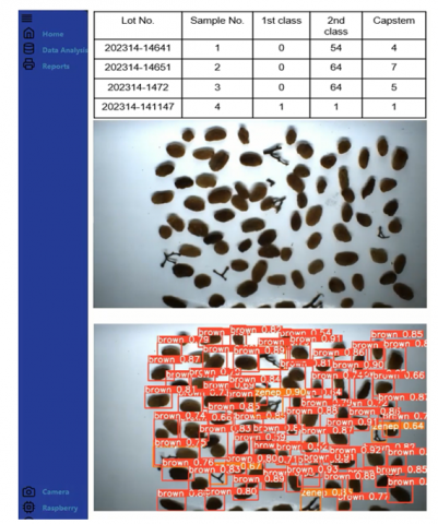
Figure 10. GUI for the developed system
The original image, the detected image, and the GUI software displaying database records are shown in Figure 10. For each 100-gram raisin sample, a record is created in the database, documenting the numbers of 1st class, 2nd class, and capstem raisins in the sample.
This study aims to classify raisins based on their color and the amount of capstem and non-herbal substances, in compliance with the TS 3411 seedless raisin standard. The current study has certain limitations that should be addressed in future work. One limitation is the manual placement of raisins on the conveyor belt in 100-gram samples, which may introduce variability in sample preparation and does not fully replicate automated industrial processes. Additionally, while the system successfully classifies raisins into three categories (1st class, 2nd class, and capstem), it lacks a physical mechanism to sort these categories in real-time, limiting its direct applicability in production lines. The camera height was optimized at 25cm to balance the field of view and image clarity; however, this fixed setup may not be suitable for different conveyor belt designs or raisin sizes. Furthermore, detecting smaller objects such as capstems in highly cluttered samples remains challenging, indicating a need for further refinement in training strategies and data augmentation techniques.
Future research could focus on addressing the limitations identified in the current study to enhance the system's applicability and performance. One potential direction is the integration of an automated feeding mechanism to replace manual sample placement, ensuring consistent and reproducible results. Additionally, incorporating a real-time sorting mechanism to physically separate raisins into categories would significantly improve the system's industrial usability. Expanding the dataset by including samples from diverse regions or other raisin varieties could further enhance the model's generalization capability. Furthermore, adapting the system to comply with other international standards or applying it to similar agricultural products would broaden its application scope. Finally, exploring advanced model architectures or improved data augmentation techniques could address challenges related to small object detection in cluttered environments, making the system more robust and effective.
In this study, foreign matter in Sultana-type raisins was identified according to the TS3411 quality standard, and quality classification was performed based on color. Additionally, a real-time system was developed to evaluate the suitability of raisin samples for export. A dataset comprising 2,636 raisin images was created, categorized into 1st class, 2nd class, and Capstem classes. Six different CNN models were trained using various backbone networks. The highest performance values were observed at IoU=0.50, with an overall mean mAP of 98.8% across all models.
The lighter color of certain raisins posed a challenge for the models, making detection more difficult. However, a notable outcome of the study is that all models accurately classified all 1st class raisins with a light yellow color, demonstrating their robustness in distinguishing this category.
[1] Food and Agriculture Organization of the United Nations & International Organisation of Vine and Wine. (2016). https://www.oiv.int/public/medias/5116/booklet-fao-oiv-grapes-focus.pdf, retrieved on April 21, 2025.
[2] ITC, List of exporters for the dried grapes in 2021. https://www.trademap.org/Country_SelProduct, accessed on May 1, 2023.
[3] Miran, B., Atiş, E., Bektaş, Z., Salalı, E., Cankurt, M. (2013). An analysis of ınternational raisin trade: A gravity model approach. In 57th AARES Annual Conference, Sydney, Australia, pp. 1-17. https://ageconsearch.umn.edu/record/152200/files/SP%20Miran.pdf.
[4] Turkish Standards Institute. (2014). Turkish seedless raisins grape standards. Ankara.
[5] Ramos, R.P., Gomes, J.S., Prates, R.M., Simas Filho, E.F., Teruel, B.J., dos Santos Costa, D. (2021). Non‐invasive setup for grape maturation classification using deep learning. Journal of The Science of Food and Agriculture, 101(5): 2042-2051. https://doi.org/10.1002/jsfa.10824
[6] Huang, Z., Wang, R., Zhou, Q., Teng, Y., Zheng, S., Liu, L., Wang, L. (2022). Fast location and segmentation of high‐throughput damaged soybean seeds with invertible neural networks. Journal of The Science of Food and Agriculture, 102(11): 4854-4865. https://doi.org/10.1002/jsfa.11848
[7] Uğuz, S., Uysal, N. (2021). Classification of olive leaf diseases using deep convolutional neural networks. Neural Computing and Applications, 33(9): 4133-4149. https://doi.org/10.1007/s00521-020-05235-5
[8] Lawal, O.M. (2021). YOLOMuskmelon: Quest for fruit detection speed and accuracy using deep learning. IEEE Access, 9: 15221-15227. https://doi.org/10.1109/ACCESS.2021.3053167
[9] Hussain, N., Farooque, A.A., Schumann, A.W., McKenzie-Gopsill, A., Esau, T., Abbas, F., Acharya, B., Zaman, Q. (2020). Design and development of a smart variable rate sprayer using deep learning. Remote Sensing, 12(24): 4091. https://doi.org/10.3390/rs12244091
[10] Zhang, J., Rao, Y., Man, C., Jiang, Z., Li, S. (2021). Identification of cucumber leaf diseases using deep learning and small sample size for agricultural Internet of Things. International Journal of Distributed Sensor Networks, 17(4): 15501477211007407. https://doi.org/10.1177/15501477211007407
[11] Tong, K., Wu, Y., Zhou, F. (2020). Recent advances in small object detection based on deep learning: A review. Image and Vision Computing, 97: 103910. https://doi.org/10.1016/j.imavis.2020.103910
[12] Mollazade, K., Omid, M., Arefi, A. (2012). Comparing data mining classifiers for grading raisins based on visual features. Computers and Electronics in Agriculture, 84: 124-131. https://doi.org/10.1016/j.compag.2012.03.004
[13] Yu, X., Liu, K., Wu, D., He, Y. (2012). Raisin quality classification using least squares support vector machine (LSSVM) based on combined color and texture features. Food and Bioprocess Technology, 5: 1552-1563. https://doi.org/10.1007/s11947-011-0531-9
[14] Çınar, İ., Koklu, M., Taşdemir, Ş. (2020). Classification of raisin grains using machine vision and artificial intelligence methods. Gazi Mühendislik Bilimleri Dergisi, 6(3): 200-209.
[15] Khojastehnazhand, M., Ramezani, H. (2020). Machine vision system for classification of bulk raisins using texture features. Journal of Food Engineering, 271: 109864. https://doi.org/10.1016/j.jfoodeng.2019.109864
[16] Zhao, Y., Guindo, M.L., Xu, X., Shi, X., Sun, M., He, Y. (2019). A novel raisin segmentation algorithm based on deep learning and morphological analysis. Engenharia Agrícola, 39: 639-648. https://doi.org/10.1590/1809-4430-Eng.Agric.v39n5p639-648/2019
[17] Roboflow Docs. https://roboflow.com, accessed on May 1, 2023.
[18] Arora, M., Mangipudi, P., Dutta, M.K. (2021). Deep learning neural networks for acrylamide identification in potato chips using transfer learning approach. Journal of Ambient Intelligence and Humanized Computing, 12(12): 10601-10614. https://doi.org/10.1007/s12652-020-02867-2
[19] Selvam, L., Kavitha, P. (2020). Classification of ladies finger plant leaf using deep learning. Journal of Ambient Intelligence and Humanized Computing, 11(11): 1-9. https://doi.org/10.1007/s12652-020-02671-y
[20] Simonyan, K., Zisserman, A. (2014). Very deep convolutional networks for large-Scale image recognition. arXiv Preprint arXiv: 1409.1556. https://doi.org/10.48550/arXiv.1409.1556
[21] Fuentes, A.F., Yoon, S., Lee, J., Park, D.S. (2018). High-performance deep neural network-Based tomato plant diseases and pests diagnosis system with refinement filter bank. Frontiers in Plant Science, 9: 1162. https://doi.org/10.3389/fpls.2018.01162
[22] Xiong, Y., Liang, L., Wang, L., She, J., Wu, M. (2020). Identification of cash crop diseases using automatic image segmentation algorithm and deep learning with expanded dataset. Computers and Electronics in Agriculture, 177: 105712. https://doi.org/10.1016/j.compag.2020.105712
[23] Ismail, N., Malik, O.A. (2022). Real-Time visual inspection system for grading fruits using computer vision and deep learning techniques. Information Processing in Agriculture, 9(1): 24-37. https://doi.org/10.1016/j.inpa.2021.01.005
[24] LeCun, Y., Bottou, L., Bengio, Y., Haffner, P. (1998). Gradient-Based learning applied to document recognition. Proceedings of the IEEE, 86(11): 2278-2324. https://doi.org/10.1109/5.726791
[25] Krizhevsky, A., Sutskever, I., Hinton, G.E. (2017). ImageNet classification with deep convolutional neural networks. Communications of the ACM, 60(6): 84-90. https://doi.org/10.1145/3065386
[26] Zheng, H., Wang, G., Li, X. (2022). YOLOX-Dense-CT: A detection algorithm for cherry tomatoes based on YOLOX and DenseNet. Journal of Food Measurement and Characterization, 16(6): 4788-4799. https://doi.org/10.1007/s11694-022-01553-5
[27] de Aguiar, A.S.P., dos Santos, F.B.N., dos Santos, L.C.F., de Jesus Filipe, V.M., de Sousa, A.J.M. (2020). Vineyard trunk detection using deep learning-An experimental device benchmark. Computers and Electronics in Agriculture, 175: 105535. https://doi.org/10.1016/j.compag.2020.105535
[28] Li, Y., Li, M., Qi, J., Zhou, D., Zou, Z., Liu, K. (2021). Detection of typical obstacles in orchards based on deep convolutional neural network. Computers and Electronics in Agriculture, 181: 105932. https://doi.org/105932. 0.1016/j.compag.2021.105932
[29] Uğuz, S. (2020). Automatic olive peacock spot disease recognition system development by using single shot detector. Sakarya University Journal of Computer and Information Sciences, 3(3): 158-168. http://doi.org/10.35377/saucis.03.03.755269
[30] Da Costa, A.Z., Figueroa, H.E., Fracarolli, J.A. (2020). Computer vision based detection of external defects on tomatoes using deep learning. Biosystems Engineering, 190: 131-144. https://doi.org/10.1016/j.biosystemseng.2019.12.003