Lei Yan![]() | Gang Liu*
| Gang Liu*![]() | Chenle Yu
| Chenle Yu![]()
© 2025 The authors. This article is published by IIETA and is licensed under the CC BY 4.0 license (http://creativecommons.org/licenses/by/4.0/).
OPEN ACCESS
With the continuous advancement of remote sensing technology, the application of remote sensing images in fields such as environmental monitoring and urban planning has been significantly expanded. Accurate classification of remote sensing images is essential for effective image analysis and interpretation. However, traditional supervised classification methods rely heavily on large volumes of labeled data, which are often costly and difficult to obtain in practical scenarios. To address this challenge, unsupervised remote sensing image classification has attracted increasing research interest. Recently, the introduction of Generative Adversarial Networks (GANs) and transfer learning has provided new strategies and technical pathways for unsupervised classification tasks. GANs enhance feature representation by generating images that closely resemble the original data, while transfer learning enables existing knowledge to be leveraged for improved classification performance in target tasks. Although notable progress has been achieved, existing unsupervised classification methods still face considerable challenges. Traditional unsupervised learning approaches often exhibit low classification accuracy under complex environmental conditions, particularly in feature extraction and noise resistance. While deep learning-based methods have improved classification performance to some extent, their effectiveness remains limited by factors such as training data volume and network architecture design. Therefore, enhancing the classification accuracy and robustness of remote sensing images by combining the strengths of GANs and transfer learning remains a critical research problem. In this study, an unsupervised remote sensing image classification method based on GANs and transfer learning was proposed. Initially, remote sensing images were augmented using GANs to generate richer feature representations, thereby improving the effectiveness of subsequent classification. Subsequently, an unsupervised classification method that incorporates transfer learning was introduced, enabling the utilization of existing model knowledge to further enhance classification accuracy. Experimental results demonstrate that the proposed method achieved superior classification accuracy and robustness in remote sensing image classification tasks, offering a promising new direction for the development of unsupervised remote sensing image classification techniques.
remote sensing images, unsupervised classification, Generative Adversarial Networks (GANs), transfer learning, image enhancement, classification accuracy
With the rapid development of remote sensing technology, the application of remote sensing images has been significantly expanded across various fields, including environmental monitoring, urban planning, and agricultural management [1-4]. The classification of remote sensing images is considered a critical component of remote sensing image processing [5, 6]. Traditional supervised classification methods typically rely on large volumes of labeled data; however, the labeling process is labor-intensive and incurs high costs [7, 8]. In practical applications, the difficulty of obtaining large-scale annotated datasets has driven the growing research interest in unsupervised remote sensing image classification, establishing it as a significant direction in the field of remote sensing image analysis.
Unsupervised learning methods have enabled the learning of features from data autonomously, thereby avoiding the complexities associated with manual annotation and offering greater flexibility in addressing large-scale data processing challenges [9, 10]. In particular, the introduction of GANs and transfer learning has substantially promoted the application of unsupervised learning in remote sensing image classification. GANs have made it possible to enhance remote sensing images effectively by generating realistic images without the need for labeled data, thereby improving feature representation capabilities [11, 12]. Transfer learning has further facilitated the application of existing knowledge and models to achieve improved classification performance on target tasks [13]. These technologies have created new opportunities and posed new challenges for the classification of remote sensing images.
Despite the significant progress achieved by existing unsupervised learning-based remote sensing image classification methods, several limitations remain. Many approaches continue to encounter challenges in terms of classification accuracy and the effectiveness of feature extraction [9, 14, 15], particularly under complex environmental conditions, where the diversity and complexity of images hinder further improvements in classification performance. For example, the unsupervised method based on feature learning proposed by Li et al. [16] often relies on manually designed features, rendering it ineffective in adapting to the varied backgrounds and noise present in remote sensing images. Although the unsupervised method based on deep learning described by Suryawati et al. [17] enables end-to-end learning through neural networks, its performance remains constrained by the volume of training data and the limitations of network architecture, making it difficult to address small-sample problems effectively. Furthermore, how to combine the advantages of GANs and transfer learning to further enhance classification accuracy and image enhancement remains an open and critical challenge in current research.
In this study, an unsupervised remote sensing image classification approach based on the integration of GANs and transfer learning was proposed. First, to address the challenge of preliminary image enhancement, an unsupervised remote sensing image enhancement method based on GANs was introduced, capable of generating clearer and richer feature representations to provide improved data support for subsequent classification tasks. Subsequently, an unsupervised classification method combining GANs and transfer learning was proposed, in which the knowledge of existing models is transferred to strengthen the classification network's performance, and GANs were further employed to optimize the classification results. Experimental validation demonstrates that the proposed method achieved superior performance in both classification accuracy and robustness for remote sensing image classification tasks. This research not only provides a novel perspective for remote sensing image classification technology but also lays a foundation for the future development of advanced remote sensing image processing techniques.
2.1 Assessing the importance of samples in model training
Remote sensing images are typically characterized by complex spectral features, varying spatial resolutions, and significant background variations. During the training process, certain regions or classes of samples may dominate, potentially leading to model bias toward specific categories. Analyzing the importance of samples to the model training process is therefore crucial for identifying those samples that contribute significantly to the learning of the classifier, as well as those that exert minimal influence or introduce noise.
To quantify the influence of each sample during training, the contribution of individual samples to the neural network's loss function must be evaluated. Given the high dimensionality and the complex spatial and spectral information inherent in remote sensing images, some samples may exhibit strong feature representations during training, while others may have limited impact due to the presence of noise, blurring, or low-quality regions. In order to assess sample importance more precisely, a Model Correlation Index (MCI) was introduced. Samples with high MCI values are generally those that contain distinctive and highly discriminative features, effectively reflecting the differences among various land cover categories in remote sensing imagery.
Specifically, the training sample set is denoted as T={(au,bu)}2u=1, where the neural network output in the form of a probability vector is represented by o(q,a), the weights at the s-th iteration are denoted by Qs, and the loss function is indicated by loss(.). The gradient of the loss function with respect to the weights is represented by hs(a,b). The variation of the loss function with training iterations can thus be expressed as follows:
$\begin{aligned} & \Delta_s((a, b), T)=-\frac{d}{d s} \operatorname{loss}\left(o\left(q_s, a\right), b\right) \\ & \approx-\frac{d \operatorname{loss}\left(o\left(q_s, a\right), b\right)}{d q_s} \cdot\left(q_{s+1}-q_s\right) \\ & =\frac{d \operatorname{loss}\left(o\left(q_s, a\right), b\right)}{d q_s} \cdot \lambda \sum_{(a, b) \in T} h_s(a, b)\end{aligned}$ (1)
If any sample (ak,bk) is removed from T, the contribution of the training sample set to the variation in the loss function can be expressed as:
$\begin{aligned} & \left\|\Delta_s((a, b), T)-\Delta_s\left((a, b), T_{-k}\right)\right\| \\ & =\left\|\lambda \frac{d \text { loss }}{d q_s} \sum_{(a, b) \in T} h_s(a, b)-\lambda \frac{d \text { loss' }}{d q_s} \sum_{(a, b) \in T_{-k}} h_s(a, b)\right\| \\ & \leq \lambda\left\|\frac{d \text { loss }}{d q_s}\right\| \cdot\left\|h_s\left(a_k, b_k\right)\right\|=z\left\|h_s\left(a_k, b_k\right)\right\|\end{aligned}$ (2)
Assuming that the expected value of the gradient norm is denoted by Rqs||hs(a,b)||2, and substituting this into the activation function and error formulation of the neural network, the MCI can be represented as follows:
$M C I=R\left\|o\left(q_s, a\right)-b\right\|_2$ (3)
MCI characterizes the influence of each sample on the parameter updates during the model training process. To facilitate a unified evaluation, the MCI values were normalized into a range of [0 100] for statistical analysis. The specific transformation formula is given by:
$M C I^{D F}=\frac{U_{L U}-M I N\left(U_{L U}\right)}{M A X\left(U_{L U}\right)-\operatorname{MIN}\left(U_{L U}\right)}$ (4)
2.2 Assessing the correlation between samples and the classification boundary
In remote sensing image classification, the classification boundary is typically defined by decision boundaries in a high-dimensional feature space. In unsupervised learning, the absence of labeled data often results in unclear classification boundaries, making it difficult to accurately separate different image regions. Therefore, assessing the correlation between each sample and the classification boundary is critical for identifying samples located near the classification boundary.
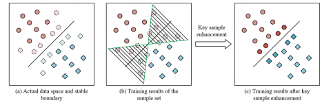
Figure 1. Illustration of samples and the classification boundary
Figure 1 illustrates the relationship between samples and the classification boundary. As shown in the figure, samples situated close to the boundary generally exert a significant influence on classifier training, as they represent regions with the highest uncertainty in classification decisions. The accuracy of the classifier is highly sensitive to these samples. By enhancing the representation of these boundary samples or applying appropriate weighting during training, the classification capability of the model near boundary regions can be substantially improved, thereby enhancing overall classification performance. Specifically, a Boundary Correlation Index (BCI) was introduced to describe the relationship between each sample and the classification boundary. Let the system's classification decision criteria be denoted by |UST|, then the following formulation is given:
$B C I=L N\left(\frac{1}{\left|U_{S T}\right|^{0.5}+0.5}\right)+\frac{1}{\left|U_{S T}\right|^2+0.5}$ (5)
For consistency in evaluation, the BCI values were normalized into the [0 100] range for statistical analysis. The specific transformation formula is provided as follows:
$B C I^{D F}=\frac{U_{Y Z}-\operatorname{MIN}\left(U_{Y Z}\right)}{\operatorname{MAX}\left(U_{Y Z}\right)-\operatorname{MIN}\left(U_{Y Z}\right)}$ (6)
2.3 Sample importance index (SII)
The calculation of the SII enables the contribution of each sample to classifier training to be quantified, allowing for a more precise identification of samples that exert a significant influence on the model. For instance, certain typical samples in remote sensing images, such as specific land cover types, may possess distinctive spectral or morphological features that render them highly important during training. In contrast, noisy or atypical samples may exert minimal impact on the learning process. By computing the SII, the model is capable of identifying the most representative and most challenging samples, thereby focusing on enhancing the learning of these samples.
Based on the preceding analysis, it can be observed that the numerical distributions of the MCI and the BCI differ, particularly in regions near the classification boundary and the physical boundary. To comprehensively assess the contribution of samples to model training, an SII was defined by integrating information from both MCI and BCI. Specifically, MCI reflects the impact of a sample on the loss function, highlighting samples that significantly influence model learning, while BCI emphasizes the proximity of a sample to the actual physical boundary. Especially in remote sensing images, land cover boundaries are often key areas in classification. By combining MCI and BCI, SII enables the identification of key samples that are both highly relevant to the model and located near physical boundaries, thus providing a prioritized basis for image enhancement. The specific calculation formula is given by:
$S I I^{D F}=\left\{\begin{array}{l}\frac{M C I^{D F}+B C I^{D F}}{2}, M C I^{D F} \geq 50 \\ M C I^{D F}, M C I^{D F}<50\end{array}\right.$ (7)
2.4 Key sample enhancement based on GANs
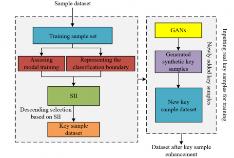
The fundamental principle of preliminary unsupervised remote sensing image enhancement based on GANs is to generate additional synthetic samples that closely resemble the features of key samples, thereby expanding the training dataset and particularly enhancing those samples with high importance indices. The overall process is illustrated in Figure 2. In unsupervised remote sensing image classification, certain land cover boundary regions often exhibit ambiguous features, making it difficult for the training process to adequately learn and distinguish these areas. The generator within the GANs continuously learns from real samples to produce synthetic samples that closely approximate the original images in terms of detail, texture, and structure. These synthetic samples enrich the diversity of the training data provided to the model. The discriminator is responsible for distinguishing between real and generated samples and, through adversarial learning with the generator, promotes the continuous optimization of the generator to produce increasingly realistic outputs. This dynamic adversarial process enables the generator to produce remote sensing images that closely resemble real data, particularly in regions with complex boundaries or ambiguous features, thereby supplying more accurate and representative samples for subsequent classification tasks. Specifically, let the discriminator be denoted by F, the generator by H, the real sample data distribution by ODA, and the noise data distribution by oNO, with the noise data serving as input to the generator H. The objective function of the GANs can thus be expressed as:
$M I N_H M I N_F R_{x \sim O_{D A}}\binom{\log (F(a))}{+R_{x \sim O_{N O}} \log (1-H(c))}$ (8)
Figure 2. Flowchart of the key sample enhancement scheme based on GANs
3.1 Model architecture
In the proposed unsupervised remote sensing image classification model integrating GANs and transfer learning, the GAN module comprises a feature generator and a feature discriminator. The generator learns from real remote sensing images to produce synthetic images with similar attributes, while the discriminator is tasked with distinguishing between generated and real images. Through adversarial training, the generator is continuously optimized to produce increasingly realistic remote sensing images. During this process, the feature generator not only creates images beneficial for classification but also enhances complex land cover boundaries or transition zones within remote sensing images, particularly in regions that are ambiguous or difficult to identify. A general feature extractor and a specific feature extractor, based on the Visual Geometry Group (VGG)16 model, are responsible for in-depth feature extraction from target domain images. The general feature extractor captures basic features such as texture and shape, whereas the specific feature extractor focuses on detailed features within remote sensing images, including land cover types and boundary information.
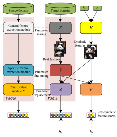
The introduction of the transfer learning module, particularly the knowledge transfer between the source and target domains, constitutes a core component of the model. The source domain utilizes a large-scale image dataset to pre-train the VGG16 model, during which the general feature extraction module, specific feature extraction module, and classification module undergo preliminary training. The task in the source domain involves learning a classification function from the source domain samples to provide foundational knowledge support for the target domain. In the target domain, transfer learning enables the model to fine-tune itself by leveraging the knowledge acquired from the source domain, thereby improving classification performance. During learning in the target domain, the feature extractor and classifier of the VGG16 model integrate the generated image features and transferred knowledge to facilitate the identification of land cover types within remote sensing images. Particularly in the unsupervised learning setting, where target domain remote sensing images typically lack labels, the transfer learning module plays a critical role by effectively transferring deep features learned from the source domain to the target domain, thereby enhancing the classifier's recognition capability. The model architecture is shown in Figure 3.
Figure 3. Architecture of the unsupervised remote sensing image classification model combining GANs and transfer learning
In the unsupervised remote sensing image classification model, the primary objective of the feature generator is to produce high-quality synthetic feature maps for evaluation by the feature discriminator. The inputs to the feature generator include random noise sampled from a uniform distribution and one-hot encoded class labels. The random noise introduces diversity, ensuring sufficient variability in the generated features, while the one-hot encoding provides category-specific information to guide the generation of discriminative synthetic samples across different classes. These inputs are concatenated and passed through a fully connected layer and a reshaping layer to generate 512 small feature maps of size 4×4. These small feature maps pass through a series of transposed convolutional layers, batch normalization layers, and activation layers, gradually increasing in spatial size while reducing the number of channels, eventually producing feature maps of size 64×64 with 128 channels. For unsupervised remote sensing images, this generator design enables the learning of not only basic textures and shapes but also complex land cover boundaries and transitional features. Particularly in regions with ambiguous or difficult-to-classify land features, the generator enhances the representation, providing richer training samples for subsequent classification tasks.
The feature discriminator is designed to distinguish whether the input feature maps were generated by the feature generator or extracted from real remote sensing images. Its input consists of tensors with a size of 64×64 and 128 channels, identical to the output of the feature generator. The discriminator is responsible for extracting semantic information from the feature maps through convolutional layers, batch normalization layers, and activation layers, followed by fully connected layers that output a scalar as the discrimination score. This score represents the discriminator's judgment on whether the input features are true features. A higher score indicates a greater likelihood that the input features are real, while a lower score suggests that the features are more likely to have been generated. In the context of unsupervised remote sensing image classification, where land cover boundaries and transitional zones are often blurred and difficult to distinguish, the discriminator is progressively optimized during training to enhance its sensitivity to these complex regions, thereby encouraging the generator to produce more refined land cover boundary features.
The general feature extractor is designed to extract fundamental features from the input real remote sensing images to assist in classification tasks. This extractor employs the first half of the VGG16 network architecture, consisting of four convolutional layers and corresponding max pooling layers, to extract low-level features such as textures, edges, and shapes from 256×256 three-channel color images. Given that remote sensing images typically contain abundant land cover information and complex background noise, the general feature extractor not only captures the basic structural characteristics of land objects but also assists the model in identifying regional differences and boundaries between different land cover types. By extracting these low-level features, the model can provide inputs with higher discriminative potential for the subsequent specific feature extractor, facilitating the further extraction of classification-relevant features. Ultimately, the output of the general feature extractor is feature maps of size 64×64 with 128 channels, which are used for subsequent feature processing and classification tasks.
The specific feature extractor is designed to extract higher-level features that are more classification-focused from the real features generated by the general feature extractor or the synthetic features produced by the GAN. This module inherits the latter half of the VGG16 architecture, comprising nine convolutional layers and corresponding max-pooling layers, and processes the lower-level features through deeper feature extraction. The input to the specific feature extractor consists of feature maps of size 64×64 with 128 channels, which are progressively processed to reduce the spatial dimensions to 8×8 while increasing the number of channels to 512. This design enables the specific feature extractor to deeply mine complex details in remote sensing images, such as the textural features of specific land cover types, inter-object relationships, and boundary features. In unsupervised remote sensing image classification, the specific feature extractor must not only process geometric and textural information but also address regions that are difficult to classify due to noise or occlusion, thereby providing high-quality inputs for subsequent classification tasks.
The feature classifier is responsible for classifying the high-level semantic features extracted by the specific feature extractor. Within the unsupervised learning framework, the role of the feature classifier is to recognize the categories of remote sensing images and accomplish land cover classification. The classifier adopts the classification module of the VGG16 model, which includes the final three fully connected layers, with appropriate parameter adjustments to ensure compatibility with remote sensing image features. Specifically, the number of neurons in the final fully connected layer is set to match the number of classes in the dataset, and activation is performed using a softmax function to output the probability distribution over the classes. In the context of unsupervised remote sensing images, the feature classifier determines the category of an image based on the deep semantic features obtained from the specific feature extractor. Given the complexity of land cover types and the broad spatial distribution often observed in remote sensing images, the classifier must possess strong discriminative capabilities to distinguish subtle land cover differences and accurately classify images from the target domain. By combining the features learned from the source domain with the specific features of the target domain, the feature classifier effectively performs land cover classification in the absence of labels, ultimately achieving the objective of unsupervised remote sensing image classification.
In the proposed unsupervised remote sensing image classification model, the structures of the target domain general feature extractor, target domain specific feature extractor, and target domain feature classifier are identical to those of the general feature extractor, specific feature extractor, and feature classifier of the overall model. However, differences exist in the sources of their parameters and their training approaches. The target domain general feature extractor adopts parameters from the pre-trained VGG16 model on the source domain through parameter sharing. This allows the target domain general feature extractor to leverage the feature extraction capabilities learned from the source domain, thereby facilitating rapid adaptation to the feature characteristics of remote sensing images in the target domain. Through this approach, the target domain general feature extractor can effectively extract low-level features such as textures, shapes, and boundary information from target domain remote sensing images, providing a solid foundation for subsequent classification tasks. In contrast, the general feature extractor of the model is trained from scratch without loading the pre-trained parameters from the source domain, which may result in the learning of more basic features in the target domain and a lack of utilization of source domain prior knowledge. Moreover, differences also exist in the training of the parameters for the target domain specific feature extractor and the target domain feature classifier. The target domain specific feature extractor obtains its parameters through fine-tuning based on the pre-trained VGG16 model from the source domain. This fine-tuning enables slight adjustments to the source domain model to better fit the feature characteristics of the target domain remote sensing images. Through fine-tuning, the target domain specific feature extractor can capture more task-relevant features, particularly those related to complex land cover boundaries, transitional zones, and detailed land cover types in remote sensing images. In contrast, the specific feature extractor of the model is entirely trained from scratch, without utilizing any pre-trained information from the source domain, which may lead to lower efficiency in feature extraction, especially when the amount of target domain data is limited. The target domain feature classifier acquires its parameters through parameter replacement, based on the VGG16 model pre-trained on the source domain. This means that the classification capability trained on the source domain can be directly adopted, with only the parameters of the final fully connected layer replaced to adapt to the class labels of the target domain. By comparison, the model’s feature classifier does not utilize pre-trained parameters from the source domain and therefore relies entirely on learning from the target domain data. This reliance may impose greater challenges on the training process and classification accuracy under unsupervised learning conditions.
In the model, the source domain general feature extraction module, source domain specific feature extraction module, and source domain classification module are designed to fully leverage the pre-trained parameters from the source domain to enhance the feature extraction and classification capabilities of the target domain model. The source domain general feature extraction module shares the same structure as the target domain general feature extractor, both adopting the first half of the VGG16 model, which includes four convolutional layers and corresponding max-pooling layers. Through parameter sharing, the pre-trained network parameters from the source domain are directly copied into the target domain general feature extractor, and these parameters are kept frozen during training. This design ensures that the target domain general feature extractor can fully utilize the low-level feature extraction capabilities learned from the large-scale labeled dataset of the source domain, thereby effectively extracting basic features such as textures, edges, and shapes from target domain remote sensing images. Similarly, the source domain specific feature extraction module shares an identical structure with the target domain specific feature extractor, both based on the latter half of the VGG16 model, which consists of nine convolutional layers and corresponding max-pooling layers. However, unlike the general feature extraction module, the specific feature extraction module adopts a fine-tuning-based transfer learning strategy. The network parameters of the source domain specific feature extraction module are copied to the target domain specific feature extractor, and these parameters are allowed to be updated during training on the target domain. Through this approach, the specific feature extractor can be further adjusted and optimized based on the pre-trained parameters, better adapting to the feature characteristics of target domain remote sensing images. Additionally, although the source domain classification module and the target domain feature classifier differ structurally, the latter can use the classification capability of the source domain model through parameter replacement. By replacing the parameters of the final fully connected layer, the target domain feature classifier can be adapted to the classification tasks of the small-scale dataset in the target domain.
3.2 Loss function
In the model, the design principle of the feature generator follows that of a classical GAN, with the core objective of generating realistic synthetic features that deceive the feature discriminator, thereby promoting the learning of more discriminative and representative features for remote sensing images. Specifically, the input to the feature generator consists of a noise vector c sampled from a uniform distribution Oc and a class label bc. These inputs are transformed by the feature generator H into synthetic feature vectors. To achieve the objective of making the feature discriminator F unable to distinguish between real and synthetic features during training, a negative log-likelihood loss was employed for the feature generator’s loss function. This encourages the generation of increasingly realistic synthetic features such that the feature discriminator assigns high scores to them, as if they were extracted from real remote sensing images. The loss function for the feature generator is expressed as:
$M_H=-R_{c \sim O_e}\left[F\left(H\left(c, b_z\right)\right)\right]$ (9)
The design of the feature discriminator's loss function aims to distinguish between real features extracted from remote sensing images and synthetic features generated by the feature generator, thereby driving the generation of more realistic and high-quality features. The feature discriminator's goal is to correctly classify the authenticity of the input features by assigning high scores to real features and low scores to synthetic ones. The loss function for the feature discriminator consists of three components. The first term, structurally similar to the feature generator’s loss function, uses a negative log-likelihood formulation to maximize the ability to distinguish real from synthetic features during training. Given the high diversity in land cover types, textures, shapes, and spectral characteristics in remote sensing images, the feature discriminator must effectively capture these complex feature differences to successfully distinguish between real and synthetic features. The second and third terms of the loss function correspond to the classification of real image samples and the application of a gradient penalty, respectively. In the second term, A represents real image samples drawn from the real data distribution ODA. The negative sign indicates that the feature discriminator should assign higher scores to real features during training, thereby strengthening its ability to recognize features from real remote sensing images. This component enhances the model's understanding of target domain features, particularly under unsupervised learning conditions, where it enables effective learning of critical feature information from remote sensing images. The third term introduces a gradient penalty coefficient, designed to constrain the gradient of the discriminator with respect to the input features, ensuring that the gradient norm is close to one. This mechanism is intended to prevent issues such as gradient vanishing or explosion, which may lead to instability during the training process of GANs, affecting the model’s convergence.
$\begin{aligned} & M_F=R_{c \sim O_z}\left[F\left(H\left(c, b_z\right)\right)\right]-R_{a \sim o_{D, A}}[F(E(a))] \\ & +\eta R_{\dot{d} \sim o_d}\left[\left(\left\|\nabla_{\dot{d}} D(\dot{d})\right\|_2-1\right)^2\right]\end{aligned}$ (10)
In the model, the design principle of the target domain feature classifier is to accurately predict the category of the input remote sensing image, thereby achieving efficient classification. The loss function for the target domain feature classifier is based on the cross-entropy loss, aiming to minimize the discrepancy between the predicted and actual categories. Specifically, the input to the target domain feature classifier consists of the specific features d extracted by the target domain specific feature extractor. These features are classified by the feature classifier Z, and the cross-entropy loss is computed between the predictions and the true labels. The cross-entropy loss function MZ effectively measures the divergence between the predicted probability distribution and the actual class distribution, thereby guiding the model to adjust its parameters during training and improve classification accuracy. Due to the complex and diverse information contained in remote sensing images, such as varying land cover types, intricate textures, and spectral features, the classification model is required to possess strong feature extraction and discrimination capabilities. By employing the cross-entropy loss, the target domain feature classifier is continuously optimized during training to better capture these complex features and accurately classify remote sensing images into their respective categories. Assuming that the loss function of the target domain specific feature extractor is denoted by Mt, and the loss function of the target domain feature classifier is denoted by MZ, it leads to the following expression:
$M_T=M_Z=R_{a \sim O_{D d}}\left[-b_z \log Z(T(d))\right]$ (11)
In the model, a second loss function for the feature generator is designed not only to ensure that the generated synthetic features are realistic enough to confuse the feature discriminator but also to guarantee that these synthetic features can be correctly classified by the target domain feature classifier. The core objective of this design is to align the category information of synthetic features with that of real features, thereby minimizing the category discrepancy between synthetic and real features. The second loss function of the feature generator, MH2, is optimized by concatenating real features and synthetic features. Specifically, after concatenation, the combined features are input into the target domain feature classifier to compute the classification results, and the cross-entropy loss between the classifier’s output and the true labels is computed. Assuming that the concatenated features are denoted as d⌒ and the mathematical expectation is represented by R, it leads to the following expression:
$M_{H 2}=R\left[-b_z \log Z(T(\hat{d}))\right]$ (12)
The feature generator provides additional training data for the target domain specific feature extractor and the feature classifier by generating realistic synthetic features. These synthetic features are concatenated with real features to form new training samples. The second loss function of the target domain specific feature extractor comprises three components: the first focuses on the classification loss for synthetic features, the second addresses the classification loss for real features, and the third concerns the predicted classification loss for concatenated features. The combination of these three losses ensures that the target domain specific feature extractor is capable not only of extracting features from real images but also of effectively handling generated synthetic features. As a result, the feature extractor becomes more robust and is able to accurately extract target domain-specific features even under interference from various types of image features. In the context of unsupervised remote sensing image classification, such a data augmentation mechanism is particularly critical, as remote sensing images often contain complex textures, shapes, and spectral information. Introducing synthetic features into the training process significantly enhances the model's ability to learn these complex characteristics. The second loss function of the target domain feature classifier is closely tied to that of the loss function of the target domain specific feature extractor, with the aim of strengthening the classification ability by incorporating synthetic features.
Specifically, the target domain feature classifier evaluates the classification results for synthetic features, real features, and concatenated features, computing the cross-entropy loss between the predicted outputs and the true class labels. The design principle behind these three losses is to ensure that the classifier can effectively distinguish among different feature categories, particularly under unsupervised learning conditions. By introducing synthetic features, the classifier’s discrimination ability for specific categories is enhanced. Furthermore, weight coefficients are assigned to the three losses to balance their contributions, adjusting the impact of real features, synthetic features, and concatenated features during classifier training. This design not only strengthens the target domain feature classifier’s ability to learn remote sensing image categories but also mitigates the potential negative effects of synthetic features on classification results, ensuring high classification accuracy even in a mixed environment of real and synthetic data. Ultimately, through the optimization of the loss functions for the target domain specific feature extractor and feature classifier, improved classification performance and generalization capability are achieved in the unsupervised remote sensing image classification task. Assuming that the concatenation of synthetic and real features is denoted by d⌒, the real features by d, the synthetic features by d*, and the feature concatenation operation by ⊕, and that the corresponding loss weights are represented by ε1, ε2, and ε3, the second loss functions of the target domain specific feature extractor and the target domain feature classifier, denoted by MT2 and MZ2, are formulated as:
$\begin{aligned} & M_{T 2}=M_{Z 2}=\varepsilon_1 R_{c \sim o_e}\left[-b_z \log Z\left(T\left(H\left(c, b_z\right)\right)\right)\right] \\ & +\varepsilon_2 R_{a \sim o_{\Delta d}}\left[-b_z \log Z(T(E(a)))\right] \\ & +\varepsilon_3 R_{d \sim d}\left[-b_z \log Z(T(\hat{d}))\right]\end{aligned}$ (13)
3.3 Training process
The training process for the unsupervised remote sensing image classification model, which integrates GANs and transfer learning, is designed to progressively enhance the classification performance on the target domain through the alternating training of the feature generator, feature discriminator, target domain specific feature extractor, and target domain feature classifier, particularly under conditions where labeled data are scarce. The training process comprises multiple stages, each aimed at optimizing the relationship between the generated synthetic features and the real features, while ensuring that the final model can accurately classify different types of remote sensing images. At the beginning of training, the network parameters of the feature generator and feature discriminator were initialized. Subsequently, by applying transfer learning, the weights of the source domain general feature extraction module were transferred to the target domain general feature extractor, and the weights of the source domain specific feature extraction module were transferred to the target domain specific feature extractor. In the initial phase, the feature generator was tasked with producing synthetic features, while the target domain general feature extractor extracted real features from target domain images. The feature discriminator was then trained using both real and synthetic features to enable it to distinguish between them during training. Initially, the feature discriminator possessed only limited discriminative capability; however, through continuous training and optimization, its ability to distinguish real from synthetic features was gradually improved.
As training progresses, the weights of the feature discriminator were fixed, and the subsequent stage focused on training the feature generator to produce increasingly realistic synthetic features. During this stage, the feature generator was optimized to learn how to generate synthetic features from random noise inputs that are sufficiently realistic to pass the feature discriminator’s judgment. Meanwhile, the target domain general feature extractor continued to extract real features, and the target domain specific feature extractor and target domain feature classifier were trained to ensure correct classification of the extracted real features.
Subsequently, the focus of training was shifted toward further improving the feature generator. After fixing the weights of the target domain feature classifier, the feature generator was required not only to produce realistic synthetic features but also to ensure that these synthetic features conform to the category distribution of the target domain. Through joint training with real features, synthetic features, and corresponding category labels, the feature generator was gradually optimized to produce synthetic data that match the characteristic attributes of the target classes.
In the later stages of training, the parameters of the feature generator were periodically fixed after a certain number of iterations. The synthetic features generated by the feature generator, together with the real features extracted by the target domain general feature extractor, were then used to train the target domain specific feature extractor and the target domain feature classifier. The objective of this stage is to ensure that the target domain specific feature extractor and classifier are capable not only of correctly classifying real features but also of accurately handling synthetic features. This process enhances the robustness and classification accuracy of the classifier. By continuously repeating these training steps, the model progressively improved classification accuracy in the unsupervised remote sensing image classification task, ultimately achieving efficient and accurate classification performance even in the absence of labeled data.
As shown in Table 1, the classification results on the test set demonstrate that, for the vegetation class, the baseline VGG16 achieved an accuracy of 0.7652, which was improved to 0.7785 after geometric augmentation. VGG16-Transformer achieved 0.8125, and VGG16+Squeeze-and-Excitation (SE) further increased performance to 0.9632. The proposed model achieved the highest performance at 0.9751. For the water body class, the baseline VGG16 and the geometrically augmented VGG16 both achieved 0.4236, while VGG16-Transformer improved to 0.4426. VGG16+SE showed a substantial improvement to 0.7541, and the proposed model achieved the best result of 0.8562. In the artificial surface class, the baseline VGG16 achieved 0.1236, which slightly decreased to 0.1126 after geometric augmentation. VGG16-Transformer improved to 0.1625, and VGG16+SE reached 0.3326. The proposed model significantly outperformed all others, achieving 0.4236. It can be observed that the proposed model attained the best performance across all three land cover classes, while the other improved models also achieved varying degrees of enhancement compared to the baseline. The experimental results demonstrate that the unsupervised remote sensing image classification method, which combines GAN-based image enhancement with transfer learning, is highly effective. The GAN-based image enhancement method provided higher-quality training data for classification. The classification method integrating transfer learning with GANs enhanced the network’s representational capability through knowledge transfer, and the results were optimized through GANs. This enabled the proposed model to outperform all comparative models in the classification of vegetation, water bodies, and artificial surfaces. Although VGG16+SE demonstrated the beneficial effect of feature enhancement, the proposed model, by leveraging both the data augmentation advantages of GANs and the knowledge transfer capabilities of transfer learning, achieved superior classification performance, validating the effectiveness and advancement of the proposed approach in unsupervised remote sensing image classification.
Table 1. Summary of unsupervised remote sensing image classification results on the test set
|
VGG16 Dataset |
Baseline VGG16 |
Geometric Augmentation VGG16 |
VGG16-Transformer |
VGG16+SE |
Proposed Model |
|
Vegetation class |
0.7652 |
0.7785 |
0.8125 |
0.9632 |
0.9751 |
|
Water body class |
0.4236 |
0.4236 |
0.4426 |
0.7541 |
0.8562 |
|
Artificial surface class |
0.1236 |
0.1126 |
0.1625 |
0.3326 |
0.4236 |
As shown in the curves of Figure 4, the training set loss (blue line) for the vegetation and water body classes exhibited a clear decreasing trend with an increasing number of training epochs, while the test set loss (red line), although fluctuating, also showed an overall gradual decline. For the artificial surface class, the training set loss decreased rapidly during the early stages, and the test set loss, after a brief decline, tended to stabilize. These observations indicate that, as training progressed, the model’s fitting capability for the classification tasks across vegetation, water body, and artificial surface classes was continuously enhanced, and a certain degree of generalization ability was also demonstrated on the test data. Despite fluctuations during training, the overall trend in loss function values reflected continuous optimization. The results suggest that the proposed unsupervised remote sensing image enhancement method based on GANs effectively provided higher-quality data for the classification tasks, enabling the model to learn features more efficiently during training. The continuous decrease in training set loss demonstrated the model’s adaptability to the enhanced data. Furthermore, the integration of transfer learning with GANs optimized the classification network. As reflected in the test set loss trends, under unsupervised conditions, the model was able to gradually enhance classification performance across different land cover classes by leveraging both transferred knowledge and the optimization capabilities of GANs.
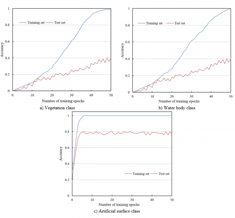
Figure 5 presents the variation in classification accuracy of unsupervised remote sensing image samples with respect to training epochs. For the vegetation and water body classes, the training set accuracy (blue line) continuously increased with additional training, rising from near zero to nearly one. Although the test set accuracy (red line) exhibited fluctuations, an overall upward trend was observed. For the artificial surface class, the training set accuracy rose rapidly during the early stages, while the test set accuracy experienced a significant initial improvement and then remained relatively stable, fluctuating between 0.6 and 0.8. These results indicate that, as the number of training epochs increased, the model's fitting capability on the training data was progressively enhanced, while a certain degree of generalization ability was also demonstrated on the test data. Despite the presence of fluctuations, the overall classification accuracy exhibited a positive optimization trend. Experimental results confirm that the unsupervised remote sensing image enhancement method based on GANs provided a high-quality data foundation for the classification tasks, enabling the model to effectively learn land cover features. The continuous rise in training set accuracy reflected the model’s strong adaptability to the enhanced data. In addition, the integration of transfer learning with GANs optimized the classification network. As indicated by the trends in test set accuracy, under unsupervised conditions, the model was able to gradually improve classification performance across different land cover classes by leveraging transferred knowledge and the optimization capabilities of GANs.
Figure 4. Variation curves of the unsupervised remote sensing image classification loss function with respect to training epochs
Figure 5. Variation curves of classification accuracy for unsupervised remote sensing image samples with respect to training epochs
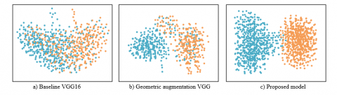
Figure 6. t-SNE visualization of feature distributions of unsupervised remote sensing images on the test set
Figure 6 presents the t-distributed Stochastic Neighbor Embedding (t-SNE) visualization results of unsupervised remote sensing image feature distributions on the test set. In the feature distribution of the baseline VGG16, the blue and orange points are highly intermixed, indicating low inter-class separability. Although the features of the geometric augmentation VGG exhibit partial separation, significant overlap remains. In contrast, the proposed model demonstrates highly compact clusters of blue and orange points, with minimal overlap, reflecting excellent class separability in the feature space. These results indicate that the proposed model possesses superior feature learning capabilities, effectively distinguishing between different categories. It can be concluded that the proposed model provides clearer and more enriched image features, and that the newly developed unsupervised classification method—combining transfer learning with GANs—further optimizes both the feature extraction and the classification network. The high degree of feature separability achieved by the proposed model in low-dimensional space validates its ability to significantly enhance feature discriminability, leading to improved classification performance.
This study primarily focused on the development and implementation of an unsupervised remote sensing image classification method by integrating GANs and transfer learning techniques. The core objective was to address the challenges inherent in unsupervised remote sensing image classification, particularly in scenarios with limited labeled data, by enhancing feature representation and classification performance through the combination of two advanced deep learning approaches—GANs and transfer learning. This research holds significant theoretical and practical value. Theoretically, it provides a novel approach for unsupervised remote sensing image classification by leveraging GANs and transfer learning to overcome data scarcity and improve the model's learning capacity. From an application perspective, the proposed method is of great significance for the automated classification of remote sensing images, particularly in fields such as disaster monitoring, land cover change analysis, and environmental protection, where improvements in classification accuracy and efficiency are crucial. By integrating GANs with transfer learning, an innovative solution was presented in this study that substantially addresses the limitations of traditional unsupervised remote sensing image classification methods in terms of feature extraction and classification accuracy.
However, despite the achievements attained in this study, several limitations remain. First, the training process of the GAN model may suffer from instability, particularly in the generation of synthetic features, where issues such as mode collapse may arise, adversely affecting the diversity and quality of generated images. Second, although transfer learning significantly enhances the performance of the classification network, the selection of an appropriate source domain model to ensure the effectiveness of transfer learning remains an open question requiring further investigation. Moreover, the proposed model was primarily optimized for remote sensing image data, and its generalizability and adaptability to other image classification tasks have yet to be validated. Future research directions could be pursued along the following lines: First, the training stability and generative quality of GANs could be further optimized, particularly through the design of more efficient adversarial frameworks to mitigate mode collapse. Second, the selection of source domain models warrants deeper exploration to achieve stronger domain adaptation during transfer learning, thereby enhancing classification accuracy on target domain data. Additionally, future studies could explore the integration of multi-modal remote sensing data, combining different data types such as optical images and radar images, to improve model diversity and applicability. Through these advancements, future unsupervised remote sensing image classification methods are expected to achieve improved performance and broader applicability in real-world scenarios.
[1] Andrés, S., Arvor, D., Mougenot, I., Libourel, T., Durieux, L. (2017). Ontology-based classification of remote sensing images using spectral rules. Computers & Geosciences, 102: 158-166. https://doi.org/10.1016/j.cageo.2017.02.018
[2] Ding, X.Y., Hu, W.J., Hu, G.B., Liu, F. (2023). Mineral element identification in remote sensing imagery: A fusion approach using CH-Tucker decomposition and RFDNet. Traitement du Signal, 40(4): 1501-1509. https://doi.org/10.18280/ts.400418
[3] Zhang, Q., Zhang, J., Lu, S., Liu, Y., Liu, L., Wang, Y.Y., Cao, M.Y. (2023). Multi-resolution feature extraction and fusion for traditional village landscape analysis in remote sensing imagery. Traitement du Signal, 40(3): 1259-1266. https://doi.org/10.18280/ts.400344
[4] Ullah, S.U., Zeb, M., Ahmad, A., Ullah, S., Khan, F., Islam, A. (2024). Monitoring the billion trees afforestation project in Khyber Pakhtunkhwa, Pakistan Through Remote Sensing. Acadlore Transactions on Geosciences, 3(2): 89-97. https://doi.org/10.56578/atg030203
[5] Kumar, D.G., Chaudhari, S. (2024). Auxg: Deep feature extraction and classification of remote sensing image scene using attention unet and xgboost. Journal of the Indian Society of Remote Sensing, 52(8): 1687-1698. https://doi.org/10.1007/s12524-024-01908-z
[6] Gu, Y., Wang, Y., Li, Y. (2019). A survey on deep learning-driven remote sensing image scene understanding: Scene classification, scene retrieval and scene-guided object detection. Applied Sciences, 9(10): 2110. https://doi.org/10.3390/app9102110
[7] Agnelli, D., Bollini, A., Lombardi, L. (2002). Image classification: an evolutionary approach. Pattern Recognition Letters, 23(1-3): 303-309. https://doi.org/10.1016/S0167-8655(01)00128-3
[8] Ke, B., Lu, H., You, C., Zhu, W., Xie, L., Yao, Y. (2024). A semi-supervised medical image classification method based on combined pseudo-labeling and distance metric consistency. Multimedia Tools and Applications, 83(11): 33313-33331. https://doi.org/10.1007/s11042-023-16383-w
[9] Madadi, Y., Seydi, V., Nasrollahi, K., Hosseini, R., Moeslund, T.B. (2020). Deep visual unsupervised domain adaptation for classification tasks: A survey. IET Image Processing, 14(14): 3283-3299. https://doi.org/10.1049/iet-ipr.2020.0087
[10] Eckhardt, C.M., Madjarova, S.J., Williams, R.J., Ollivier, M., Karlsson, J., Pareek, A., Nwachukwu, B.U. (2023). Unsupervised machine learning methods and emerging applications in healthcare. Knee Surgery, Sports Traumatology, Arthroscopy, 31(2): 376-381. https://doi.org/10.1007/s00167-022-07233-7
[11] Fadaeddini, A., Majidi, B., Souri, A., Eshghi, M. (2023). Data augmentation using fast converging CIELAB-GAN for efficient deep learning dataset generation. International Journal of Computational Science and Engineering, 26(4): 459-469. https://doi.org/10.1504/IJCSE.2023.132152
[12] Crino, N., Cox, B.A., Gaw, N.B. (2024). Garbage In≠ Garbage Out: Exploring GAN resilience to image training set degradations. Expert Systems with Applications, 250: 123902. https://doi.org/10.1016/j.eswa.2024.123902
[13] Herath, S., Fernando, B., Harandi, M. (2019). Using temporal information for recognizing actions from still images. Pattern Recognition, 96: 106989. https://doi.org/10.1016/j.patcog.2019.106989
[14] Sandoval, C., Pirogova, E., Lech, M. (2021). Adversarial learning approach to unsupervised labeling of fine art paintings. IEEE Access, 9: 81969-81985. https://doi.org/10.1109/ACCESS.2021.3086476
[15] Slavkovikj, V., Verstockt, S., De Neve, W., Van Hoecke, S., Van de Walle, R. (2016). Unsupervised spectral sub-feature learning for hyperspectral image classification. International Journal of Remote Sensing, 37(2): 309-326. https://doi.org/10.1080/01431161.2015.1125554
[16] Li, T., Qian, Y., Li, F., Liang, X., Zhan, Z. H. (2024). Feature subspace learning-based binary differential evolution algorithm for unsupervised feature selection. IEEE Transactions on Big Data, 11(1): 99-114. https://doi.org/10.1109/TBDATA.2024.3378090
[17] Suryawati, E., Pardede, H.F., Zilvan, V., Ramdan, A., Krisnandi, D., Heryana, A., Supianto, A.A. (2021). Unsupervised feature learning-based encoder and adversarial networks. Journal of Big Data, 8: 1-17. https://doi.org/10.1186/s40537-021-00508-9