Radhakrishnan Kuppusamy*![]() | Leena Jasmine John Sundarabai
| Leena Jasmine John Sundarabai![]()
© 2025 The authors. This article is published by IIETA and is licensed under the CC BY 4.0 license (http://creativecommons.org/licenses/by/4.0/).
OPEN ACCESS
Automated computer-assisted tools based on deep learning explored promising results in the instant and accurate prediction of Brain cancers. However, the availability of large medical imaging datasets for training deep-learning models remains limited. In this work, a hybrid approach for brain tumor classification using a Generative Adversarial Network (GAN) called DenseUnetGAN is proposed. The GAN-based model incorporates pre-trained models in the generator and discriminator components. Specifically, a modified U-Net architecture serves as the generator, while DenseNet is utilized as the discriminator and classifier after modifying the fully connected layers. Further, the hyperparameters of the GAN model are tuned using Lemur’s optimizer. By leveraging pre-trained models and the GAN framework, the proposed approach is presented to enhance the efficiency and accuracy of brain tumor classification despite the limitations of limited data availability. Through extensive experimentation and evaluation, it demonstrates the effectiveness among brain tumor classes. The results highlight the potential of the proposed model for improving the diagnosis of brain tumors, thereby aiding healthcare professionals and reducing the burden on healthcare systems.
deep learning, GAN, U-Net, disease diagnosis, classification, learning models
An abnormal cells enlargement within the brain is known as tumor. Brain tumors encompass a wide range of neoplasms in the human body, which exhibit diverse characteristics influenced by factors including the cell of origin, location, structure, and manner of progression [1].
The tumor is divided into primary and secondary tumors. Approximately 60% of all brain tumors are primary tumors, while the remaining 40% are classified as secondary tumors. The classification is based on the source of the tumors, where primary tumors initiate in the brain itself. Conversely, secondary tumors initiate in remaining body parts and later spread to the brain. It is important to mention that the majority of secondary tumors, around 40%, are malignant [2].
Medical image analysis has undergone a transformative advancement in practicality and innovative approaches, primarily driven by rapid hardware development and the utilization of sophisticated mathematical tools. These advancements enable the acquisition of highly detailed medical images [3, 4]. Leveraging these medical images, accurate and efficient image analysis techniques can assist healthcare professionals in diagnosing and treating patients effectively.
An imaging method is available for the segmentation and classification of brain tumors, among which MRI is utilized as a non-invasive approach. The popularity of MRI stems from its advantages, such as ionizing radiation absence, greater resolution of soft tissues, and the capability to capture various images through different imaging parameters. There has been significant research interest in the development of automated AI-based intelligent systems. Presently, various automated systems are provided using Machine Learning (ML), transfer learning approaches, and Deep Learning (DL) models [5]. Traditional approaches to classifying brain tumors using ML algorithms involve multiple steps, such as feature extraction and classification. Feature extraction and selection pose requires domain expertise, precision of classification relies on the identification of relevant features.
GANs are a type of DL model that consists of a Generator (G) and a Discriminator (D) network [6]. GANs have been employed in various medical imaging tasks, including image synthesis, image-to-image translation, data augmentation, and anomaly detection. A key difference between traditional generative models and GANs is that GANs learn the distribution of the input as a complete image rather than making pixels individually. The proposed work is contributed as follows:
•Proposing the new U-Net architecture model for the generator part of the GAN model classification using automated MRI image processing.
•Proposing the new GAN model for rapid tumor classification using automated MRI images.
•The classification task of the model is improved by applying Lemur’s optimization for parameter tuning.
•The constructed GAN model is compared with the other models.
The remaining sections of the work are as follows: Section 2 presents the related works of existing literature, Section 3 introduces the DenseUnetGAN model, Section 4 describes the results and discussion, and finally, Section 5 concludes the paper.
This section reviews several related works that employ DL techniques to detect and classify brain tumours. Vidyarthi et al. [7] proposed a novel Cumulative Variance method-based feature selection for brain MRI. The extracted features are used to train different ML models like AdaBoost, neural networks and decision trees. Among these, the neural network shows higher classification accuracy.
In their work, Yu et al. [8] proposed an improved sparrow search approach to classify brain tumor. The search strategy of the sparrow is applied to select relevant training features. The optimum feature selection increases the model's classification accuracy by 4.5% compared to without optimization.
Yang et al. [9] proposed a tumor segmentation based on Dual Disentanglement Network (D2-Net) that employs a spatial frequency to decouple modality-specific data from a dataset, which enables segmentation even with missing modalities.
Sultan et al. [10] explored a convolutional neural network (CNN) for tumor detection. The developed model is applied in two datasets to classify with an overall accuracy of 95.45% and 97.6%.
Another CNN model was developed by Huang et al. [11] based on complex networks to categorize brain tumors. The network structure is created using randomly generated graph algorithms, eliminating the need for manual design and optimization. The CNN model based on complex networks achieves an accuracy of 95.49%, outstanding other models in previous work.
Asif et al. [12] utilized popular DL architectures, including Xception, GoogleNet, DenseNet121, and ResNet, for brain tumor diagnosis. Pre-trained models are employed to extract deep features.
Shah et al. [13] proposed a DL based on the EfficientNet-B0 model to detect brain tumor efficiently. Data augmentation methods are improved the quality and increase the training data. The overall accuracy for classification and detection reaches 98.87%. Rizwan et al. [14] proposed a Gaussian CNN model with two datasets are utilized, one for classifying tumors and the other for distinguishing between three grades of glioma.
Imtiaz et al. [15] proposed a superpixel-level from 3D volumetric MR images. The images are partitioned into superpixels to capture precise boundaries. By considering image planes separately, the statistical and textural features are extracted from each superpixel. A feature selection scheme is introduced to reduce dimensionality while maintaining classification performance.
Zhou et al. [16] investigated UNet++ for tumor segmentation. UNet++ addresses an unknown network depth issue by using an ensemble of U-Nets with varying depths. It introduces redesigned skip connections to combine features from distinctive semantic scales, resulting in effective feature selection. Additionally, a pruning method is devised to accelerate inference speed without significant performance degradation. Likewise, Micallef et al. [17] developed a U-Net++ model for brain tumor segmentation. This modified model incorporates changes in the loss function and functional layers to increase network performance.
Alhassan and Zainon [18] proposed an automated segmentation method for brain tumor detection in MRI images. The approach utilizes pre-processing and segmentation processes, incorporating a modern learning-based method with the Bat Algorithm and Fuzzy C-ordered means clustering technique. Bat algorithms are employed to segment the tumor by calculating initial centroids and distances between pixels, distinguishing the tumor Region of Interest from non-tumor.
Gumaei et al. [19] proposed hybrid feature extraction, and extreme learning classification. Experimental results demonstrate improved accuracy compared to existing approaches, with accuracy increasing from 91.51% to 94.233%. Ferdous et al. [20] introduced linear-complexity data-efficient image transformers. Teacher-student methods are used to achieve high precision rates.
Noreen et al. [21] proposed a method for quick identification of brain tumors using multi-level feature learning and concatenation. Inception-v3 and DensNet201 DL models are employed for brain tumor detection and classification, achieving high testing accuracies of 93.9% and 94.24% respectively and demonstrating superior performance. Mishra et al. [22] introduced a self-supervised-based contrastive loss for feature learning. Unlabeled data is utilized to train a DL model through contrastive learning, maximizing similarity and contrastive instances learning. It outperforms random or ImageNet initialization for the classification of MRI images. Afshar et al. [23] introduced a modified CapsNet architecture by incorporating tumor coarse boundaries as extra inputs. This enhancement allows CapsNet to focus on the tumor while considering the surrounding tissues, improving its performance. The proposed approach significantly outperforms other methods, addressing the sensitivity of CapsNets to miscellaneous image backgrounds.
Mirza and Osindero [24] introduced a conditional version of generative adversarial networks (CGAN) for generating MNIST digits conditioned on class labels. The functioning of the GAN model can be varied based on the condition given by the user. Gurumurthy et al. [25] presented a GAN model for varied and limited training data environments. By reparameterizing the latent generative space and learning its parameters alongside the GAN, DeLiGAN enables variety in generated samples despite being trained with limited data.
Ghassemi et al. [26] presented a GAN method for tumor classification in MR images. By replacing the fully connected layers and training the network as a classifier, the proposed approach achieves effective tumor classification. Ge et al. [27] addressed brain tumor subcategory classification using MRI images from various imaging systems. To overcome limited datasets and incomplete modality issues, they employ a pairwise GAN model to generate synthetic MRIs across different modalities. A post-processing approach combining slice-level classification results is proposed, and a multi-stage training technique using GAN-augmented MRIs followed by real MRIs is employed.
Yerukalareddy and Pavlovskiy [28] proposed a DL model for brain tumor classification on MRI images. The trained DL model with an auxiliary classifier in a discriminator allows feature extraction and tumor classification. The model is tested on publicly available MRI datasets, achieving accurate classification of different brain tumor types.
Ahmad et al. [29] proposed a variational auto-encoder-based GAN named VAE-GAN. The developed GAN model uses an auto encoder to generate a noise pattern for the generator instead of generating random noise.
Chauhan et al. [30] proposed a modified DenseNet model for brain tumour detection with an accuracy of 95.68%. Milletari et al. [31] introduced a deep V-net network optimized by an improved Genetic optimization algorithm. The optimized V-net achieves 96.64% accuracy in medical image classification. In Huang’s research, the 3D U²-Net, which combines U-Net with an optimized classifier, achieved an accuracy of 95% [32]. Cheng et al. [33] applied transfer learning with ResNet50V2. It shows 94.68% accuracy for the public MRI dataset. Ejiyi et al. [34] developed a segmentation network with SegNet for tumor grade classification.
Based on the existing models for brain tumor classification face challenges with limited annotated datasets and poor generalization across diverse MRI images. Many approaches are based on manual hyperparameter tuning, which is time-consuming and inefficient. Additionally, synthetic data generated by conventional GANs often lacks the diversity and quality needed to improve model performance. These limitations highlight the need for a hybrid approach that uses pre-trained architectures with GANs to increase classification accuracy and robustness.
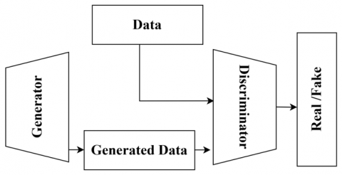
The GAN model has main elements like the Generator (G) and the Discriminator (D) [35]. The element ‘G’ is responsible for producing an output image that closely matches the distribution of the original image. The discriminator, depicted in Figure 1, is responsible for differentiating the generated image from the images generated by the generator model.
Figure 1. General GAN model [6]
While training, the generative model processes synthetic data, attempting to failure the process of discriminator by making the generated samples appear realistic. Simultaneously, the discriminator is trained to correctly classify whether a given sample is real or generated. As training progresses, the generative model increases its ability to produce more accurate outputs, while the discriminator becomes more talent to find the differ among real and generated data.
The proposed DenseUnetGAN model combines the strengths of DenseNet and U-Net architectures. Compared to traditional U-Net models, the propsoed model based on simple skip connections. The DenseUnetGAN integrates DenseNet's dense blocks to learn more complex feature representations by promoting feature reuse. The dense connection capture both local and global information more effectively. Additionally, the DenseUnetGAN incorporates a U-Net-based generator which is designed for precise image segmentation. The DenseNet discriminator helps to evaluate the realism of generated images by capturing intricate patterns across different scales.
3.1 DenseUnetGAN
In this work, the DenseUnetGAN model incorporates pre-trained models in the generator and discriminator components. Specifically, a modified U-Net architecture serves as the generator, while DenseNet is utilized as the discriminator and classifier after modifying the fully connected layers. In conventional GAN, the model tries to provide new images from random noise. The generator of the GAN has very few dimensions in input, but the output is of large dimensions.
In the proposed model, the modified UNet is the generator to generate fake images instead of generating from random noise. The proposed architecture with DenseUnetGAN model is given in Figure 2(a) and Figure 2(b).
The loss functions for the modified U-Net generator and DenseNet discriminator can be adjusted accordingly.
GAN Loss: The GAN objective function measures the adversarial loss among the generator and discriminator. It consists of two terms:
LGAN(G, D) = E(x, y) [log(D(x, y))] + E(x) [log(1 - D(x, G(x)))] (1)
G represents the modified U-Net generator, D represents the DenseNet discriminator, x is an input image, and y is the corresponding brain tumor category label Eq. (1). The first term aims to maximize the discriminator (x, y) as real, while the second term aims to maximize the discriminator data x and its corresponding generated data G(x) as fake.
Generator Loss: It used to process generator features to deceive discriminator. It is described in Eq. (2):
LGenerator(G, D) = λGAN * LGAN(G, D) (2)
where, λGAN is a hyperparameter that controls the importance of the GAN loss, and LGAN(G, D) is the GAN loss.
Discriminator Loss: It is used to distinguish real and fake data which has two classification losses:
LDiscriminator(G, D) = LClass(D, x, y) + LClass(D, x, G(x)) (3)
In Eq. (3) LClass(D, x, y) is the classification loss for the DenseNet discriminator applied to real data x with the corresponding ground truth label y. LClass(D, x, G(x)) is the classification loss for the discriminator applied to x and G(x).
Generator Classification Loss: In addition to the GAN loss, it includes a classification loss for the generator to directly optimize the classification task. It can be described in formal terms as follows Eq. (4):
LGenerator_Class(G, D) = LClass(G(x), y) (4)
where, LClass(G(x), y) is the classification loss for the DenseNet discriminator applied to the created data G(x) with the ground truth label y.
U-Nets have performed an efficient segmentation for a complex image. It consists of an encoder that gradually downsamples the input, learning the global context and a decoder that executes advanced upsampling to equal the output resolution with the input by allowing exact localization.
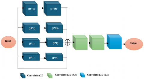
However, conventional U-Nets lack contextual information sharing between shallow and deep layers. To address this limitation and enhance the local and global features of the network, the modified U-Net architecture is introduced that is given in Figure 2(b). The Data Degradation Control Block with Contextual Aggregation (DDCBWCA) block is connected between the encoder to decoder is shown in Figure 3.
Figure 3. DDCBWCA block
The improved U-Net takes MRI input images and outputs images of the same dimensions. Convolution layers with padding are employed to ensure that the output image size matches the input size. The encoder side has convolution layers, pooling layers, and dropout layers to perform downsampling. On the decoder side, the output of DDCBWCA is connected to the Conv2DTranspose layer for feature control from the previous block. Finally, the dropout is applied to the concatenated output.
The Data Degradation Control Block with Contextual Aggregation plays a crucial role. It generates middle-level features, ensuring control over important degradation of features. The complex size variations issues of brain tumor size can be effectively handled by concatenated connections. The DDCBWCA connection makes the model scale invariant and allows contextual aggregation on multiple scales. The DDCBWCA expands the valid field to learn and improve its performance effectively.
The DDCBWCA block consists of five parallel connections, each processing the input data differently as shown in Figure 3. The first four connections apply two convolutional layers with a specific filter size: N×1 for the first convolution and 1×N for the second convolution. This approach decreases the number of parameters compared to N × N convolution layer. The impact of the cascaded convolution layers with fewer parameters is found to be similar to a single layer with more parameters.
Next, skip connection is used to preserve the original input. The outputs of all parallel connections are merged to obtain a single output. Then, three consecutive convolutional layers with filter sizes of 3×3, 3×3, and 1×1 are applied to the summed output.
The improved U-Net architecture incorporates the DDCBWCA module to bridge the gap between shallow and deep layers, enabling enhanced integration of local and global features. The DDCBWCA block uses dense connectivity combined with attention mechanisms to allow the network to focus on important features. Unlike standard UNet skip connections that directly concatenate encoder features with the decoder, this block provides better integration of local features and global features. It is used for better segmentation in complex tasks.
The discriminator in the DenseUnetGAN model is based on a DenseNet structure which includes several dense blocks stacked with multiple convolutional layers. Typically, the DenseNet discriminator consists of 4 to 5 layers of dense blocks with total feature maps growing from 64 in the initial layers to 512 in the deeper layers. This design enables the discriminator to attain both local and global features within the generated images. By focusing on a rich combination of feature patterns at multiple scales, the DenseNet discriminator significantly improves to differentiate among fake and real images.
3.3 Lemur optimizer based parameter tuning
Optimization is a crucial process used to provide the most favorable solution for a given problem while considering constraints. The objective function is typically minimized or maximized to determine the optimal outcome. Optimization plays a vital role in decision-making across various domains [36]. However, many real-world problems are intricate, involving multiple nonlinear constraints. This complexity adds to the difficulty of achieving effective optimization.
It is based on a metaheuristic optimization algorithm that is inspired by the behaviors of lemurs [37]. The two important behaviors of lemurs like leap-up and dance-hub. are statistically translated into solving optimization problems. In the exploration stage, the dance-hup behavior is used. Similarly, the leap-up behaviour is used for exploiting the search space. The problem solving approach is mathematically modelled as follows.
The solution for decision variable j with i as Eq. (5):
$S_i^j=r *\left(u l_j-l l_j\right) \forall i \in(1,2, \ldots . d)$ (5)
where, r is the random variable varies between zero to one.
$\begin{gathered}S_i^j= \left\{\begin{array}{l}s(i, j)+a b s(s(i, j)-s(B, j)) *(r-0.5) * 2 ; r<f_r \\ s(i, j)+a b s(s(i, j)-s(G, j)) *(r-0.5) * 2 ; r>f_r\end{array}\right.\end{gathered}$ (6)
where, B represents the nearest best lemur and G denotes global best lemur.
$f_r=f_r *(h r r)- curriter *(h r r-l r r) / maxiter$ (7)
where, $f_r$ is the free risk rate, hrr and lrr is high and low risk rates, curriter is the current iterations. The above steps are applied to the fitness function iteratively to get optimal GAN parameters. The pseudocode for proposed parameter tuning is given below:
Pseudocode: Lemur Optimizer based Tuning
1. Initialize parameters:
a. Initialize n lemurs (solutions) randomly within the bounds [ll, ul].
b. Set the current iteration to 0 (currIter = 0).
c. Define high-risk rate (hr) and low-risk rate ().
d. Evaluate the fitness of each lemur using F.
2. Determine the best lemur:
a. Identify the global best solution (G) with the highest fitness.
b. Identify the nearest best lemur (B) for each lemur based on fitness.
3. Loop until maxIter is reached:
a. For each lemur (i):
i. Generate a random number r in the range [0, 1].
ii. Update decision variable $S_i^j$ for each dimension j using Eq. (6).
b. Update $S_i^j$ using the Eq. (7).
c. Clip $S_i^j$ within bounds [ll, ul] to ensure valid solutions.
d. Evaluate the new fitness of each lemur using F.
e. Update the global best (G) and nearest best (B) lemurs based on the new fitness values.
4. Increment the iteration (currIter = currIter + 1).
5. Output the global best solution (G) as the optimal GAN parameters.
The algorithm starts by defining the population size, bounds, and other parameters. Each lemur's position represents a possible set of GAN parameters. The fitness function F evaluates how well the parameters perform in training the DenseUnetGAN model. In the early iterations, the algorithm prioritizes exploration, broadly searching across the parameter space. This is controlled by $f_r$, which starts high (encouraging risk-taking) and gradually decreases over time. As iterations progress, $f_r$ lowers, focusing on refining solutions near the best candidates. Lemurs move closer to either the closest best solution. The updated solutions are clipped to remain within the specified bounds. The process is repeated, adjusting positions and fitness evaluations, until the maximum number of iterations is reached. The global best solution (G) represents the optimal parameters for training DenseUnetGAN.
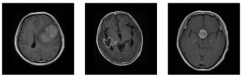
This work uses two datasets for the purpose of training and evaluating a classification method using MRI. The first dataset, created by Cheng et al. [38] comprises a total of 3064 T1-CE MR images. This dataset includes three distinct types of brain tumors: 708 meningioma tumors, 1426 glioma tumors, and 930 pituitary tumors. It encompasses MR images captured in all different planes. Table 1 offers simulation parameters related to this research study.
Table 1. Experimental settings
|
Parameter |
Value |
|
Dataset |
Brain Tumor Dataset (e.g., BRATS 2018) |
|
Train-Test Split |
80% train, 20% test |
|
Image Dimensions |
240×240×4 |
|
Batch Size |
16 |
|
Number of Epochs |
50 |
|
Optimizer |
Adam |
|
Learning Rate |
1e-4 |
|
Momentum |
0.9 |
|
Weight Decay |
1e-5 |
|
Data Augmentation |
Random rotations (10-30 degrees), flipping, scaling (0.8-1.2), elastic deformation |
|
Dropout Rate |
0.5 |
|
Activation Function |
ReLU and SoftMax |
|
Evaluation Metrics |
Dice Similarity Coefficient (DSC), IoU, Accuracy |
|
Hardware |
NVIDIA Tesla V100 (16GB VRAM) |
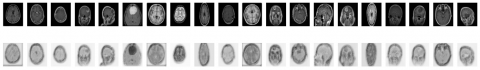
The second data set used in this study is a collection of whole brain volume MR images initially presented by Marcus et al. [39]. This dataset was primarily designed to investigate dementia in elders. It comprises longitudinal images of 372 sets obtained from 100 aged subjects among 50 and 93 years. The sample data set image is shown in Figure 4.
Figure 4. Data set image
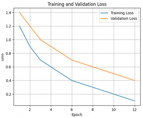
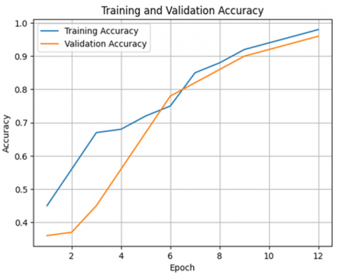
The DenseUnetGAN’s hyperparameters are tuned before evaluation. The best hyperparameters of the model are identified by lemur optimization. The fitness function is used to find the best values of the optimizer, dropout rate (DR) and learning rate (LR). The performance of the model for different LR, DR, and optimizer is given in Tables 2 and 3. The best optimizer is identified as Adam with an LR of 0.001. Likewise, the best DR is identified as 0.5 with the highest accuracy. The generated images of the GAN model are shown in Figure 5. The training curve of the model is given in Figure 6.
Figure 5. Generated images
Figure 6. Training curve (a) DenseUnetGAN loss vs epochs, (b) DenseUnetGAN accuracy vs epochs
Table 2. Performance of different optimizers
|
Optimizer |
LR |
|||
|
1 |
0.1 |
0.01 |
0.001 |
|
|
Adam |
70.2 |
70.2 |
70.2 |
96.78 |
|
Stochastic Gradient Descent |
60.4 |
70.2 |
80.56 |
84.83 |
|
RMSProp |
60.4 |
60.4 |
70.2 |
94.55 |
|
Adaptive Gradient |
70.2 |
70.2 |
88.56 |
92.43 |
|
Adaptive delta |
93.56 |
90.78 |
80.23 |
72.56 |
Table 3. Performance of different dropout rates
|
DR |
0.1 |
0.3 |
0.5 |
0.7 |
0.9 |
|
Accuracy |
95.6 |
96.78 |
97 |
95.2 |
79.4 |
Table 4. Classification results of the GAN model
|
|
Glioma |
Meningioma |
Pituitary |
|
Rec |
81.56 |
84.28 |
77.89 |
|
Acc |
87.21 |
89.86 |
88.19 |
|
Pre |
86.59 |
76.65 |
78.27 |
|
F1-Score |
84.85 |
80.99 |
78.28 |
Table 5. Classification results of DeLiGAN model
|
|
Glioma |
Meningioma |
Pituitary |
|
Rec |
82.7 |
85.56 |
79.22 |
|
Acc |
88.32 |
90.93 |
89.82 |
|
Pre |
87.15 |
77.23 |
79.43 |
|
F1-Score |
85.79 |
81.11 |
79.12 |
Table 6. Classification results of the VAE-GAN model
|
|
Glioma |
Meningioma |
Pituitary |
|
Rec |
95.4 |
91.14 |
85.45 |
|
Acc |
92.15 |
95.14 |
96.74 |
|
Pre |
91.78 |
87.46 |
93.86 |
|
F1-Score |
93.67 |
89.73 |
89.33 |
Table 7. Classification results of DenseUnetGAN model
|
|
Glioma |
Meningioma |
Pituitary |
|
Rec |
98.89 |
94.44 |
88.77 |
|
Acc |
95.76 |
98.49 |
98.9 |
|
Pre |
95.78 |
91.37 |
97.80 |
|
F1-Score |
96.43 |
92.88 |
92.79 |
Tables 4-7 present a comparison of DenseUnetGAN against conventional generative models. Among the models evaluated, the GAN model achieved an average accuracy of 81.6%, while the DeLiGAN model reached an average accuracy of 82.5%. The GAN model utilizing a random split strategy achieved an average accuracy of 85.6%. Additionally, the VAE-GAN model [29] demonstrated a higher average accuracy of 92.3%. Notably, the DenseUnetGAN model achieved a notable average accuracy of 95.32%.
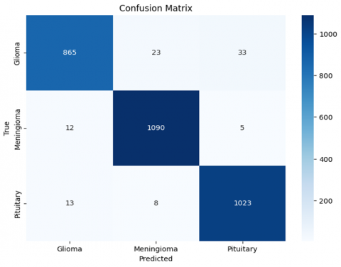
Figure 7. Confusion matrices of the proposed model
The proposed confusion matrix result is shown in Figure 7. When considering the type of Pituitary test images of 1044 and spotting the matrix horizontally, the 1023 images are predicted properly as Pituitary by classifier. It wrongly classified the remaining 21 images of Pituitary: 13 as glioma and 8 as meningioma.
Table 8 provides a summary of performance results in terms of accuracy percentages for various classifier models. DenseUnetGAN attained the accuracy of 95.32. It shows promising performance in generating high-quality output or making accurate predictions. Other models such as CapsNet, CNN, CGan, GAN - random split, VAE GAN, DeLiGAN, and GAN achieved accuracies ranging from 81.6% to 92.6%.
Table 9 presents a Comparative analysis of Results for Brain Tumor Classification along with standard benchmark models. The proposed DenseUnetGAN model achieved the highest accuracy at 95.3%, outperforming all other models. U-Net followed with an accuracy of 92.1%. The DenseNet achieved 92.7%. The 3D U-Net model recorded an accuracy of 93.2%, and ResNet achieved 91.2%. V-Net had an accuracy of 90.8%, and SegNet showed the lowest accuracy at 88.9%. Thus, the proposed model showed the best results in terms of accuracy.
To assess the performance robustness and variability of the DenseUnetGAN model, statistical analysis was conducted on the classification metrics across different tumor types. The parameters used for the statistical analysis include mean, standard deviation (SD), and 95% confidence intervals (CI). The results are given in Table 10.
The DenseUnetGAN model shows high recall, accuracy, and precision across all tumor types. The low standard deviations across metrics highlight the model's stable and reliable performance in tumor classification.
Table 8. Performance analysis of different classifier models
|
Method |
Accuracy |
|
CapsNet |
90.8 |
|
CNN |
88.6 |
|
CGan |
92.6 |
|
GAN |
81.6 |
|
DeLiGAN |
82.5 |
|
GAN -random split |
85.6 |
|
VAE‑GAN |
92.3 |
|
DenseUnetGAN |
95.32 |
Table 9. Comparative results for brain tumor classification
|
Model |
Accuracy (%) |
Dice Similarity Coefficient (DSC) |
IoU |
Precision |
Recall |
F1-Score |
|
DenseUnetGAN (Proposed) |
95.3 |
0.88 |
0.82 |
0.91 |
0.88 |
0.89 |
|
U-Net |
92.1 |
0.85 |
0.80 |
0.89 |
0.86 |
0.87 |
|
ResNet [33] |
91.2 |
0.83 |
0.78 |
0.87 |
0.84 |
0.85 |
|
DenseNet [30] |
92.7 |
0.86 |
0.81 |
0.90 |
0.87 |
0.88 |
|
V-Net [31] |
90.8 |
0.80 |
0.75 |
0.85 |
0.82 |
0.83 |
|
3D U-Net [32] |
93.2 |
0.87 |
0.81 |
0.89 |
0.87 |
0.88 |
|
SegNet [34] |
88.9 |
0.77 |
0.72 |
0.83 |
0.79 |
0.81 |
Table 10. Statistical analysis of classification results for DenseUnetGAN
|
Metric |
Tumor Type |
Mean (%) |
SD (%) |
95% CI Lower Bound (%) |
95% CI Upper Bound (%) |
|
Recall |
Glioma |
98.89 |
1.2 |
97.89 |
99.89 |
|
Meningioma |
94.44 |
1.4 |
93.04 |
95.84 |
|
|
Pituitary |
88.77 |
1.8 |
86.97 |
90.57 |
|
|
Accuracy |
Glioma |
95.76 |
1.0 |
94.86 |
96.66 |
|
Meningioma |
98.49 |
0.9 |
97.74 |
99.24 |
|
|
Pituitary |
98.90 |
0.8 |
98.10 |
99.70 |
|
|
Precision |
Glioma |
95.78 |
1.5 |
94.28 |
97.28 |
|
Meningioma |
91.37 |
1.6 |
89.77 |
92.97 |
|
|
Pituitary |
97.80 |
0.7 |
97.05 |
98.55 |
This paper proposed a hybrid model for brain tumor classification using DenseUnetGAN. By incorporating pre-trained models in the generator and discriminator components, aimed to overcome the limitations of limited data availability in medical imaging datasets. The generator is performed by modified U-Net architecture, while the DenseNet model is utilized as the discriminator and classifier after modifying the fully connected layers. Through extensive experimentation and evaluation, the proposed approach is accurately distinguishing between different tumor classes. The results obtained from experiments highlight the potential of proposed techniques in improving the identification of brain tumors. One significant limitation of the proposed GAN-based approach is its handling of class imbalance. The proposed GAN-based approach may exacerbate class imbalance by generating biased synthetic images that reflect the dominant class distribution. Moreover, GAN training is computationally expensive, requiring significant resources that may not be available in all settings. Future work could focus on addressing class imbalance by incorporating strategies such as adaptive loss functions or using GAN-generated images for oversampling underrepresented classes.
[1] DeAngelis, L.M. (2001). Brain tumors. New England Journal of Medicine, 344(2): 114-123. https://doi.org/10.1056/NEJM200101113440207
[2] Litjens, G., Kooi, T., Bejnordi, B.E., Setio, A.A.A., Ciompi, F., Ghafoorian, M., van der Laak, J.A.W.M., van Ginneken, B., Sanchez, C.I. (2017). A survey on deep learning in medical image analysis. Medical Image Analysis, 42: 60-88. https://doi.org/10.1016/j.media.2017.07.005
[3] Bauer, S., Wiest, R., Nolte, L.P., Reyes, M. (2013). A survey of MRI-based medical image analysis for brain tumor studies. Physics in Medicine & Biology, 58(13): R97. https://doi.org/10.1088/0031-9155/58/13/R97
[4] Dandıl, E., Çakıroğlu, M., Ekşi, Z. (2015). Computer-aided diagnosis of malign and benign brain tumors on MR images. In ICT Innovations 2014: World of Data, Ohrid, North Macedonia, pp. 157-166. https://doi.org/10.1007/978-3-319-09879-1_16
[5] Pereira, S., Pinto, A., Alves, V., Silva, C.A. (2016). Brain tumor segmentation using convolutional neural networks in MRI images. IEEE Transactions on Medical Imaging, 35(5): 1240-1251. https://doi.org/10.1109/TMI.2016.2538465
[6] Goodfellow, I., Pouget-Abadie, J., Mirza, M., Xu, B., Warde-Farley, D., Ozair, S., Courville, A., Bengio, Y. (2020). Generative adversarial networks. Communications of the ACM, 63(11): 139-144. https://doi.org/10.1145/3422622
[7] Vidyarthi, A., Agarwal, R., Gupta, D., Sharma, R., Draheim, D., Tiwari, P. (2022). Machine learning assisted methodology for multiclass classification of malignant brain tumors. IEEE Access, 10: 50624-50640. https://doi.org/10.1109/ACCESS.2022.3172303
[8] Yu, W., Kang, H., Sun, G., Liang, S., Li, J. (2022). Bio-inspired feature selection in brain disease detection via an improved sparrow search algorithm. IEEE Transactions on Instrumentation and Measurement, 72: 2500515. https://doi.org/10.1109/TIM.2022.3228003
[9] Yang, Q., Guo, X., Chen, Z., Woo, P.Y., Yuan, Y. (2022). D ̂2-Net: Dual disentanglement network for brain tumor segmentation with missing modalities. IEEE Transactions on Medical Imaging, 41(10): 2953-2964. https://doi.org/10.1109/TMI.2022.3175478
[10] Sultan, H.H., Salem, N.M., Al-Atabany, W. (2019). Multi-classification of brain tumor images using deep neural network. IEEE Access, 7: 69215-69225. https://doi.org/10.1109/ACCESS.2019.2919122
[11] Huang, Z., Du, X., Chen, L., Li, Y., Liu, M., Chou, Y., Jin, L. (2020). Convolutional neural network based on complex networks for brain tumor image classification with a modified activation function. IEEE Access, 8: 89281-89290. https://doi.org/10.1109/ACCESS.2020.2993618
[12] Asif, S., Yi, W., Ain, Q.U., Hou, J., Yi, T., Si, J. (2022). Improving effectiveness of different deep transfer learning-based models for detecting brain tumors from MR images. IEEE Access, 10: 34716-34730. https://doi.org/10.1109/ACCESS.2022.3153306
[13] Shah, H.A., Saeed, F., Yun, S., Park, J.H., Paul, A., Kang, J.M. (2022). A robust approach for brain tumor detection in magnetic resonance images using finetuned efficientnet. IEEE Access, 10: 65426-65438. https://doi.org/10.1109/ACCESS.2022.3184113
[14] Rizwan, M., Shabbir, A., Javed, A.R., Shabbir, M., Baker, T., Obe, D.A.J. (2022). Brain tumor and glioma grade classification using Gaussian convolutional neural network. IEEE Access, 10: 29731-29740. https://doi.org/10.1109/ACCESS.2022.3153108
[15] Imtiaz, T., Rifat, S., Fattah, S.A., Wahid, K.A. (2019). Automated brain tumor segmentation based on multi-planar superpixel level features extracted from 3D MR images. IEEE Access, 8: 25335-25349. https://doi.org/10.1109/ACCESS.2019.2961630
[16] Zhou, Z., Siddiquee, M.M.R., Tajbakhsh, N., Liang, J. (2019). Unet++: Redesigning skip connections to exploit multiscale features in image segmentation. IEEE Transactions on Medical Imaging, 39(6): 1856-1867. https://doi.org/10.1109/TMI.2019.2959609
[17] Micallef, N., Seychell, D., Bajada, C.J. (2021). Exploring the u-net++ model for automatic brain tumor segmentation. IEEE Access, 9: 125523-125539. https://doi.org/10.1109/ACCESS.2021.3111131
[18] Alhassan, A.M., Zainon, W.M.N.W. (2020). BAT algorithm with fuzzy C-ordered means (BAFCOM) clustering segmentation and enhanced capsule networks (ECN) for brain cancer MRI images classification. IEEE Access, 8: 201741-201751. https://doi.org/10.1109/ACCESS.2020.3035803
[19] Gumaei, A., Hassan, M.M., Hassan, M.R., Alelaiwi, A., Fortino, G. (2019). A hybrid feature extraction method with regularized extreme learning machine for brain tumor classification. IEEE Access, 7: 36266-36273. https://doi.org/10.1109/ACCESS.2019.2904145
[20] Ferdous, G.J., Sathi, K.A., Hossain, M.A., Hoque, M.M., Dewan, M.A.A. (2023). LCDEiT: A linear complexity data-efficient image transformer for MRI brain tumor classification. IEEE Access, 11: 20337-20350. https://doi.org/10.1109/ACCESS.2023.3244228
[21] Noreen, N., Palaniappan, S., Qayyum, A., Ahmad, I., Imran, M., Shoaib, M. (2020). A deep learning model based on concatenation approach for the diagnosis of brain tumor. IEEE Access, 8: 55135-55144. https://doi.org/10.1109/ACCESS.2020.2978629
[22] Mishra, A., Jha, R., Bhattacharjee, V. (2023). SSCLNet: A self-supervised contrastive loss-based pre-trained network for brain MRI classification. IEEE Access, 11: 6673-6681. https://doi.org/10.1109/ACCESS.2023.3237542
[23] Afshar, P., Plataniotis, K.N., Mohammadi, A. (2019). Capsule networks for brain tumor classification based on MRI images and coarse tumor boundaries. In ICASSP 2019-2019 IEEE International Conference on Acoustics, Speech and Signal Processing (ICASSP), Brighton, UK, pp. 1368-1372. https://doi.org/10.1109/ICASSP.2019.8683759
[24] Mirza, M., Osindero, S. (2014). Conditional generative adversarial nets. arXiv preprint arXiv:1411.1784. https://doi.org/10.48550/arXiv.1411.1784
[25] Gurumurthy, S., Kiran Sarvadevabhatla, R., Venkatesh Babu, R. (2017). Deligan: Generative adversarial networks for diverse and limited data. In 2017 IEEE Conference on Computer Vision and Pattern Recognition (CVPR), Honolulu, HI, USA, pp. 4941-4949. https://doi.org/10.1109/CVPR.2017.525
[26] Ghassemi, N., Shoeibi, A., Rouhani, M. (2020). Deep neural network with generative adversarial networks pre-training for brain tumor classification based on MR images. Biomedical Signal Processing and Control, 57: 101678. https://doi.org/10.1016/j.bspc.2019.101678
[27] Ge, C., Gu, I.Y.H., Jakola, A.S., Yang, J. (2020). Enlarged training dataset by pairwise GANs for molecular-based brain tumor classification. IEEE Access, 8: 22560-22570. https://doi.org/10.1109/ACCESS.2020.2969805
[28] Yerukalareddy, D.R., Pavlovskiy, E. (2021). Brain tumor classification based on mr images using GAN as a pre-trained model. In 2021 IEEE Ural-Siberian Conference on Computational Technologies in Cognitive Science, Genomics and Biomedicine (CSGB), Novosibirsk-Yekaterinburg, Russia, pp. 380-384. https://doi.org/10.1109/CSGB53040.2021.9496036
[29] Ahmad, B., Sun, J., You, Q., Palade, V., Mao, Z. (2022). Brain tumor classification using a combination of variational autoencoders and generative adversarial networks. Biomedicines, 10(2): 223. https://doi.org/10.3390/biomedicines10020223
[30] Chauhan, T., Palivela, H., Tiwari, S. (2021). Optimization and fine-tuning of DenseNet model for classification of COVID-19 cases in medical imaging. International Journal of Information Management Data Insights, 1(2): 100020. https://doi.org/10.1016/j.jjimei.2021.100020
[31] Milletari, F., Navab, N., Ahmadi, S.A. (2016). V-net: Fully convolutional neural networks for volumetric medical image segmentation. In 2016 Fourth International Conference on 3D Vision (3DV), Stanford, CA, USA, pp. 565-571. https://doi.org/10.1109/3DV.2016.79
[32] Huang, C., Han, H., Yao, Q., Zhu, S., Zhou, S.K. (2019). 3D U ̂2-Net: A 3D universal U-Net for multi-domain medical image segmentation. In International Conference on Medical Image Computing and Computer-Assisted Intervention, Shenzhen, China, pp. 291-299. https://doi.org/10.1007/978-3-030-32245-8_33
[33] Cheng, J., Tian, S., Yu, L., Gao, C., Kang, X.J., Ma, X., Wu, W.D., Liu, S.J., Lu, H.C. (2022). ResGANet: Residual group attention network for medical image classification and segmentation. Medical Image Analysis, 76: 102313. https://doi.org/10.1016/j.media.2021.102313
[34] Ejiyi, C.J., Qin, Z., Ukwuoma, C., Agbesi, V.K., Oluwasanmi, A., Al-antari, M.A., Bamisile, O. (2024). A unified 2D medical image segmentation network (SegmentNet) through distance-awareness and local feature extraction. Biocybernetics and Biomedical Engineering, 44(3): 431-449. https://doi.org/10.1016/j.bbe.2024.06.001
[35] Radford, A., Metz, L., Chintala, S. (2015). Unsupervised representation learning with deep convolutional generative adversarial networks. arXiv preprint arXiv:1511.06434. https://doi.org/10.48550/arXiv.1511.06434
[36] Ganesamoorthy, B.N., Sakthivel, D.S., Balasubadra, K. (2024). Hen maternal care inspired optimization framework for attack detection in wireless smart grid network. International Journal of Informatics and Communication Technology, 13(1): 123-130. https://doi.org/10.11591/ijict.v13i1.pp123-130
[37] Abasi, A.K., Makhadmeh, S.N., Al-Betar, M.A., Alomari, O.A., et al. (2022). Lemurs optimizer: A new metaheuristic algorithm for global optimization. Applied Sciences, 12(19): 10057. https://doi.org/10.3390/app121910057
[38] Cheng, J., Huang, W., Cao, S., Yang, R., Yang, W., Yun, Z.Q., Wang, Z.J., Feng, Q.J. (2015). Enhanced performance of brain tumor classification via tumor region augmentation and partition. PloS One, 10(10): e0140381. https://doi.org/10.1371/journal.pone.0140381
[39] Marcus, D.S., Fotenos, A.F., Csernansky, J.G., Morris, J.C., Buckner, R.L. (2010). Open access series of imaging studies: Longitudinal MRI data in nondemented and demented older adults. Journal of Cognitive Neuroscience, 22(12): 2677-2684. https://doi.org/10.1162/jocn.2009.21407