Rashmi Saini*![]() | Shivam Rawat
| Shivam Rawat![]() | Prabhakar Semwal
| Prabhakar Semwal![]() | Suraj Singh
| Suraj Singh![]() | Surendra Singh Chaudhary
| Surendra Singh Chaudhary![]() | Tushar Hrishikesh Jaware
| Tushar Hrishikesh Jaware![]() | Kanubhai K. Patel
| Kanubhai K. Patel![]()
© 2024 The authors. This article is published by IIETA and is licensed under the CC BY 4.0 license (http://creativecommons.org/licenses/by/4.0/).
OPEN ACCESS
Built-up mapping possesses a great challenge owing to the varying spectral signatures and spatial attributes of different features such as buildings, individual houses, roads, etc. Here, the key challenge is to separate built-up class and bare/fallow land class due to the spectral signature similarity. The objectives of this study are as follows: (i) to extract built-up features using spectral bands and twelve popular spectral indices using advanced machine learning techniques and analyzing the change in accuracy after integrating selected spectral indices in the classification, (ii) separability analysis of built-up class and bare/fallow land using the Spectral Discrimination Index (SDI) and histogram plots for selected indices. (iii) the performance of the advanced ensemble classifier, extreme gradient boosting, is compared to other well-known machine learning techniques, such as Random Forest, Support Vector Machine, and K-nearest neighbors (KNN). Two datasets were used: Dataset-1 was formed by performing stacking operation on four bands at 10 m spatial resolution. Dataset-2 was prepared by computing twelve spectral indices and integrating them with Dataset-1. The results indicated that extreme gradient boosting method obtained highest overall accuracy and kappa value of 88.90%, 0.848 for Dataset-1, and 94.30%, 0.922 for Dataset-2, respectively. The overall accuracy for Random Forest, Support Vector Machine, and KNN is 88.23%, 87.05%, and 86.60% for Dataset-1, and 93.04%, 91.04%, and 89.93% for Dataset-2, respectively. There is a significant rise of 4.81% (Random Forest), 3.99% (Support Vector Machine), 3.33% (KNN), and 5.40% (extreme gradient boosting) in overall accuracy for the fused dataset has been observed. The outcome of this study suggest that the Enhanced Normalized Difference Impervious Surfaces Index (ENDISI) and Modified Normalized Difference Water Index (MNDWI) are very useful spectral indices for mapping of built-up with a higher degree of separability for built-up and bare/fallow land separation.
built-up, satellite image, extreme gradient boosting, K-nearest neighbors, machine learning, Random Forest, spectral indices, Support Vector Machine
There has been a great expansion of impervious surfaces over the last few decades due to rapid urbanization, and industrialization. Impervious surfaces or built-up are man-made structures such as built-up surfaces, concrete structures, roadways, freeways, highways, and parking lots that are water resistant [1]. The information about impervious surface distribution is helpful in many applications, such as population analysis, building extraction, and land use analysis [2-5]. Furthermore, this information aids in comprehending the environmental impact of impervious surfaces [6]. Urban heat islands are formed when open green permeable spaces are replaced with impermeable infrastructures such as buildings, houses, roads, etc. It is an area where the temperature is considerably higher than the surrounding rural areas as a result of the release of heat trapped by impervious surfaces [7, 8]. Impervious surfaces disrupt the cycle of atmospheric carbon because they displace biological vegetation, which lowers ecological output. The uncontrolled expansion of impervious surfaces can lead to various problems, such as the problem of water-logging due to surface water run-off [9], a decrease in the level of groundwater due to the non-porous nature of impervious surfaces [10], and deterioration of the water resources [11], which can disturb the natural water-cycle [12].
Remote sensing and space technology advancements in recent years have opened avenues for effective land use/cover mapping owing to powerful machine learning (ML) algorithms and the availability of high-quality, freely available satellite data. A few of these popular satellites, such as Landsat, Sentinel-2, Worldview, and IKONOS, provide high-quality data with very good temporal and spatial resolution, which are important characteristics for an effective land cover mapping scheme. However, mapping built-up and impervious surfaces possess a great challenge because of different reasons. For example, built-up surfaces are made of various materials, such as concrete, cement, gravel, brick, coal tar, and metal, and their spectral signatures can be identical to those of other materials, such as bare/fallow land, silt, etc. [8, 13].
The conventional method for built-up extraction is an exhausting process that requires human expertise, field surveys, and the use of historical data [14]. There are different classification techniques used for urban mappings, such as hard classification methods (unsupervised, semi-supervised, and supervised), and soft classification methods (fuzzy-based) [15, 16]. The unsupervised classification method for built-up extraction is not a very popular method owing to poor classification accuracy [17]. Literature indicated that use of spectral indices is one popular method for built-up extraction. However, the problem with spectral indices is that they are subject to vary with the seasons, and sometimes, there may be a misclassification of built-up areas with bare/fallow land areas because of the spectral homogeneity between the two [18]. The various other methods to extract impervious surfaces are spectral mixture-based analysis [19], image segmentation [20], ensemble-based learning [21], multiple regression [22], and Gray Level Co-occurrence Matrice (GLCM) features [23]. The fusion technique using different satellite datasets such as optical/radar data is another promising technique of image classification that combines spectral bands with various other features such as spectral and textural features [24-27]. Joshi et al. [28] performed a brief literature review of 32 papers on satellite image fusion and found that 28 out of 32 studies reported an increase in the classification accuracy for different land cover studies using the fused dataset. In order to understand the impact of fusion, 12 popular spectral indices have been computed and fused with the four-band Sentinel-2 dataset in this study.
In the past few decades, machine learning algorithms have gained immense popularity owing to their robust performance and faster execution time. These algorithms have been used extensively with different optical satellite datasets such as low spatial resolution datasets (MODIS, AVHRR) [29], medium spatial resolution datasets (Landsat) [30], and very high-resolution imagery (QuickBird, Ikonos) [31, 32]. The optical satellite however cannot penetrate clouds. As such, Synthetic Aperture Radar (SAR) data has become popular due to its unique ability to penetrate clouds [33, 34]. Very few studies have exploited the potential of high-resolution satellite datasets for built-up mapping [35]. High-resolution imagery can address the problems of mixed pixels arising due to low-resolution imagery and thereby increase classification accuracy [36]. Besides this, the classification performance is influenced by many factors, such as the complexity of the research area, the spatial/spectral/temporal resolution of the satellite, and seasonal variability [37-39].
The recently launched (Sentinel 2A and 2B) passive optical satellites provide multispectral data useful for land cover mapping and other applications because of high spatial/temporal resolution, short revisit times, and free data availability [39]. The multispectral bands of the Sentinel-2 data are available at 10 m spatial resolution that can be effectively used for mapping of built-up areas in comparison to the Landsat series data [40, 41]. Non-parametric algorithms (Decision Tree, RF, SVM, and knowledge-based learning methods) have proven to be extremely useful in recent decades when compared to traditional classifiers such as maximum likelihood due to their robust performance and good fault tolerance [42, 43]. Das et al. [44] used four ML algorithms, i.e., RF, SVM, Artificial Neural Network (ANN), and Gradient Boosting, to extract building features using very high-resolution imagery. This study found that ANN performed considerably in linear homogeneous building distribution. RF, on the other hand, demonstrated great accuracy in the non-linear and diverse dispersion of urban buildings. Barman and Mustak [45] used SVM with linear and Radial basis function (RBF) kernel to extract the building footprints of Kolkata city in India. Abdi [46] used four ML algorithms (RF, SVM, XGBoost, and Deep learning (DL)) to obtain effective classification results. The results indicated that SVM gave the best performance followed by XGBoost, RF, and DL. Hence, most of the studies suggested the use of non-parametric ML classifiers for built-up extraction owing to robust performance and faster execution.
Spectral indices derived from the spectral bands can be calculated using various mathematical equations that minimize the impact of shadow due to clouds or mountains and enhance the spectral characteristics of the image. The efficiency and performance of these spectral indices vary with respect to study areas owing to different topography and geographical conditions. Chen et al. [47] used six different indices to extract built-up area on different study areas using different ML algorithms. The results indicated that the biophysical composition index (BCI) and combinational build-up index (CBI) were disturbed by the presence of water bodies while three indices (combinational biophysical composition index (CBCI), index-based built-up index (IBI), and normalized difference built-up index (NDBI) were influenced by study area. ENDISI gave the best performance among all six indices with a higher degree of separability and overall accuracy of 91%. Shi et al. [48] found that Impervious surface extraction using Sentinel-2 had reported less error than those created using Landsat data WorldView-3 as well. Valdiviezo-N et al. [49] discussed various built-up indices techniques along with their applications for urban extraction. The results have shown that built-up indices gave a better performance in moist/humid seasons. Osgouei et al. [50] used a combination of indices for built-up mapping which gave better results in comparison to the ten-band Sentinel-2 dataset. Kebedea et al. [51] extracted impervious surfaces based on SDI on Sentinel-2 images by using 7 different built-up indices using an SVM classifier. The results indicated that spectral indices can be used to extract impervious surfaces efficiently. Previously, similar studies based on SDI and histogram overlap were conducted [52, 53].
Literature indicated that accurate built-up extraction is a challenging task in the domain of remote sensing and it becomes more critical as different LULC classes have signature overlapping issue. It has been observed from the literature that the potential of SDI is not properly investigation in the area of built-up extraction. In addition, it is also found that the efficiency of advance ensemble technique such as extreme gradient boosting has not been utilized with the fused dataset to obtain effective built-up maps.
This paper aims to understand the impact of different spectral indices on a few popular machine learning classifiers for built-up extraction. Furthermore, to analyze the separability between the bare/fallow land and built-up areas, a few statistical measures such as the SDI and histogram have been utilized. The main objective is to map built-up surfaces using pixel-based, supervised ML classification techniques. The following are the research objectives that are covered in this study:
This paper is organized in the follower manner: Section 2 describe the material and methods adopted for this research work, this section consists of two sub-sections, first one describes the selected study area and second sub-section presents the pre-processing required for data. Section 3 demonstrates the methodology used in this study. The methodology section discusses step-by-step workflow of the study and also provide a brief description of all the ML classifiers (KNN, SVM, RF and XGBoost) used in the study. This section also presents the SDI, as well as discusses Spectral Curve Analysis for various LULC class. Section 4 presents the results and provide in-depth analysis of the outcomes obtained in the study. Section 5 emphasizes on the major conclusions of the study.
Figure 1. (a) Study area located in Maharashtra, India; (b) Maharashtra state district-wise division; (c) Study area boundary; (d) Study area in false color Composite; (e) Study area shown as the true color composite of surface reflectance images of 12th January 2021
2.1 Study area
In this research work, the chosen study area is the Mumbai sub-urban district. This city is located in the Konkan Division of Maharashtra state, India. In the state of Maharashtra, it is the second smallest district. Here the population of the study area is 9.36 million. This study site i.e. Mumbai suburban district is covered by the 19° 16' 7.6872"N to 18° 58' 43.7268"N latitude and 72°46' 33.0492"E to 72° 58' 49.656"E longitude of spatial dimension. In the fast growing developing country, infrastructure is growing at a rapid rate, due to which small town are continuously converting into the big cities. At the same time the agricultural land is converting into high rise building and industrial area. In the field of remote sensing a huge variety of satellite datasets are available to address various classification problems. The commonly used satellite datasets are Landsat series, SPOT Sentinel-1, 2, Rapid Eye, Worldview datasets are available to address different sets of applications. To address this specific application for built-up mapping we require a medium spatial resolution dataset. Therefore, Sentinel-2 dataset has been chosen as it provides the freely available data at 10m spatial resolution. In order to obtain the effective classification maps, it is necessary that the input imagery must be cloud free or with minimum cloud cover. For this research work, Sentinel-2 dataset of 12th January 2021 were utilized. Figure 1 demonstrated the selected study area located in the Maharashtra state of India. Here for better representation, False Color Composite (FCC) format and True Color Composite (TCC) format both are shown along with the location of study area in state and country.
2.2 Pre-processing of data
The Sentinel-2A and Sentinel-2B are twin optical satellites which were launched by European Space Agency (ESA) in the year 2015 and 2017 respectively [54]. There are thirteen spectral bands provided by the Sentinel-2 dataset (4 bands at 10 m spatial resolution (Red (R), Blue (B), Green (G), and Near Infrared Band (NIR)), six bands at 20m spatial resolution (Veg. (RE)1 Band 5), (Veg. (RE)2 Band 6), (Veg. (RE)3 Band 7), Vegetation Red Edge (8A), Short Wave Infrared Band 1 (SWIR-1), Short Wave Infrared Band 2 (SWIR-2)), and three bands at 60m spatial resolution (Coastal Aerosols, Water Vapor, and Short Wave Infrared Cirrus)). Scientist and researchers around the world utilized Sentinel-2 dataset for different land use/cover studies, such as crop/vegetation mapping [55, 56], flood mapping [57, 58], forest classification [59, 60], surface water mapping [61, 62], etc. The images were acquired in Level-1C Top of Atmospheric (TOA) conditions in UTM Zone 43 N projection under a clear sky with a minimum cloud cover. The Level-1C images suffer from the effects of absorption and scattering, for which there is a need to pre-process them. Pre-processing is a crucial step to retain the true values of surface reflectance, the images need to be atmospherically corrected. The pre-processing operations were carried out using Sen2cor processor [63]. After pre-processing, the images are converted to Level-2A (Bottom of the Atmosphere format), which can be used for further analysis.
This study implemented four machine learning techniques for mapping of built-up area from other LULC classes. A brief description of all machine learning classifiers has been provided in the subsequent section.
3.1 Random Forest
Breiman [64] introduced a widely used ML technique that integrates the technique of bootstrapping with feature selection procedures to generate decision trees, with different trees generating a subset of features and training data after replacement. Because of this, there is a decrease in the variance which increases the overall performance of the classifier. It can be used with categorical as well as continuous variables. It can be used for classification and regression tasks.
The unlabeled data is categorized based on a voting scheme. The most common voting mechanism is majority voting. The RF classifier is one of the top-performing classifiers since it is simple to parameterize and avoids overfitting [65]. The RF model's performance is defined by two primary factors:
• Ntree: number of trees used in aggregation.
• Mtry: number of randomly selected features or predictors used to separate the nodes.
3.2 Support Vector Machine
Vapnik and Chervonenkis [66] proposed this algorithm and implemented it as a binary linear classifier. Thereafter, Vapnik [67] made some changes to modify this in order to obtain better performance. It finds an optimal hyperplane that distinguishes data points with the greatest margin or distance between the two classes (known as a maximum-margin hyperplane). It is space efficient and works efficiently even when training data samples are small. The type of kernel used for SVM implementation has a significant impact on its performance. Depending upon the types of applications, different kernels are available such as linear, sigmoid, string function, graph, etc. [68].
3.3 KNN
KNN is a robust and popular ML algorithm that categorizes the test data samples from the available class labels by measuring the distance between the test samples and k nearest trained samples [69]. The distance can be calculated using different metrics (Minkowski, Euclidean, and Manhattan), of which the Euclidean distance is the most popular distance metric. Here, K, a tuning parameter, regulates how well the classifier performs. A high value of K over fits the model while a low value will give an unstable decision boundary [70].
3.4 Extreme gradient boosting
The first description of this algorithm was given by Tianqi and Carlos in 2016 [71]. Boost is an improvised scalable version [72] of GBM (Gradient Boosting Machine) that works by building various models that are initially weak learners and make weaker predictions. These weak learning models are used to make stronger models that make better predictions. It works by defining an objective function that uses a loss function in combination with a regularization parameter that enables parallelism, thereby increasing the computation speed of the model. Different objective functions are available, such as softmax, hardmax, etc. The advantage of XGBoost is that it supports parallel computations and is ten times faster than conventional GBM. Various studies have shown the comparable and better performance of XGB Boost over the traditional classifiers such as RF and SVM [73, 74].
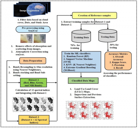
Figure 2 illustrates the proposed methodology. The proposed methodology consists of following major steps: (i) Data Acquisition and pre-processing, (ii) Creation of reference data samples, (iii) Implementation and training of machine learning classifiers, (iv) Assessment of accuracy for each ML model. In this work, a supervised machine learning classification technique is used for Land Use/Cover Classification (LULC) on Sentinel-2 datasets. Each ML model has been trained with the reference dataset. This reference dataset has been created using Google Earth imagery. For this study, two datasets have been created. The first dataset, referred to as Dataset-1, has been formed by stacking four spectral bands i.e. R (10m), G (10m), B (10m), and NIR (10m)). For the second dataset, referred to as Dataset- 2, twelve spectral indices (Table 1) have been computed, thereafter these computed indices are integrated with Dataset-1 to form Dataset-2. Studies have shown that down-sampling results in better classification accuracy compared to up-sampling, which also helps in preserving spectral information [75, 76]. To calculate a few indices that involve the usage of Shortwave Infrared Bands (Shortwave IR1 (20m) and Shortwave IR2 (20m)) were down-sampled to 10m spatial resolution. In this study, four machine learning algorithm namely RF, SVM KNN and XGBoost have been used. Literature indicated that RF and SVM are most popular ML algorithm used for a wide range of classification problem using satellite data [23, 25, 55, 56, 58, 68]. KNN has been used as a baseline classifier. In addition, this study considered advance ensemble classifier i.e. XGBoost. It has been observed that very few studies utilized the XGBoost classifier using satellite imagery. Therefore, in this study, we have chosen XGBoost classifier to explore its potential for effective built-up extraction and compare its performance with well-known ML classifier.
To evaluate the performance of ML classifiers various accuracy measures have been used such as overall accuracy and kappa coefficient are computed as an overall measure for a classifier. Whereas, precision and recall are computed for a specific LULC class for each classifier. These values are calculated using True Positive (TP), True Negative (TN), False Positive (FP) and False Negative (FN). Kappa Coefficient is popular measure utilized for various remote sensing. Kappa value varies from 0 to 1. This measure demonstrates the difference between the actual agreement and the agreement expected by chance. A higher value of kappa 1 indicated that the resultant classified image and the reference image are identical. Therefore, the higher value of kappa is desirable. The above discussed accuracy measures are calculated using Eqs. (1)-(4) respectively.
Accuracy =TP+TNTP+TN+FN+FP (1)
Precision =TPTP+FP (2)
Recall =TPTP+FN (3)
kappa = observed accuracy − chance agreement 1− chance agreement (4)
Table 1. Various indices and their description
|
Index ID |
Index Name |
Bands Used |
Advantages/ Disadvantages |
References |
|
ENDISI |
Enhanced Normalized Difference Impervious Surfaces Index |
Blue, Green, SWIR1, |
It can reduce the impact of arid land, bare rock, and soil on impervious surfaces efficiently. |
Chen et al. [77] |
|
NDBI |
Normalized Difference Built-up Index |
NIR, SWIR1 |
It is similar to NDVI but achieves lower accuracy for built-up extraction. |
Zha et al. [78] |
|
BRBA |
Band Ratio for Built-up Area |
Green, NIR |
It was used to separate bare land and built-up areas on Landsat data. |
Waqar et al. [79] |
|
SAVI |
Soil Adjusted Vegetation Index |
Red, NIR |
It is used to adjust the plant density in a given region with the help of a correction factor. |
Huete [80] |
|
NDVI |
Normalized Difference Vegetation Index |
Red, NIR |
It is used to determine crops’ health status. |
Rouse et al. [81] |
|
MNDWI |
Modified Normalized Difference Water Index |
Green, SWIR1 |
It is used to highlight water bodies in urban areas. |
Xu et al. [82] |
|
BSI |
Bare land Index |
Blue, Red, NIR, SWIR1 |
It can capture soil variation and enhance bare land and fallow land. |
Roy et al. [83] |
|
NDCCI |
Normalized Difference Concrete Condition Index |
NIR, Green |
It is used to determine the built-up material condition. |
Samsudin et al. [84] |
|
NBAI |
Normalized Built-up Area Index |
Green, SWIR1, SWIR2 |
It is used to delineate bare land and built-up area. |
Waqar et al. [79] |
|
NBI |
New Built-up Index |
Red, NIR, SWIR2 |
It was used to extract residential areas in Changzhou, China. |
Chen et al. [85] |
|
UI |
Urban Index |
NIR, SWIR1 |
It is used for evaluating urbanization. |
Kawamura et al. [86] |
|
OSAVI |
Optimized Soil Adjusted Vegetation Index |
Red, NIR |
It was created to compensate for soil variability. |
Rondeaux et al. [87] |
4.1 Spectral discrimination index
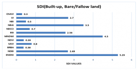
Mapping of built-up and impervious surfaces possess a great challenge because of different reasons. For example, built-up surfaces are made of various materials, such as concrete, cement, gravel, brick, coal tar, and metal, and their spectral signatures can be identical to those of other materials, such as bare/fallow land, silt, etc. As such, this study exploits the separability between the two classes using the SDI. The SDI is used to measure the degree of difference between different land cover classes [88]. SDI can be calculated using Eq. (5). Here μ1,μ2 represents the mean index values for classes 1 and 2 respectively, whereas σ1,σ2 represents the standard deviation of classes 1 and 2 respectively. If SDI values are less than 1, there is spectral homogeneity between the classes and the ability to differentiate is poor, whereas if SDI values lie between 1 and 3 histogram means can be well distinguished and classes can be moderately separated. However, if SDI values are greater than 3, there is no overlap between the spectral signatures, and classes can be separated perfectly. Table 2 and Figure 3 show the SDI values obtained for the built-up surfaces and bare/fallow land.
SDI=|μ1−μ2|σ1+σ2 (5)
4.2 Spectral Curve Analysis for different land cover classes
Figure 4 shows that different land cover classes can be easily separated from each other based on their spectral signature. However, it was challenging to separate the bare/fallow land from the built-up areas as they shared a similar spectral signature, and hence it became necessary to investigate their separability using a combination of different spectral indices. The spectral signature curve also shows that the spectral profile of fallow land and built-up areas are almost identical for bands (RE1, RE2, RE3, NIR, Vegetation Red Edge (8A)), indicating a partial separability between the two. Whereas, there was better separability for bands Blue, Green, SWIR1, and SWIR2 for the built-up and fallow land. This also highlights the fact that most of the proposed indices for built-up exploit the characteristics of bands Blue (10m), Green (10m), Red (10m), NIR (10m), SWIR1 (20m), and SWIR2 (20m).
Table 2. Values of SDI between built-up and bare/fallow class
|
|
Spectral Indices |
|||||||||||
|
Spectral Nation Index |
ENDISI |
NDBI |
BRBA |
SAVI |
NDVI |
MNDWI |
BSI |
NDCCI |
NBAI |
NBI |
UI |
OSAVI |
|
SDI (Built-up, Bare/Fallow Land) |
5.29 |
2.69 |
0.38 |
0.8 |
0.39 |
4.5 |
2.56 |
0.7 |
3.5 |
0.5 |
2.7 |
0.3 |
Figure 3. SDI Values between built-up and bare/fallow land for different indices
Figure 4. Spectral signature curve for the selected LULC classes for Sentinel-2 bands
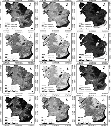
This study aimed to map built-up land cover class using Sentinel-2 imagery and ML models. Evaluation metrics included histogram and Standard Deviation Index. The dataset comprised spectral bands and an integration of spectral indices. Shortwave infrared bands were resampled to 10m spatial resolution using Nearest Neighbors. Stratified random sampling procedure with 70% training and 30% testing was employed. Here, total number of samples is equal to 4503 pixels. For the implementation R programming language has been used. All the ML models have been trained on default values of tuning parameters. Results utilized down-sampling for better classification accuracy and spectral information preservation information [76, 77]. The study enhances understanding of ML classifier performance in built-up feature extraction from Sentinel-2 imagery, with implications for urban mapping and land cover studies. To obtain the classification maps, the first three classes were clubbed together and referred to as “pervious surfaces” while the other class is referred to as “built-up surfaces”. Table 3 shows the accuracy metrics attained for the RF, SVM, KNN and XGBboost. Table 4 shows the feature importance of the spectral bands and spectral indices for the RF, SVM, KNN, and XGBoost classifiers, respectively. All twelve spectral indices are calculated and results are shown in Figure 5.
5.1 Impact of spectral indices on classification
The inclusion of spectral indices resulted in improved classification accuracy, with notable enhancements in overall accuracy (Table 3): 4.81% (RF), 3.99% (SVM), 3.33% (KNN), and 5.40% (XGBoost).
Challenges in built-up surface extraction, particularly misclassification with bare/fallow land, were addressed by spectral indices, with BSI, ENDISI, NDBI, MNDWI, and UI showing the highest SDI values for separation.
Table 3. Accuracy metrics for the Dataset-1 and the Dataset-2
|
Dataset Used |
Classifier Used |
|||||||
|
|
RF |
SVM |
KNN |
XGBoost |
||||
|
(Bands Used) |
OA |
ka |
OA |
ka |
OA |
ka |
OA |
ka |
|
Dataset-1 (Red + Blue + Green + NIR) |
88.23 |
0.84 |
87.05 |
0.824 |
86.60 |
0.818 |
88.90 |
0.849 |
|
Dataset-2 (Red + Blue + Green + 12 Indices) |
93.04 |
0.904 |
91.04 |
0.877 |
89.93 |
0.862 |
94.30 |
0.922 |
Table 4. Variable importance for Dataset-2
|
FEATURES |
RF |
SVM |
KNN |
XGBoost |
|
BLUE |
100 |
91.93 |
91.93 |
100 |
|
GREEN |
28.862 |
76.44 |
76.44 |
32.30 |
|
RED |
49.489 |
89.85 |
89.85 |
54.26 |
|
NIR |
24.581 |
54.73 |
54.73 |
45.49 |
|
ENDISI |
89.94 |
100 |
100 |
83.50 |
|
NDBI |
13.001 |
90.05 |
90.05 |
66.55 |
|
BRBA |
44.844 |
85.48 |
85.48 |
43.85 |
|
SAVI |
0 |
59.7 |
59.7 |
71.05 |
|
NDVI |
38.97 |
86.4 |
86.4 |
61.3 |
|
MNDWI |
16.545 |
70.83 |
70.83 |
98.67 |
|
BSI |
9.697 |
83.63 |
83.63 |
62.52 |
|
NDCCI |
6.45 |
0 |
0 |
33.55 |
|
NBAI |
40.849 |
80.46 |
80.46 |
81.59 |
|
NBI |
28.711 |
99.62 |
99.62 |
42.45 |
|
UI |
14.324 |
90.05 |
90.05 |
70.57 |
|
OSAVI |
11.948 |
69.57 |
69.57 |
0 |
Figure 5. Calculated Indices (a) Endisi, (b) Ndbi, (c) Brba, (d) Savi, (e) Ndvi, (f) Mndwi, (g) Bsi, (h) Ndcci, (i) Nbai, (j) Nbi, (k) Ui, (l) Osavi
5.2 Histogram analysis
One of the biggest challenges while extracting built-up surfaces is the misclassification of the built-up surfaces with the bare/fallow land. The histogram plot has been computed for the calculated indices to realize the separation between the bare/fallow land and built-up areas as they share similar spectral characteristics (Figure 6). The histogram curve for the 12 indices used in this study is displayed in Figure 6.
The results indicate that BSI, ENDISI, NDBI, MNDWI, and UI achieved the highest SDI values of 2.56, 5.29, 2.69, 4.5, and 2.7, respectively, for built-up and bare/fallow land separation. Whereas, BRBA, NDCCI, NBI, OSAVI, and SAVI achieved SDI values of 0.38, 0.7, 0.5, 0.3, and 0.8, respectively.
Histogram plots for various indices revealed that ENDISI and MNDWI effectively separated built-up areas from bare/fallow land, while BSI, NDBI, and UI showed moderate separation.
Indices like BRBA, NDCCI, NBI, OSAVI, and SAVI exhibited overlap, indicating challenges in differentiation.
5.3 Classification results
Four classes were identified: water body, vegetation, fallow land, and built-up areas. Pervious surfaces included water, vegetation, and fallow land, while built-up surfaces comprised roads, parks, and other impervious structures.
Tables 5 and 6 show the accuracy measures for the RF, SVM, KNN, and XGBoost classified dataset for 4-band data and 16-band data respectively.
To assess the performance of classification, various accuracy metrics were calculated (overall accuracy (OA), Kappa score (k), Precision, Recall through the confusion matrices for the respective classifiers.
XGBoost outperformed other classifiers, achieving the highest OA of 88.90% for Dataset-1 and 94.30% for Dataset-2.
The OA obtained for Dataset-1 using RF, SVM, and KNN is 88.23%, 87.05%, and 86.60%, with ka of 0.840, 0.824, and 0.818, respectively. Whereas, for Dataset-2, the OA and ka obtained are 93.04%, 0.904 for RF, 91.04%, 0.877 for SVM, 89.93%, 0.862 for KNN, and 94.30%, 0.922 for XGBoost.
Figure 6. Histograms of different indices showing degrees of overlap between built-up class and bare/fallow land class
Table 5. Accuracy measures obtained by RF, SVM, KNN and XGBoost for Dataset-1
|
|
RF |
SVM |
KNN |
XGBoost |
||||
|
classes |
Precision |
Recall |
Precision |
Recall |
Precision |
Recall |
Precision |
Recall |
|
WB |
100 |
100 |
100 |
99.50 |
100 |
99.5 |
100 |
100 |
|
VG |
96.13 |
99.50 |
97.31 |
99.50 |
96.13 |
99.25 |
96.84 |
99.5 |
|
FL |
64.69 |
91.60 |
61.5 |
88.8 |
60.65 |
90 |
65.53 |
92 |
|
BU |
95.30 |
72.85 |
91.46 |
71.26 |
94.84 |
69.17 |
95.89 |
74.45 |
Table 6. Accuracy measures obtained by RF, SVM, KNN and XGBoost for Dataset-2
|
|
RF |
SVM |
KNN |
XGBoost |
||||
|
classes |
Precision |
Recall |
Precision |
Recall |
Precision |
Recall |
Precision |
Recall |
|
WB |
100 |
100 |
100 |
100 |
100 |
100 |
100 |
100 |
|
VG |
98.52 |
100 |
98.76 |
100 |
98.28 |
100 |
98.76 |
100 |
|
FL |
75.08 |
95.2 |
70 |
92.4 |
67.46 |
90.4 |
78.31 |
96.8 |
|
BU |
97.90 |
83.63 |
95.91 |
79.64 |
95.11 |
77.64 |
98.86 |
86.23 |
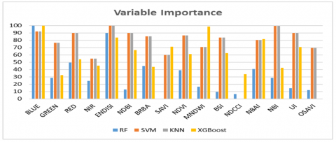
Figure 7. Comparison of the variable importance of classifiers concerning spectral bands and spectral indices
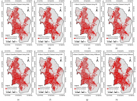
Figure 8. Classification map obtained by all ML classifier, (a), (c), (e), (g) represents 4 band classification results obtained by KNN, RF, SVM and XGBoost respectively. Here, (b), (d), (f), (h) represents 16 band classification map obtained by KNN, RF, SVM and XGBoost respectively
5.4 Variable importance analysis
Feature importance analysis revealed the significant contribution of spectral indices along with spectral bands to classification. There is no model-specific method for calculating the variable importance of KNN and SVM; they are all calculated based on loss squared variable importance, which is identical for both models. Figure 7 displays the comparative analysis of the variable importance of different ML models with respect to the spectral bands and the twelve spectral indices.
Top features varied across classifiers, emphasizing the importance of specific indices, such as ENDISI, MNDWI, BSI, NDBI, and UI.
For RF, the top 5 features were (BLUE = 100%, ENDISI = 89.94%, RED = 49.49%, BRBA = 44.84%, and NBAI = 40.85%).
For KNN and SVM, key features were (ENDISI = 100%, NBI = 99.62%, BLUE = 91.93%, NDBI = 90.05%, and UI = 90.05%).
XGBoost's top features included (BLUE = 100%, MNDWI = 98.67%, ENDISI = 83.5%, NBAI = 81.59%, and SAVI = 71.05%).
5.5 Model limitations
Acknowledging challenges in misclassification with bare/fallow land due to spectral similarity, the study highlights the effectiveness of spectral indices in mitigating this issue.
Further insights into the limitations of the approach, such as potential challenges under specific environmental conditions, could provide a more comprehensive understanding.
5.6 Conclusion and efficacy of approach
The study successfully demonstrated the efficacy of integrating spectral indices with spectral bands in improving built-up surface extraction accuracy.
XGBoost emerged as the top-performing classifier, showcasing the potential of the proposed approach for mapping built-up and impervious surfaces.
The misclassification of built-up areas with bare land was reduced when the dataset was integrated with spectral indices, underscoring the practical utility of this enhancement. Figure 8 displays the KNN, RF, SVM and XGBoost classified data maps obtained for datasets 1 and 2.
The major findings of this study are as follows:
[1] Bauer, M.E., Loeffelholz, B., Wilson, B. (2005). Estimation, mapping and change analysis of impervious surface area by Landsat remote sensing. In: Proceedings, Pecora 16 Conference, South Dakota, US, pp. 23-27.
[2] Wu, K.Y., Zhang, H. (2012). Land use dynamics, built-up land expansion patterns, and driving forces analysis of the fast-growing Hangzhou metropolitan area, eastern China (1978–2008). Applied Geography, 34: 137-145. https://doi.org/10.1016/j.apgeog.2011.11.006
[3] Yang, X.Y., Jiang, G.M., Luo, X.Z., Zheng, Z. (2012). Preliminary mapping of high-resolution rural population distribution based on imagery from Google Earth: A case study in the Lake Tai basin, eastern China. Applied Geography, 32(2): 221-227. https://doi.org/10.1016/j.apgeog.2011.05.008
[4] Wania, A., Kemper, T., Tiede, D., Zeil, P. (2014). Mapping recent built-up area changes in the city of Harare with high resolution satellite imagery. Applied Geography, 46: 35-44. https://doi.org/10.1016/j.apgeog.2013.10.005
[5] You, Y., Wang, S.Y., Ma, Y.X., Chen, G.S., Wang, B., Shen, M., Liu, W.H. (2018). Building detection from VHR remote sensing imagery based on the morphological building index. Remote Sensing, 10(8): 1287. https://doi.org/10.3390/rs10081287
[6] Zhang, H.S., Lin, H., Zhang, Y.Z., Weng, Q.H. (2015). Remote Sensing of Impervious Surfaces in Tropical and Subtropical Areas. CRC Press. https://doi.org/10.1201/b18836
[7] Liqin, C., Li, P.X., Zhang, L.P. (2008). Impact of impervious surface on urban heat island in Wuhan, China. In International Conference on Earth Observation Data Processing and Analysis (ICEODPA), Wuhan, China. https://doi.org/10.1117/12.815911
[8] Thapa, R.B., Murayama, Y. (2009). Urban mapping, accuracy, and image classification: A comparison of multiple approaches in Tsukuba city, Japan. Applied Geography, 29(1): 135-144. https://doi.org/10.1016/j.apgeog.2008.08.001
[9] Thakali, R., Kalra, A., Ahmad, S. (2016). Understanding the effects of climate change on urban stormwater infrastructures in the Las Vegas valley. Hydrology, 3(4): 34. https://doi.org/10.3390/hydrology3040034
[10] Pappas, E.A., Smith, D.R., Huang, C., Shuster, W.D., Bonta, J.V. (2008). Impervious surface impacts to runoff and sediment discharge under laboratory rainfall simulation. CATENA, 72(1): 146-152. https://doi.org/10.1016/j.catena.2007.05.001
[11] Liu, Z.H., Wang, Y.L., Li, Z.G., Peng, J. (2013). Impervious surface impact on water quality in the process of rapid urbanization in Shenzhen, China. Environmental Earth Sciences, 68: 2365-2373. https://doi.org/10.1007/s12665-012-1918-2
[12] Shuster, W.D., Bonta, J., Thurstron, H., Warnemuende, E., Smith, D.R. (2005). Impacts of impervious surface on watershed hydrology: A review. Urban Water Journal, 2(4): 263-275. https://doi.org/10.1080/15730620500386529
[13] Lu, D.S., Moran, E., Hetrick, S. (2011). Detection of impervious surface change with multitemporal Landsat images in an urban-rural frontier. ISPRS Journal of Photogrammetry and Remote Sensing, 66(3): 298-306. https://doi.org/10.1016/j.isprsjprs.2010.10.010
[14] Sun, G.Y., Chen, X.L., Jia, X.P., Yao, Y.J., Wang, Z.J. (2016). Combinational build-up index (CBI) for effective impervious surface mapping in urban areas. IEEE Journal of Selected Topics in Applied Earth Observations and Remote Sensing, 9(5): 2081-2092. https://doi.org/10.1109/JSTARS.2015.2478914
[15] Li, M., Zang, S.y., Zhang, B., Li, S.S., Wu, C.S. (2014). A review of remote sensing image classification techniques: Role of Spatio-contextual information. European Journal of Remote Sensing, 47(1): 389-411. https://doi.org/10.5721/EuJRS20144723
[16] Li, K., Wan, G., Cheng, G., Meng, L.Q., Han, J.W. (2020). Object detection in optical remote sensing images: a survey and a new benchmark. ISPRS Journal of Photogrammetry and Remote Sensing, 159: 296-307. https://doi.org/10.1016/j.isprsjprs.2019.11.023
[17] Wang, Y.L., Li, M.S. (2019). Urban impervious surface detection from remote sensing images: A review of the methods and challenges. IEEE Geoscience and Remote Sensing Magazine, 7(3): 64-93. https://doi.org/10.1109/MGRS.2019.2927260
[18] Javed, A., Cheng, Q.M., Peng, H., Altan, O., Li, Y., Ara, I., Huq, M.E., Ali, Y., Saleem, N. (2021). Review of spectral indices for urban remote sensing. Photogrammetric Engineering & Remote Sensing, 87(7): 513-524. https://doi.org/10.14358/PERS.87.7.513
[19] Pandey, D., Tiwari, K.C. (2020). Extraction of urban built-up surfaces and its subclasses using existing built-up indices with separability analysis of spectrally mixed classes in AVIRIS-NG imagery. Advances in Space Research, 66(8): 1829-1845. https://doi.org/10.1016/j.asr.2020.06.038
[20] Dornaika, F., Moujahid, A., Merabet, Y.E., Ruichek, Y. (2016). Building detection from orthophotos using a machine learning approach: An empirical study on image segmentation and descriptors. Expert Systems with Applications, 58: 130-142. https://doi.org/10.1016/j.eswa.2016.03.024
[21] Das, M., Ghosh, S.K. (2017). A deep-learning-based forecasting ensemble to predict missing data for remote sensing analysis. IEEE Journal of Selected Topics in Applied Earth Observations and Remote Sensing, 10(12): 5228-5236. https://doi.org/10.1109/JSTARS.2017.2760202
[22] Xiao, R.B., Ouyang, Z.Y., Zhang, H., Li, W.F., Schienke, E.W., Wang, X.K. (2007). Spatial pattern of impervious surfaces and their impacts on land surface temperature in Beijing, China. Journal of Environmental Sciences, 19(2): 250-256. https://doi.org/10.1016/S1001-0742(07)60041-2
[23] Saini, R., Verma, S.K., Gautam, A. (2021). Implementation of machine learning classifiers for built-up extraction using textural features on sentinel-2 data. In 2021 7th International Conference on Advanced Computing and Communication Systems (ICACCS), Coimbatore, India, pp. 1394-1399. https://doi.org/10.1109/ICACCS51430.2021.9441713
[24] Stefanski, J., Kuemmerle, T., Chaskovskyy, O., Griffiths, P., Havryluk, V., Knorn, J., Korol, N., Sieber, A., Waske, B. (2014). Mapping land management regimes in western Ukraine using optical and SAR data. Remote Sensing, 6(6): 5279-5305. https://doi.org/10.3390/rs6065279
[25] Shrestha, B., Stephen, H., Ahmad, S. (2021). Impervious surfaces mapping at city scale by fusion of radar and optical data through a Random Forest classifier. Remote Sensing, 13(15): 3040. https://doi.org/10.3390/rs13153040
[26] Puttinaovarat, P., Horkaew, P. (2017). Urban areas extraction from multi sensor data based on machine learning and data fusion. Pattern Recognition and Image Analysis, 27: 326-337. https://doi.org/10.1134/S1054661816040131
[27] Guo, H.D., Yang, H.N., Sun, Z.C., Li, X.W., Wang, C.Z. (2014). Synergistic use of optical and PolSAR imagery for urban impervious surface estimation. Photogrammetric Engineering and Remote Sensing, 80(1): 91-102. https://doi.org/10.14358/PERS.80.1.91
[28] Joshi, N., Baumann, M., Ehammer, A., Fensholt, R., Grogan, K., Hostert, P., Jepsen, M.R., Kuemmerle, T., Meyfroidt, P., Mitchard, E.T.A., Reiche, J., Ryan, C.M., Waske, B. (2016). A review of the application of optical and radar remote sensing data fusion to land use mapping and monitoring. Remote Sensing, 8(1): 70. https://doi.org/10.3390/rs8010070
[29] Knight, J., Voth, M. (2011). Mapping impervious cover using multi-temporal MODIS NDVI data. IEEE Journal of Selected Topics in Applied Earth Observations and Remote Sensing, 4(2): 303-309. https://doi.org/10.1109/JSTARS.2010.2051535
[30] Sekertekin, A., Abdikan, S., Marangoz, A.M. (2018). The acquisition of impervious surface area from LANDSAT 8 satellite sensor data using urban indices: A comparative analysis. Environmental Monitoring and Assessment, 190: 381. https://doi.org/10.1007/s10661-018-6767-3
[31] Lu, D.S., Hetrick, S., Moran, E. (2011). Impervious surface mapping with Quickbird imagery. International Journal of Remote Sensing, 32(9): 2519-2533. https://doi.org/10.1080/01431161003698393
[32] Grigillo, D., Kosmatin M., Petrovič, F., Petrovič, D. (2012) Automated building extraction from IKONOS images in suburban areas. International Journal of Remote Sensing, 33(16), 5149-5170. https://doi.org/10.1080/01431161.2012.659356
[33] Zhang, H.S., Lin, H., Wang, Y.P. (2018). A new scheme for urban impervious surface classification from SAR images. ISPRS Journal of Photogrammetry and Remote Sensing, 139: 103-118. https://doi.org/10.1016/j.isprsjprs.2018.03.007
[34] Attarchi, S. (2020). Extracting impervious surfaces from full polarimetric SAR images in different urban areas. International Journal of Remote Sensing, 41(12): 4644-4663. https://doi.org/10.1080/01431161.2020.1723178
[35] Kaur, R., Pandey, P. (2022). A review on spectral indices for built-up area extraction using remote sensing technology. Arabian Journal of Geosciences, 15: 391. https://doi.org/10.1007/s12517-022-09688-x
[36] Liu, Z.W., Wang, M.C., Wang, F.Y., Ji, X., Meng, Z.G. (2022). A dual-channel fully convolutional network for land cover classification using multi-feature information. IEEE Journal of Selected Topics in Applied Earth Observations and Remote Sensing, 15: 2099-2109. https://doi.org/10.1109/JSTARS.2022.3153287
[37] Lu, D.S., Weng, Q. (2007). A survey of image classification methods and techniques for improving classification performance. International Journal of Remote Sensing, 28(5): 823-870. https://doi.org/10.1080/01431160600746456
[38] Xu, H.Q. (2010). Analysis of impervious surface and its impact on urban heat environment using the normalized difference impervious surface index (NDISI). Photogrammetric Engineering & Remote Sensing, 76(5): 557-565. https://doi.org/10.14358/PERS.76.5.557
[39] Phiri, D., Simwanda, M., Salekin, S., Nyirenda, V.R., Murayama, Y., Ranagalage, M. (2020). Sentinel-2 data for land cover/use mapping: A review. Remote Sensing, 12(14): 2291. https://doi.org/10.3390/rs12142291
[40] Xu, R.D., Liu, J., Xu, J.H. (2018). Extraction of high-precision urban impervious surfaces from sentinel-2 multispectral imagery via modified linear spectral mixture analysis. Sensors, 18(9): 2873. https://doi.org/10.3390/s18092873
[41] Deliry, S.I., Avdan, Z.Y., Avdan, U. (2021). Extracting urban impervious surfaces from Sentinel-2 and Landsat-8 satellite data for urban planning and environmental management. Environmental Science and Pollution Research, 28: 6572-6586. https://doi.org/10.1007/s11356-020-11007-4
[42] Peppo, M.D., Taramelli, A., Boschetti, M., Mantino, A., Volpi, I., Filipponi, F., Tornato, A., Valentini, E., Ragaglini, G. (2021). Non-parametric statistical approaches for leaf area index estimation from sentinel-2 data: A multi-crop assessment. Remote Sensing, 13(14): 2841. https://doi.org/10.3390/rs13142841
[43] Lakhankar, T., Ghedira, H., Temimi, M., Sengupta, M., Khanbilvardi, R., Blake, R. (2009). Non-parametric methods for soil moisture retrieval from satellite remote sensing data. Remote Sensing, 1(1): 3-21. https://doi.org/10.3390/rs1010003
[44] Das, S.K., Subrahmnaya, P.P., Aithal, D.B.H. (2018). Automated building extraction using high-resolution satellite imagery through ensemble modelling and machine learning. Remote Sensing of Land, 2(1): 31-46. https://doi.org/10.21523/gcj1.18020103
[45] Barman, P., Mustak, S. (2023). Building extraction of Kolkata metropolitan area using machine learning and earth Obser. Datasets. Urban Commons, Future Smart Cities and Sustainability, 715-732. https://doi.org/10.1007/978-3-031-24767-5_31
[46] Abdi, A.M. (2020). Land cover and land use classification performance of machine learning algorithms in a boreal landscape using Sentinel-2 data. GIScience & Remote Sensing, 57(1): 1-20. https://doi.org/10.1080/15481603.2019.1650447
[47] Chen, J.Y., Chen, S.Z., Yang, C., He, L., Hou, M.Q., Shi, T.Z. (2020). A comparative study of impervious surface extraction using Sentinel 2 imagery. European Journal of Remote Sensing, 53(1): 274-292. 10.1080/22797254.2020.1820383
[48] Shi, H., Xian, G.Z., Dewitz, J., Wu, Z. (2018) Assessment of performances of different remotely sensed data in impervious surface mapping. AGU Fall Meeting Abstracts. https://ui.adsabs.harvard.edu/abs/2018AGUFM.B31I2592S/abstract.
[49] Valdiviezo-N, J.C., Téllez-Quiñones, A., Salazar-Garibay, A., López-Caloca, A. (2018). Built-up index methods and their applications for urban extraction from Sentinel 2A satellite data: discussion. Journal of the Optical Society of America A, 35(1): 35-44. https://doi.org/10.1364/JOSAA.35.000035
[50] Osgouei, P.E., Kaya S., Sertel, E., Alganci, U. (2019). Separating built-up areas from bare land in mediterranean cities using Sentinel-2a imagery. Remote Sensing, 11(3): 345. https://doi.org/10.3390/rs11030345
[51] Kebedea, T.A., Hailub, B.T., Suryabhagavan, K.V. (2022). Evaluation of spectral built-up indices for impervious surface extraction using Sentinel-2A MSI imageries: A case of Addis Ababa city, Ethiopia. Environmental Challenges, 8: 100568. https://doi.org/10.1016/j.envc.2022.100568
[52] Deng, C.B., Wu, C.S. (2012). BCI: a biophysical composition index for remote sensing of urban environments. Remote Sensing of Environment, 127: 247-259. https://doi.org/10.1016/j.rse.2012.09.009
[53] Piyoosh, A.K., Ghosh, S.K. (2018). Development of a modified bare-soil and urban index for Landsat 8 satellite data. Geocarto International, 33(4): 423-442. https://doi.org/10.1080/10106049.2016.1273401
[54] Phiri, D., Simwanda, M., Salekin, S., Nyirenda, V.R., Murayama, Y., Ranagalage, M. (2020). Sentinel-2 data for land cover/use mapping: A review. Remote Sensing, 12(14): 2291. https://doi.org/10.3390/rs12142291
[55] Saini, R. (2023). Integrating Vegetation indices and spectral features for vegetation mapping from multispectral satellite imagery using Adaboost and Random Forest machine learning classifiers. Geomatics and Environmental Engineering, 17(1): 57-74. https://doi.org/10.7494/geom.2023.17.1.57
[56] Saini, R., Ghosh, S.K. (2018). Exploring capabilities of Sentinel-2 for vegetation mapping using Random Forest. The International Archives of the Photogrammetry, Remote Sensing and Spatial Information Sciences, 42(3): 1499-1502. https://doi.org/10.5194/isprs-archives-XLII-3-1499-2018
[57] Cîmpianu, C.I., Mihu-Pintilie, A., Stoleriu, C.C., Urzică, A., Huţanu, E. (2021). Managing flood hazard in a complex cross-border region using sentinel-1 SAR and Sentinel-2 optical data: A case study from Prut River basin (NE Romania). Remote Sensing, 13(23): 4934. https://doi.org/10.3390/rs13234934
[58] Rawat, S., Saini, R., Hatture, S., Shukla, P.K. (2022). Analysis of post-flood impacts on Sentinel-2 data using non-parametric machine learning classifiers: A case study from Bihar floods, Saharsa, India. Applied Computational Technologies, 152-160. https://doi.org/10.1007/978-981-19-2719-5_14
[59] Kaplan, G. (2021). Broad-leaved and coniferous forest classification in google earth engine using sentinel imagery. Environmental Sciences Proceedings, 3(1): 64. https://doi.org/10.3390/IECF2020-07888
[60] Saini, R., Singh, S., Verma, S.K., Hatture, S.M. (2023). Automatic mapping of deciduous and evergreen forest by using machine learning and satellite imagery. Soft Computing and its Engineering Applications, 197-209. https://doi.org/10.1007/978-3-031-27609-5_16
[61] Jiang, W., Ni, Y., Pang, Z., He, G., Fu, J., Lu, J., Yang, K., Long, T.F., Lei, T. (2020). A new index for identifying water body from Sentinel-2 satellite remote sensing imagery. Isprs Annals of Photogrammetry, Remote Sensing and Spatial Information Sciences, 3: 33-38. https://doi.org/10.5194/isprs-annals-V-3-2020-33-2020.
[62] Du, Y., Zhang, Y.H., Ling, F., Wang, Q.M., Li, W.B., Li, X.D. (2016). Water bodies’ mapping from Sentinel-2 imagery with modified normalized difference water index at 10-m spatial resolution produced by sharpening the SWIR band. Remote Sensing, 8(4): 354. https://doi.org/10.3390/rs8040354
[63] Main-Knorn, M., Pflug, B., Louis, J., Debaecker, V., Müller-Wilm, U., Gascon, F. (2017). Sen2Cor for Sentinel-2. In: Conference-Proceedings-of-SPIE. Image and Signal Processing for Remote Sensing, p. 1042704. https://doi.org/10.1117/12.2278218
[64] Breiman, L. (2001). Random forests. Machine Learning. Machine Learning, 45: 5-32. https://doi.org/10.1023/A:1010933404324
[65] Hand, D.J. (2007). Principles of data mining. Drug Safety, 30: 621-622. https://doi.org/10.2165/00002018-200730070-00010
[66] Vapnik, V.N., Chervonenkis, A.Y. (2015). On the uniform convergence of the relative frequencies of events to their probabilities. Measures of Complexity, 11-30. https://doi.org/10.1007/978-3-319-21852-6_3
[67] Vapnik, V.N. (1999). An overview of statistical learning theory. IEEE Transactions on Neural Networks, 10(5): 988-999. https://doi.org/10.1109/72.788640
[68] Kavzoglu, T., Colkesen, I. (2009). A kernel function analysis for Support Vector Machines for land cover classification. International Journal of Applied Earth Observation and Geoinformation, 11(5): 352-359. https://doi.org/10.1016/j.jag.2009.06.002
[69] Cover, T., Hart, P. (1967). Nearest neighbor pattern classification. IEEE Transactions on Information Theory, 13(1): 21-27. https://doi.org/10.1109/TIT.1967.1053964
[70] Duda, R.O., Hart, P.E. (1973). Pattern Classification and Scene Analysis. A Wiley-Interscience Publication, New York: Wiley.
[71] Tianqi, C., Carlos, G. (2016). XGBoost: Reliable large-scale tree boosting system. In Proceedings of the 22nd ACM SIGKDD International Conference on Knowledge Discovery and Data Mining, pp. 785-794. https://doi.org/10.1145/2939672.2939785
[72] Friedman, J.H. (2001) Greedy function approximation: a gradient boosting machine. Annals of Statistics, 29(5): 1189-1232. https://www.jstor.org/stable/2699986.
[73] Georganos, S., Grippa, T., Vanhuysse, S., Lennert, M., Shimoni, M., Wolf, E. (2018). Very high resolution object-based land use–land cover urban classification using extreme gradient boosting. IEEE Geoscience and Remote Sensing Letters, 15(4): 607-611. https://doi.org/10.1109/LGRS.2018.2803259
[74] Man, C.D., Nguyen, T.T., Bui, H.Q., Lasko, K., Nguyen, T.N.T. (2018). Improvement of land-cover classification over frequently cloud-covered areas using Landsat 8 time-series composites and an ensemble of supervised classifiers. International Journal of Remote Sensing, 39(4): 1243-1255. https://doi.org/10.1080/01431161.2017.1399477
[75] Zheng, H.R., Du, P.J., Chen, J., Xia, J.S., Li, E., Xu, Z.G., Li, X.J., Yokoya, N. (2017). Performance evaluation of downscaling Sentinel-2 imagery for land use and land cover classification by spectral-spatial features. Remote Sensing, 9(12): 1274. https://doi.org/10.3390/rs9121274
[76] Atkinson, P.M. (2013). Downscaling in remote sensing. International Journal of Applied Earth Observation and Geoinformation, 22: 106-114. https://doi.org/10.1016/j.jag.2012.04.012
[77] Chen, J.Y., Yang, K., Chen, S.Z., Yang, C., Zhang, S.H., He, L. (2019). Enhanced normalized difference index for impervious surface area estimation at the plateau basin scale. Journal of Applied Remote Sensing, 13(1): 1. https://doi.org/10.1117/1.JRS.13.016502
[78] Zha, Y., Gao, J.Q., Ni, S. (2003). Use of normalized difference built-up index in automatically mapping urban areas from TM imagery. International Journal of Remote Sensing, 24(3): 583-594. https://doi.org/10.1080/01431160304987
[79] Waqar, M.M., Mirza, J.F., Mumtaz, R., Hussain, E. (2012). Development of new indices for extraction of built-up area and bare soil from Landsat. Open Access Scientific Reports, 1(1): 1-4. http://doi.org/10.4172/scientificreports.136
[80] Huete, A.R. (1988). A soil-adjusted vegetation index (SAVI). Remote Sensing of Environment, 25(3): 295-309. https://doi.org/10.1016/0034-4257(88)90106-X
[81] Rouse, J.W., Haas, R.H., Schell, J.A., Deering, D.W. (1974). Monitoring vegetation systems in the Great Plains with ERTS. Third Earth Resources Technology Satellite–1 Syposium, Volume I: Technical Presentations, NASA SP-351, NASA, Washington, D.C, 309-317.
[82] Xu, H.Q. (2006). Modification of normalised difference water index (NDWI) to enhance open water features in remotely sensed imagery. International journal of remote sensing, 27(14): 3025-3033. https://doi.org/10.1080/01431160600589179
[83] Roy, P.S., Rikimaru, A., Miyatake, S. (2002). Tropical forest cover density mapping. International Society for Tropical Ecology, 43(1): 39-47.
[84] Samsudin, S.H., Shafri, H.Z., Hamedianfar, A. (2016). Development of spectral indices for roofing material condition status detection using field spectroscopy and WorldView-3 data. Journal of Applied Remote Sensing, 10(2). https://doi.org/10.1117/1.JRS.10.025021
[85] Chen, J.L., Li, MM.C., Liu, Y.X., Shen, C.L., Hu, W. (2010). Extract residential areas automatically by New Built-up Index. In 2010 18th International Conference on Geoinformatics, Beijing, China, pp. 1-5. https://doi.org/10.1109/GEOINFORMATICS.2010.5567823
[86] Kawamura, M., Jayamanna, S., Tsujiko, Y. (1996). Relation between social and environmental conditions in Colombo Sri Lanka and the urban index estimated by satellite remote sensing data. International archives of the photogrammetry Remote Sensing, 31: 321-326.
[87] Rondeaux, G., Steven, M., Baret, F. (1996). Optimization of soil-adjusted vegetation indices. Remote Sensing of Environmen, 55(2): 95-107. https://doi.org/10.1016/0034-4257(95)00186-7
[88] Kaufman, Y.J., Remer, L.A. (1994). Detection of forests using mid-IR reflectance: An application for aerosol studies. IEEE Transactions on Geoscience and Remote Sensing, 32(3): 672-683. https://doi.org/10.1109/36.297984