Gargi Madala*![]() | Anupama Namburu
| Anupama Namburu![]()
© 2024 The authors. This article is published by IIETA and is licensed under the CC BY 4.0 license (http://creativecommons.org/licenses/by/4.0/).
OPEN ACCESS
Diabetes is a prevalent kind of chronic disease that results in different complications. One of the most severe diabetic problems ends up with blindness, termed medically as diabetic retinopathy (DR). The reason for blindness due to DR is the lack of proper treatment and monitoring before it progresses to the severe stage. As a result, computerized diagnosis assists physicians in detecting DR early, saving both money and time. Current research uses a Multipath Convolutional Neural Network technique to extract features before classifying lesions according to their severity. Conversely, this model has a high time complexity, which may affect the classifier's performance. To overcome these issues, a new technique is employed to improve DR detection performance. After preprocessing, feature extraction is done to extract 22 global and local features like microaneurysms, exudates, hemorrhages, contrast, entropy, spatial correlation information, and remaining features from the images. Then, meta-learner-based prediction uses weighted stacking-based ensemble classifiers (WSEC). Finally, a Meta Learn Enhanced Recurrent Neural Network (ML-ERNN) is built and deployed to improve the classification's performance. This study works with APTOS and Kaggle datasets. The criteria chosen for model evaluation are precision, recall, F1-score, and accuracy. This model can be highly effective in forecasting retinal illnesses and helps reduce vision loss rate.
diabetic retinopathy, multipath convolutional neural network, weighted stacking-based ensemble classifiers, support vector machine, fuzzy neural network, diabetic retinopathy screening, AdaBoost classifier
According to projections made by the World Health Organization, there will be 300 million individuals living with diabetes by the year 2025. One of the most severe effects that diabetes may have on a person's eyes is a condition known as diabetic retinopathy [1]. The leading cause of visual impairment and blindness in diabetics is a condition called diabetic retinopathy (DR) [2]. According to "Prevent Blindness," the number of persons with age-related eye illnesses and visual impairment will triple in the next three decades. Diabetes mellitus destroys the retina's tiny blood vessels, which may lead to blindness if left untreated [3]. Diabetic retinopathy affects 80% of individuals with diabetes for at least ten years, making it the leading cause of new blindness in ages 25 to 74.
The two forms of diabetic retinopathy are non-proliferative diabetic retinopathy (NPDR) and proliferative diabetic retinopathy (PDR). NPDR is the first stage of diabetic retinopathy and the most common. Because blood vessels in the retina have burst, this disease causes minimal blood and other fluid to leak into the eye [4]. PDR develops when the blood vessels in the retina tighten and restrict proper blood flow. This results in decreased retinal blood volume. Many technologies were developed to detect DR automatically from the RGB fundus images. However, those approaches have limitations in estimating the severity level due to the large-scale unavailability of datasets. Over the past several years, many diagnosis tools have been developed [5] to detect DR to classify fundus images automatically. The extraction of handcrafted features is a time-consuming process. Therefore, a new technology that can learn features from the images evolved and attracted the researcher's attention. Only when DR is diagnosed early on can it be adequately treated. As a result, early detection through routine retinal screening is crucial for people with diabetes.
As a consequence of this, early diagnosis and screening of people suffering from retinopathy will be able to contribute to the prevention of vision loss. Analysis of medical images is a burgeoning field of research that is gaining favor among researchers and practitioners in the medical field [6]. Using different methods of neural networking, a large number of studies are now being carried out to identify and grade DR. A CNN method for diagnosing and categorizing DR from fundus pictures based on severity was shown to have an average accuracy of 75% after being tested on 5,000 validation images [7]. This model, however, has a high time complexity, which may have an impact on the classifier's performance. To address these challenges, this work developed a weighted stacking-based ensemble classifier (WSEC) with a meta-learning (ML) technique and multipath CNN-based feature extraction to improve diabetic retinopathy detection performance. The purpose of this research is to devise a strategy that is automated, suitable, and as cutting-edge as possible and that makes use of image processing to detect DR at an early stage and reduce retinal damage.
The remaining portion of this work is organized in the way that follows below. Section 2 is a review of similar work that has recently been published in the literature. The proposed methodology and classification strategy for diabetic retinopathy diagnosis are discussed in detail in Section 3. In Section 4, you will find a presentation of the effectiveness analysis of the suggested technique. The concluding remarks were added in Section 5.
In this part, we will go through some of the more modern methods that have been developed in order to identify diabetic retinopathy.
Gao et al. [8] created an automated Diabetic Retinopathy (DR) diagnosis system in which Deep convolutional neural network models were built to assess the severity of DR fundus images using this dataset and acquired a four-degree classification test with an accuracy of 88.72%.
Roshini et al. [9] used three key stages to construct an automatic DR detection model: (a) picture preprocessing, (b) blood vessel segmentation, and (c) classification. The suggested strategy is referred to as FP-CSO since the traditional CSO is based on a fitness probability in the upgraded algorithm. Tariq et al. [10] developed a reliable, automatic, and computer-based DR diagnosis. The most accurate categorization is accomplished by the pre-trained model Se-ResNeXt-50, which reaches all pre-trained models for the dataset with a score of 97.53 percent.
Niemeijer et al. [11] created many computer-aided detection or diagnosis (CAD) algorithms that operate on several photos that make up an exam in order to determine the probability, a condition that often affects diabetics. The area that was contained inside the receiver operator characteristic curve was 0.881 for the fusion method that performed the best.
Chakraborty et al. [12] developed a method that is based on supervised learning and uses an artificial neural network (ANN) to deliver more accurate diagnostic results for diabetic retinopathy patients. The proposed method's accuracy was determined to be 97.13 percent. Gatti et al. [13] used a Probabilistic Neural Network (PNN) with other machine learning techniques, SVM, and Bayesian separation to diagnose early DR. 3000 images were processed for both training and testing. Features were extracted using some image processing techniques, and an accuracy of 84.12 percent was achieved.
Khalil et al. [14] developed a Convolutional Neural Networks (CNN) classification of the images of the retinal fundus into three categories—normal, background, and pre-proliferative retinopathy—which is carried out. Five convolutional layers are used in the model, and five max pooling layers follow them. In conclusion, a pooling based on a worldwide average is used. To attain the level of accuracy of 95.23% in this task. Kalyani et al. [15] described a reformed capsule network (CapsNet) to detect and classify diabetic retinopathy: Class capsule and softmax layers were used to find the probability of an image belonging to a particular class. According to the results of the experiments, the proposed method attains an accuracy of 94.30%.
Using deep learning and Machine Learning (ML) techniques, Gayathri et al. [16] offer Automated DR grading based on fundus image features. M-CNN extracts global and local visual features. According to tests, the M-CNN network with the J48 classifier performs best. The suggested task's DR accuracy is 99.62%. Experiments and evaluations show that the suggested technique accurately grades DR and identifies early illness.
As a result of the aforementioned study, it has been determined that the current model has some advantages and disadvantages. An M-CNN extraction and ML classifier was developed from previous research efforts in order to extract significant features from fundus pictures and categorize lesions according to the severity levels they exhibit. This model, however, has a high time complexity, which may have an impact on the classifier's performance. Different state-of-art methods are represented in Table 1.
Table 1. Features and limitations of state-of-art methods
|
Authors |
Title |
Methods |
Features |
Limitations |
|
Chakraborty et al. [12] |
An improved method using supervised learning technique for diabetic retinopathy detection |
ANN |
Maintain high performance without requiring extensive reprogramming |
Limits the generalization when applied to different image datasets Sample size is tiny |
|
Gatti et al. [13] |
Development of Automated System for Detection of Diabetic Retinopathy |
PNN |
Good reliability and validity |
More no. of images is required to train to acquire best result |
|
Khalil et al. [14] |
Classification of diabetic retinopathy types based on convolution neural network |
CNN |
This overcomes time-consuming machine learning techniques |
Yet, to improve the amalgamating based on automated network design |
|
Kalyani et al. [15] |
Diabetic retinopathy detection and classification using capsule networks |
CapsNet |
Robustness to natural variations in the data is learned automatically |
It is costly to train due to complex data models |
|
Gayathri et al. [16] |
Diabetic retinopathy classification based on multipath CNN and machine learning classifiers |
M-CNN |
High Accuracy The feature extraction process of fundus images is decreased by automatic feature learning |
It requires a huge amount of data to perform better than other techniques |
This research suggests combining weighted stacking-based ensemble classifiers (WSEC) with meta-learning (ML) to improve diabetic retinopathy detection performance. The job may be broken down into the following four sections: preprocessing, feature extraction, meta-learner-based prediction using weighted stacking-based ensemble classifiers (WSEC), and classification module.
·Initially, the preprocessing process is done.
·The next step is feature extraction, which is carried out with the assistance of a Multipath Convolutional Neural Network (M-CNN), which is utilized for the extraction of global and local features from pictures.
·Third, the weighted stacking-based ensemble classifier (WSEC) based prediction is processed. Here, the ensemble classifiers are Support Vector Machine (SVM), Fuzzy Neural Network (FNN), and AdaBoost classifier.
·Finally, the Enhanced Recurrent Neural Network (ML-ERNN) based meta-model is developed and implemented with the purpose of improving the overall level of efficiency of the categorization during the detection of diabetic retinopathy. Figure 1 illustrates the process of the proposed methodology.
Figure 1. The overall process of the proposed methodology
3.1 Dataset description
APTOS and Kaggle (for DR detection) are the datasets used in this study. APTOS has 3,662 images, while the Kaggle dataset has 35,126. Table 2 contains a description of the dataset, and Figure 2 gives a description of class-wise categorization. The features of Diabetic Retinopathy (DR) are retrieved independently from the images in these datasets and utilized to train the Meta-Learning (ML) classifiers. The M-CNN will be used for feature extraction and a machine.
Table 2. Dataset description
|
Dataset |
Class |
Category |
Category Size |
|
APTOS |
0 |
Normal |
1805 |
|
1 |
Mild NPDR |
370 |
|
|
2 |
Moderate NPDR |
999 |
|
|
3 |
Severe NPDR |
193 |
|
|
4 |
PDR |
295 |
|
|
Kaggle |
0 |
Normal |
25810 |
|
1 |
Mild NPDR |
2443 |
|
|
2 |
Moderate NPDR |
5292 |
|
|
3 |
Severe NPDR |
873 |
|
|
4 |
PDR |
708 |
Learning classifier will be used for DR multiclass classification/severity grading. M-CNN was trained using 31029 DR category fundus images from the Kaggle and APTOS datasets (not utilized for performance evaluation of the system).
Figure 2. Datasets analysis on class-wise categorization
3.2 Preprocessing
Before feature extraction on a retina fundus image, preprocessing increases the image's desirable features. The common strategies for preparing retinal pictures of the eye introduced in this work are detailed in depth. The image is enlarged in this step to help with the subsequent Procedure for detecting different stages of diabetic retinopathy.
Image Resizing:
Resizing an image alters its proportions, affecting file size and image quality. The most common reason for scaling an image is to reduce the size and complexity of large files. Two datasets, APTOS and Kaggle, are used in this research. The input image size in APTOS is (2848×4288×3) (Figure 3(a)), and the image is downsized to (224×224×3) (Figure 3(b)) after preprocessing, as shown in Figure 3.
Figure 3. The preprocessing process of images
3.3 Data augmentation
The supplied data in many classification situations is inadequate to train classifiers that have high accuracy and robustness. The use of data augmentation is a common strategy for coping with the limited amount of data available in comparison to the number of variables that may be adjusted in a classifier. Figure 4 represents the transformation and rotation of the image in augmentation for both datasets.
Figure 4. Transformation and rotation of the image in augmentation
3.4 Feature extraction
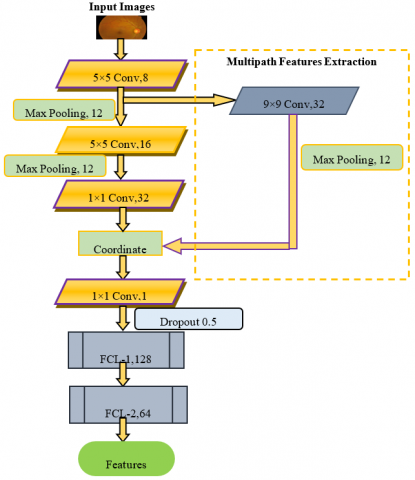
The disease is graded using popular meta-machine learning classifiers and a unique M-CNN architecture for the extraction of characteristics from images of the retinal funds in order to grade DR. The transfer learning via feature extraction method is used. Figure 5 depicts M-CNN architecture. CNN's input layer picture is 196 × 196 pixels. Two feed-forward paths are presented.
Figure 5. M-CNN architecture
First, there's mainstream CNN. Second, multipath properties are extracted. After the initial CL, both feature maps are concatenated before linking. ReLU is a superior activation function for gradient change to sigmoid and tan. The first convolutional layer is composed of an eight-kernel 5×5 convolutional operation. The way is then divided.
The feature maps from the previous layer are moved to the second route, which is responsible for carrying out 9×9 convolutional operations using 32 kernels and a max-pooling layer. Following the primary route, one arrives at a max-pooling layer, where one then loops back around to a 5×5 convolution layer.
The number of kernels that make up the network is determined by a process of trial and error.
The M-CNN architecture is designed with kernel settings that have a 0.97 percent error rate. In the max pooling process, the input is down-sampled utilizing the value that was highest among each cluster of neurons in the layer that came before it. Through the process of downsampling, the spatial resolution of the succeeding layers is reduced, but the essential local structures are maintained. After that, the feature maps go through an integration process in the weighted transform layer (1-1 without bias) before being sent to the Fully Connected Layer (FCL).
Both the first and second FCLs have hidden neuron populations of 128 and 64, respectively. The performance of the network's prediction is hindered when the softmax classifier is used. After the first fully connected layer, a dropout (the process of firing out units in a neural network) of 0.5 is applied before getting characteristics from the second fully connected layer. This is done to prevent overfitting during the machine learning classifier training process. As a consequence of this, integrating a CNN with an ML classifier has the power to significantly boost the efficiency of the classification system as a whole.
3.4.1 Procedure of feature extraction using M‑CNN
The features produced by a standard neural network may have losses in the global structures if the simple route is either extremely short or excessively lengthy. Shortcut pathways can be used to fix this. The multipath extracted features aid in the preservation of global structure losses, resulting in the M-CNN producing more meaningful global and local structures.
The second iteration is when the result characteristic matrices that may be used for categorization are gathered from FCL after concatenating the feature maps from the two routes. (1) The opportunity to deceive CNN in its evaluation of global structures while simultaneously moving features from the currently active layer to the shortcut route is one of the primary challenges encountered in multipath feature extraction. (2) The network will be prone to global noise interference if the image resolution is inadequate. Because the shortest route has a sufficient number of convolutional layers, these difficulties can be overcome. The recommended M-CNN has the highest level of performance in the shortest route for DR classification when it consists of a 9×9 convolutional layer and 32 kernels.
3.4.2 Feature extraction using pre‑trained networks
There are currently pre-trained networks that can be utilized to solve categorization challenges. Deep convolutional neural networks (CNNs) like these may double as feature extractors if necessary. In these kinds of situations, the characteristics are gleaned from the levels in between. In this research, the integrated networks ResNet-50 [17] and VGG-16 are used to extract DR characteristics from images of the retinal fundus.
3.4.3 Feature extraction using grey level co-occurrence matrix (GLCM)
The gray-level co-occurrence matrix, sometimes known as the GLCM, is a tool that analyses the spatial relationship of pixels in a texture. The idea is to calculate the co-occurrence matrix for tiny picture parts and then utilize that matrix to derive statistics such as contrast, correlation, uniformity, homogeneity, probability, inverse, and entropy. This research implements the Angular Second Moment (energy), Inertia Moment, Correlation, and Entropy Moment. Inverse Difference Moment is also important.
a) Angular second moment
Uniformity or Energy are other names for Angular Second Moment. GLCM squares sum A2M assesses image homogeneity. A high Angular Second Moment indicates visual homogeneity or comparable pixels.
$A S M=\sum_{i=0}^{N_{g-1}} \sum_{i=0}^{N_{g-1}} P_{i j}^2$ (1)
b) Inverse difference moment
The local homogeneity is denoted by the acronym IDM, which stands for "inverse difference moment." When the local gray level is consistent throughout, it has a high value, and the inverse GLCM also has a high value.
$I D M=\frac{\sum_{i=0}^{N_{g-1}} \sum_{j=0}^{N_{g-1}} P_{i j}}{1+(i-j)^2}$ (2)
The value of the IDM weight is the opposite of the Contrast weight.
c) Entropy
Entropy is a measure of the amount of information contained in a picture that must be sacrificed in order to achieve a certain level of compression. Entropy is a measurement that may be applied to both the image information and the loss of information or message that occurs during the transmission of a signal.
$ Entropy =\sum_{i=0}^{N_{g-1}} \sum_{j=0}^{N_{g-1}}-P_{i j} * \log P_{i j}$ (3)
d) Correlation
A linear connection between the grey levels of nearby pixels may be measured via correlation. The optical technology known as digital image correlation uses tracking and image registration methods to provide precise 2D and 3D measurements of the changes that occur in pictures. Although it is most often employed to detect deformation, displacement, strain, and optical flow, this technique finds widespread use in a variety of scientific and technical fields. The measurement of the movement of an optical mouse is an example of a fairly popular application.
$ Correlation =\frac{\sum_{i=0}^{N_{g-1}} \sum_{j=0}^{N_{g-1}}(i, j) p(i, j)-\mu_x \mu_y}{\sigma_x \sigma_y}$ (4)
3.5 Weighted stacking ensemble learning model
For further prediction, the weighted stacking ensemble classifier based on majority votes is used in this study. The retrieved M-CNN features are used to train and evaluate the classifiers. It is recommended to use an ensemble classifier rather than individual classifiers because of the restrictions imposed by these classifiers. As a result, the error made by one classifier differs from that of others. The proposed ensemble classification model is shown in Figure 6.
The most straightforward kind of majority voting, known as hard voting, forecasts the ultimate class level in accordance with the prediction of the base classifier.
$Y=\operatorname{Max}_{j=1}^C \sum_{i=1}^N d_{i, j}$ (5)
where, N is the number of base classifiers, while C denotes the number of classifications. C=2 and N=3 in this work.
Figure 6. Proposed weighted stacking ensemble model
3.5.1 Support vector machine (SVM)
The support vector machine (SVM) is a machine that directly predicts decision surfaces. It has excellent performance indicators. The distance between the hyper-planes is specified as the margin [18]. The training examples are used to define an SVM classifier. Data that can only be separated using a nonlinear decision surface is used in real-world classification. The usage of a kernel-based transformation is included in the optimization of the input data in this situation.
$K\left(X_i, X_i\right)=\Phi\left(X_i\right) \cdot \Phi\left(X_j\right)$ (6)
Kernels calculate dot products in high-dimensional spaces without mapping data. Decision functions include:
$f(x)=\sum_{i=1}^N \alpha_i y_i K\left(X, X_i\right)+b$ (7)
This work explores two commonly used kernel functions, and they are:
$K(x, y)=(x . y+1) polynomial \, with \, degreed $ (8)
$(x, y)=\exp \left\{-\gamma|x-y|^2\right\} radial \, basis \, function $ (9)
A data-dependent kernel known as a radial basis function (RBF) kernel has evolved as a potent alternative tool. RBF kernels have a slower convergence time than polynomial kernels, but they provide superior results. Dot products are used in the classification process. The number of support vectors scales linearly with the classification job. For non-separable data, soft margin classifiers are utilized. Slack variables are used to ease the separation requirements.
$x_i \cdot w+b \geq+1-\xi_i, \quad$ $ \, for \, y_i=+1$ (10)
$x_i \cdot w+b \leq-1+\xi_i, \quad$ $ \, for \, y_i=-1$ (11)
$\xi_i \geq 0, \quad \forall i$ (12)
According to the results of the preceding investigation, the proposed hybrid feature selection methodology is a very efficient method for assessing the data.
3.5.2 Fuzzy neural network (FNN)
There are three layers in a fuzzy neural network: Fuzzy input, fuzzy rules, and fuzzy output [19]. A popular neural network uses Back Propagation (BP) least mean-square learning. The structure is shown in Figure 7. Edges link neuron processing units. Each neuron input is weighted to indicate its relevance. The net value is found by linearly combining the inputs from the neurons.
Figure 7. Example neural network with single-output neuron and a hidden layer
The Fuzzy Backpropagation (FBP) estimates net value using a fuzzy LR number and doesn't assume criterion independence. The FBP algorithm never oscillates and never falls into a local minimum, another benefit [20].
Fuzzy Back Propagation algorithm (FBP algorithm)
Step 1: The input hidden layer's initial weight sets, w, should be generated at random such that each wji=(wmji, wαji, wβji) is a fuzzy number of the LR type. Produce the weight set W' for the concealed output layer as well.
where, $w_{k j}^{\prime}=\left(w_{m k j}^{\prime}, w_{\alpha k j}^{\prime}, w_{\beta k j}^{\prime}\right), w_{j i}=\left(w_{m j i}, w_{\alpha j i}, w_{\beta j i}\right)$, $w_{k j}^{\prime}=\left(w_{m k j}^{\prime}, w_{\alpha k j}^{\prime}, w_{\beta k j}^{\prime}\right)$.
Step 2: Let (Ip, Dp) p=1, 20, ..., N. The fuzzy back propagation method requires a certain input-output pattern set in order to be trained. Here Ip=(Ip0, Ip1, Ip1), where each Ipi is an LR-type fuzzy number.
Step 3: Assign values for α and η; Alpha=0.1 Neta=0.9.
Step 4: Get the next pattern set (Ip, Dp) Assign (Opi=Ipi, i=1, 2, 3...)
Step 5: Compute the input to hidden neurons$O_{p j}^{\prime}=f\left(N E T_{p j}\right), j=1,2 \ldots, m ; O_{p 0}^{\prime}=1$.
where, $N E T_{p j}=C E\left(\sum W_{j i} O_{p i}\right)$.
Step 6: Compute the hidden to output neurons $O^{\prime \prime}{ }_{p k}=f\left(N E T{ }^{\prime}{ }_{p k}\right), k=1,2, \ldots n ;$
where, $N E T^{\prime}{ }_{p k}=C E\left(\sum W_{j i} O^{\prime} p_{j j}\right)$.
Step 7: Compute the change of weights ∆ w'(t) for the hidden output layer as follows:
Compute $\Delta E_p(t)=\left(\partial E_p / \partial w^{\prime}{ }_{m k j}, \partial E_p / \partial w \alpha k j, \partial E p / \partial w^{\prime}{ }_{\beta k j}\right)$.
Compute $\Delta w^{\prime}(t)=-\eta \Delta E_p(t)+\alpha \Delta w^{\prime}(t-1)$
The updated weight i of hidden to output neuron is W’(t)=W’(t-1)+∆W’(t).
Step 8: Compute the change of the weights ∆ w'(t) for the input hidden layer as follows:
Let
$\begin{aligned} & \delta_{p m k}=-\left(D_{p k}-O^{\prime \prime}{ }_{p k}\right) O^{\prime \prime}{ }_{p k}\left(1-O^{\prime \prime}{ }_{p k}\right) \cdot 1 \\ & \delta_{p m k}=-\left(D_{p k}-O^{\prime \prime}{ }_{p k}\right) O^{\prime \prime}{ }_{p k}\left(1-O^{\prime \prime}{ }_{p k}\right) \cdot\left(-\frac{1}{3}\right) \\ & \delta_{p m k}=-\left(D_{p k}-O^{\prime \prime}{ }_{p k}\right) O^{\prime \prime}{ }_{p k}\left(1-O^{\prime \prime}{ }_{p k}\right) \cdot\left(\frac{1}{3}\right) \\ & \end{aligned}$
Compute
$\Delta E_p(t)=\left(\partial E_p / \partial w^{\prime}{ }_{m j i}, \partial E_p / \partial w \alpha_{j i}, \partial E p / \partial w^{\prime}{ }_{\beta j i}\right)$
Compute
$\Delta w^{\prime}(t)=-\eta \Delta E_p(t)+\alpha \Delta w^{\prime}(t-1)$
Step 9: Update the weight for the input-hidden-output layer as:
$\begin{aligned} W(t) & =W(t-1)+\Delta W(t) \\ W^{\prime}(t) & =W^{\prime}(t-1)+\Delta W^{\prime}(t)\end{aligned}$
Step 10: p=p+1; if (p<=N) go to step 5;
Step 11: count_of_itrns=count_of_itrns+1;
if count_of_itrns<itrns
{
Reset the pointer of the first pattern in the training set;
P=1;
Go to step 5;
}
3.5.3 AdaBoost classifier
One kind of ensemble boosting classifier is known as a-boost, which stands for adaptive boosting. Integrating classifiers improves their accuracy. This strategy uses iterative ensemble algorithms like AdaBoost. AdaBoost merges lesser classifiers to generate a strong, accurate classifier. AdaBoost works by setting the classifier weights and training the data sample in each iteration to forecast unusual occurrences correctly.
Let Y represent the set of potential class labels and X represent the input data space. We analyze the situation of two classes, Y={-1, +1}, and assume that X=Rn. Creating a mapping function is the objective here. F: X→Y that, taking into consideration the feature vector x∈X, calculates the (correct) class label y. Additionally, we take into consideration the scenario in which a collection of labeled data for the purpose of training is available:
$\left(x_1, y_1\right), \ldots .\left(x_N, y_N\right) ; x_i \in X ; y_i \in Y$ (13)
All strategies that are based on AdaBoost may be thought of as a greedy optimization strategy for the purpose of reducing the exponential error function:
$\sum_{i=1}^N e^{-y_i \cdot F\left(x_i\right)}$ (14)
Classifier decision F(x) Boosting's strong approximation skills are theoretically demonstrated, but its amazing generalization capabilities are only empirically validated, leaving room for future advancements. Other boosting techniques lack a natural stopping criteria like ours. The results are compared using Gentle AdaBoost in Matlab. The boosting strategy surpasses Gentle AdaBoost in generalization error (measured on a control subset), but lowers training error more slowly.
3.6 Classification using meta-learning model
A machine learning technique called meta-learning explores the learning process and identifies its mechanisms in order to reuse them in the future. The goal is to build a flexible automatic learning machine that can solve different learning problems using meta-data, such as learning algorithm properties, learning problem traits, or previously discovered patterns derived from the relationship between learning problems and the efficacy of different learning algorithms. This helps learning algorithms.
3.6.1 Enhanced recurrent neural network (ERNN)
Recurrent Neural Networks (RNNs), which are used to handle sequential input, are one of the most significant subfields in deep learning. Considering that input is processed sequentially, RNNs are naturally deep in time. When performing tasks like language translation and natural language processing, RNN has outperformed other sequence learning algorithms [21].
This paper proposes an Enhanced Recurrent Neural Network (ERNN), which overcomes the drawbacks of RNN by leveraging the absolute value of the recurrent layer output. The suggested RNN gains nonlinearity from absolute value while maintaining information flow during forward and backpropagation. The proposed approach uses two recurrent layers. As the recurrent layer's final output at each time step, the mean modulus of these two layers is determined.
It employs two parallel channels, $h_t^{(1)}$ and $h_t^{(2)}$, and is given by:
$h_t^{(1)}=x_t w_{x h}^{(1)}+h_{t-1} w_{h h}^{(1)}+b_h^{(1)}$ (15)
$h_t^{(2)}=x_t w_{x h}^{(2)}+h_{t-1} w_{h h}^{(2)}+b_h^{(2)}$ (16)
As seen below, the hidden layer activation is calculated.
$h_t=\left(\bmod \left(h_t^{(1)}\right)+\bmod \left(h_t^{(2)}\right)\right) / 2$ (17)
The output is given by:
$y_t=w_{h y}+b_y$ (18)
Rather than initializing whh as identity as in ERNN, $w_{h h}^{(1)}$ and $w_{h h}^{(2)}$ are initialized in such a way that the gradient flow is preserved. The variables $b_h^{(1)}$ and $b_h^{(2)}$ are both set to zero. Backpropagation with an adaptive learning rate is used for training. Despite the fact that ML-ERNN has more parameters than ERNN, the calculations of the two channels in ML-ERNN are independent of one another and can be done in parallel. In ERNN, ht is dependent on ht-1 at time step t through the identity matrix whh.
The hidden layer activation ht=0; if input<0, hence information about the prior hidden state ht-1 is lost. In the suggested method, input data is never lost while it passes through both $h_t^{(1)}$ and $h_t^{(2)}$. Because when considering their absolute values, a big negative value is more dominant than a small positive value, the suggested ML-ERNN uses the channels' absolute values.
As a result of this research, a weight updating factor was devised to solve the problem. The Gaussian distribution factor-based improvement for improving prediction rate performance is described in the section below.
Gaussian Distribution Factor (GDF):
This paper proposes a modified technique to solve these disadvantages. A type of relationship known as a Gaussian distribution is used in this strategy to factor its neighboring data toward its own data. This Gaussian distribution factor is influenced by two factors: data intensities, or feature attraction λ(0<λ<1), and spatial position of neighbors, or distance attraction ξ(0<ξ<1), which is also influenced by neighborhood structure. Taking into account the Gaussian distribution factor, which is defined as follows:
$s d^2\left(x_i, v_i\right)=\left\|x_i-v_i\right\|^2\left(1-\lambda H_{i j}-\xi F_{i j}\right)$ (19)
where, Hij indicates the primary focal point of interest, and Fij exemplifies the allure of keeping your distance. The underlying criteria λ and ξ rebalance the proportions of the two attractions in the community. Last but not least, the ERNN-based meta-learning model yields the highest quality outcomes.
The suggested ML-ERNN approach has been tested on two benchmark datasets, APTOS and Kaggle [22], to see how well it performs. Different classifiers are trained and assessed on these datasets, which are separated into training and test sets. The training and testing rates are 80 and 20 percent, respectively. Table 3 provides details of confusion matrix for both Kaggle and APTOS datasets. All existing classifiers and the proposed meta-learning model are run in a static environment where the entire dataset is analyzed at once, and the accuracies are measured using a 10-fold cross-validation technique. Other than classification accuracy, some statistical measurements, as shown in Eqs. (20)-(23), and the average results for the classifiers are used to evaluate the classifier. Precision may be defined as the proportion of correctly discovered positive observations relative to the total number of projected positive observations.
Precision=TP/TP+FP (20)
Recall=TP/TP+FN (21)
F1 term "score" refers to the calculated weighted average of "precision" and "recall." As a consequence of this, it generates both false positives and false negatives.
F1 Score=2*(Recall * Precision)/(Recall+Precision) (22)
The following formula may be used to evaluate efficiency in terms of positives and negatives:
Accuracy=(TP+FP)/(TP+TN+FP+FN) (23)
Table 3. Confusion matrix details for Kaggle and APTOS dataset
|
Actual class |
Dataset |
|
0 |
1 |
2 |
3 |
4 |
|
Kaggle |
0 |
23481 |
35 |
0 |
0 |
0 |
|
|
1 |
368 |
2219 |
237 |
12 |
8 |
||
|
2 |
773 |
88 |
4821 |
37 |
25 |
||
|
3 |
815 |
74 |
162 |
813 |
33 |
||
|
4 |
373 |
27 |
72 |
11 |
642 |
||
|
APTOS |
0 |
410 |
5 |
0 |
0 |
0 |
|
|
1 |
10 |
262 |
18 |
2 |
3 |
||
|
2 |
9 |
9 |
480 |
5 |
5 |
||
|
3 |
15 |
8 |
15 |
103 |
10 |
||
|
4 |
6 |
5 |
11 |
1 |
197 |
||
|
Predicted class |
|||||||
Table 4. The performance comparison table for the proposed and existing methods
|
Performance Metrics |
APTOS |
Kaggle |
||||||||
|
ANN |
PNN |
CNN |
M-CNN |
ML-ERNN |
ANN |
PNN |
CNN |
M-CNN |
ML-ERNN |
|
|
Accuracy |
84.12 |
88.00 |
92.94 |
98.00 |
99.93 |
82.12 |
85.32 |
91.16 |
98.17 |
99.96 |
|
Precision |
83.11 |
86.76 |
90.86 |
97.34 |
98 |
83.94 |
87.00 |
90.67 |
96.00 |
98 |
|
Recall |
84.34 |
88.78 |
91.00 |
98.04 |
99.93 |
84 |
89.64 |
94.00 |
97.61 |
99.96 |
|
F-measure |
83.23 |
87.71 |
90.86 |
97.89 |
98.98 |
83.33 |
88.45 |
92.73 |
97.04 |
98.98 |
Figure 8. Precision comparison of the proposed ML-ERNN using APTOS and Kaggle dataset
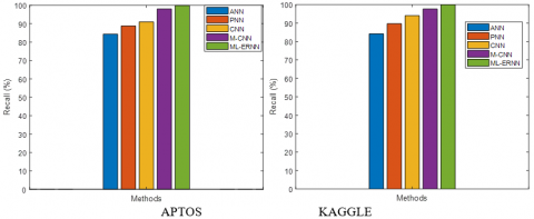
Figure 9. Recall comparison of the proposed ML-ERNN
The precision comparison of the suggested ML-ERNN is superior to the existing approaches, as shown in Figure 8. The suggested ML-ERNN technique offers superior Precision results of 98%for the APTOS dataset, whereas the M-CNN method metric is 97.34%, the CNN method metric is 90.86%, the PNN method metric is 86.76%, and the ANN method metric is 83.11%. The suggested ML-ERNN offers superior Precision results of 98% for the Kaggle dataset, whereas the M-CNN method metric is 96%, the CNN method metric is 90.67%, the PNN method metric is 87%, and the ANN method metric is 83.94%. The proposed strategy, it finds, produces superior precision.
Figure 10. F-measure comparison of the proposed ML-ERNN
Figure 11. Accuracy comparison of the proposed ML-ERNN
The recall comparison of the suggested ML-ERNN is superior to the existing approaches, as shown in Figure 9. The suggested ML-ERNN produces higher recall results of 99.93% for the APTOS dataset, compared to M-CNN method metric of 98.04%, CNN method meter of 91%, PNN method metric of 88.78%, and ANN method metric of 84.34%. The suggested ML-ERNN produces greater recall results of 99.96%for the Kaggle dataset, compared to the M-CNN method metric of 97.61%, CNN method metric of 94%, PNN method metric of 89.64%, and ANN method metric of 84.13%. The recommended strategy, it concludes, produces superior recall.
The F-measure comparison of the suggested ML-ERNN is better than the existing approaches, as shown in Figure 10.
The suggested ML-ERNN approach gives higher f-measure values of 98.98% for the APTOS dataset, whereas the M-CNN method metric is 97.89%, CNN method metric is 90.86%, PNN method metric is 87.71%, and ANN method metric is 83.23%. The suggested ML-ERNN produces higher f-measure results of 98.98% for the Kaggle dataset, compared to the M-CNN method metric of 97.04%, CNN method meter of 92.73%, PNN method metric of 88.45%, and ANN method metric of 83.33%. The proposed strategy, it concludes, gives a better f-measure.
The suggested ML-ERNN outperforms the previous approaches in terms of accuracy, as shown in Figure 11. The proposed ML-ERNN approach produces greater accuracy results of 99.93% for the APTOS dataset, whereas the M-CNN method metric is 98%, the CNN method metric is92.94%, the PNN method metric is 88%, and the ANN method metric is 84.12%. Table 4 shows the performance comparison table for the proposed and existing methods. The suggested ML-ERNN produces more excellent accuracy results of 99.96% for the Kaggle dataset, compared to the M-CNN method metric of 98.17%, CNN method metric of 91.16%, PNN method metric of 85.32%, and ANN method metric of 82.12%. It comes to the conclusion that the proposed method is more accurate.
In this study, the authors aimed to develop an Enhanced Recurrent Neural Network (ML-ERNN) with the purpose of improving the overall level of efficiency of the categorization during the detection of diabetic retinopathy. In this work, the M-CNN extraction was used to extract essential properties from fundus photographs and classify lesions according to varying degrees of severity. SVM, FNN, and AdaBoost were the EML classifiers used in the trials. Finally, a meta-model-based classifier is developed to improve the accuracy of diabetic retinopathy identification. The attributes that were retrieved by employing pre-trained networks are also employed for the assessment process. This multipath network may be altered to forecast a variety of retinal illnesses, which will result in an improvement to the system for monitoring the health of the retina. The proposed approach yielded a high accuracy of 99.96% on the testing set of the Kaggle dataset and 99.93% on the testing set of the APTOS dataset. Following a series of experiments, it was shown that the M-CNN features perform most effectively when combined with the ML-ERNN classifier. Due to the fact that we have only dealt with voting by a strict majority, one way that this work might be expanded is via the use of voting by a more flexible majority. For ophthalmologists, the proposed model will be immensely useful in assisting doctors in improving patient outcomes by leveraging insights gained from a broad range of patient data and treatment experiences. This model can analyze historical data to identify patterns associated with patients who are at a higher risk of developing severe diabetic retinopathy.
The authors would like to thank Arun Kumar Gopu, Coordinator, High Performance Computing Lab at VIT-AP University, Amaravati, Andhra Pradesh, India for his support and providing resources for the Experimental analysis.
[1] Fong, D.S., Aiello, L., Gardner, T.W., King, G.L., Blankenship, G., Cavallerano, J.D., Ferris, F.L., Klein, R., American Diabetes Association. (2004). Retinopathy in diabetes. Diabetes Care, 27(suppl_1): s84-s87. https://doi.org/10.2337/diacare.27.2007.s84
[2] Gargi, M., Namburu, A. (2022). Severity detection of diabetic retinopathy—A review. International Journal of Image and Graphics, 2340007. https://doi.org/10.1142/S021946782340007
[3] Stitt, A.W., Curtis, T.M., Chen, M., Medina, R.J., McKay, G.J., Jenkins, A., Gardiner, T.A., Lyons, T.J., Hammes, H.P., Simó, R., Lois, N. (2016). The progress in understanding and treatment of diabetic retinopathy. Progress in Retinal and Eye Research, 51: 156-186. https://doi.org/10.1016/j.preteyeres.2015.08.001
[4] Williams, R., Airey, M., Baxter, H., Forrester, J.K.M., Kennedy-Martin, T., Girach, A. (2004). Epidemiology of diabetic retinopathy and macular oedema: A systematic review. Eye, 18(10): 963-983. https://doi.org/10.1038/sj.eye.6701476
[5] Shahin, E.M., Taha, T.E., Al-Nuaimy, W., El Rabaie, S., Zahran, O.F., Abd El-Samie, F.E. (2012). Automated detection of diabetic retinopathy in blurred digital fundus images. In 2012 8th International Computer Engineering Conference (ICENCO), Giza, Cairo, Egypt, pp. 20-25. https://doi.org/10.1109/ICENCO.2012.6487084
[6] Yau, J.W., Rogers, S.L., Kawasaki, R., et al. (2012). Global prevalence and major risk factors of diabetic retinopathy. Diabetes Care, 35(3): 556-564. https://doi.org/10.2337/dc11-1909
[7] Lam, C., Yi, D., Guo, M., Lindsey, T. (2018). Automated detection of diabetic retinopathy using deep learning. In AMIA Summits on Translational Science Proceedings, pp. 147-155.
[8] Gao, Z., Li, J., Guo, J., Chen, Y., Yi, Z., Zhong, J. (2018). Diagnosis of diabetic retinopathy using deep neural networks. IEEE Access, 7: 3360-3370. https://doi.org/10.1109/ACCESS.2018.2888639
[9] Roshini, T.V., Ravi, R.V., Reema Mathew, A., Kadan, A.B., Subbian, P.S. (2020). Automatic diagnosis of diabetic retinopathy with the aid of adaptive average filtering with optimized deep convolutional neural network. International Journal of Imaging Systems and Technology, 30(4): 1173-1193. https://doi.org/10.1002/ima.22419
[10] Tariq, H., Rashid, M., Javed, A., Zafar, E., Alotaibi, S.S., Zia, M.Y.I. (2021). Performance Analysis of deep-neural-network-based automatic diagnosis of diabetic retinopathy. Sensors, 22(1): 205. https://doi.org/10.3390/s22010205
[11] Niemeijer, M., Abramoff, M.D., Van Ginneken, B. (2009). Information fusion for diabetic retinopathy CAD in digital color fundus photographs. IEEE Transactions on Medical Imaging, 28(5): 775-785. https://doi.org/10.1109/TMI.2008.2012029
[12] Chakraborty, S., Jana, G.C., Kumari, D., Swetapadma, A. (2020). An improved method using supervised learning technique for diabetic retinopathy detection. International Journal of Information Technology, 12(2): 473-477. https://doi.org/10.1007/s41870-019-00318-6
[13] Gatti, R., Nataraja, N., Sarala, T., Kumar, S.S., Prasad, R.P., Kumar, S.K. (2021). Development of automated system for detection of diabetic retinopathy. In 2021 International Conference on Recent Trends on Electronics, Information, Communication & Technology (RTEICT), Bangalore, India, pp. 943-946. https://doi.org/10.1109/RTEICT52294.2021.9573723
[14] Khalil, H., El-Hag, N., Sedik, A., El-Shafie, W., Mohamed, A.E.N., Khalaf, A.A., El-Banby, G.M., El-Samie, F.I.A., El-Fishawy, A.S. (2019). Classification of diabetic retinopathy types based on convolution neural network (CNN). Menoufia Journal of Electronic Engineering Research, 28(ICEEM2019-Special Issue): 126-153. https://doi.org/10.21608/mjeer.2019.76962
[15] Kalyani, G., Janakiramaiah, B., Karuna, A., Prasad, L.N. (2021). Diabetic retinopathy detection and classification using capsule networks. Complex & Intelligent Systems, 1-14. https://doi.org/10.1007/s40747-021-00318-9
[16] Gayathri, S., Gopi, V.P., Palanisamy, P. (2021). Diabetic retinopathy classification based on multipath CNN and machine learning classifiers. Physical and Engineering Sciences in Medicine, 44(3): 639-653. https://doi.org/10.1007/s13246-021-01012-3
[17] Targ, S., Almeida, D., Lyman, K. (2016). Resnet in resnet: Generalizing residual architectures. arXiv preprintarXiv:1603.08029. https://doi.org/10.48550/arXiv.1603.08029
[18] Suthaharan, S. (2016). Support Vector Machine. In: Machine Learning Models and Algorithms for Big Data Classification. Integrated Series in Information Systems, vol 36. Springer, Boston, MA. https://doi.org/10.1007/978-1-4899-7641-3_9
[19] Leng, G., McGinnity, T.M., Prasad, G. (2005). An approach for on-line extraction of fuzzy rules using a self-organising fuzzy neural network. Fuzzy Sets and Systems, 150(2): 211-243. https://doi.org/10.1016/j.fss.2004.03.001
[20] Kumari, S.V., Rani, K.U. (2022). An automatic detection of breast cancer using efficient feature extraction and optimized classifier model. ICTACT Journal on Soft Computing, 12(3): 2605-2613.
[21] Zaremba, W., Sutskever, I., Vinyals, O. (2014). Recurrent neural network regularization. arXiv preprint arXiv:1409.2329. https://doi.org/10.48550/arXiv.1409.2329
[22] Antony, M., Brggemann, S. (2015). Kaggle diabetic retinopathy detection. Competition Report Github. https://github.com/sveitser/kaggle_diabetic.