Feroz Morab*![]() | Rajeshwari Hegde
| Rajeshwari Hegde![]() | Veena Hegde
| Veena Hegde![]()
© 2024 The authors. This article is published by IIETA and is licensed under the CC BY 4.0 license (http://creativecommons.org/licenses/by/4.0/).
OPEN ACCESS
Segregating the multiple users in different angular orientations enables to exploit the space and antenna diversity, thus multiple users can be accommodated in the same frame of time without compromising on the Quality of Service (QoS). This is prudent because operating at higher frequency spectrums like mmWave and THz range for 5G and 6G communication becomes two to threefold expensive. Disturbances from the physical phenomena are very strong and dominant at the higher frequency range leading to signal corruption and losses. Implementation of the beamforming algorithms will enable the deployment of the SDMA technique in real-time, which uses smart antennas for the Massive MIMO communication system. Beamforming is the ability of the smart antennas to direct the main beam towards the desired user and provide the interfering users with the deep spectral nulls; this increases the security, data fidelity, interference suppression and reduction of grating lobes and side lobes which are the primary causes for the signal leakage. To achieve these goals, this paper proposes a novel Weighted Quadrigeminal Beamformer (WQBF) method. The novelty of this method is that it can solve the nonconvex functions within few iterations, and it can provide accurate beamforming under the presence of heavy fading and noise. The proposed method is compared with the existing methods on different performance parameters such as robustness, accuracy, rate of convergence, system error for fixed angle, mean and root mean squared errors.
beamforming, 5G, smart antennas, 6G, phased antenna array signal processing, massive MIMO
The new radio standards of 5G and 6G operate in Pico and femtocells, which act as small low-power cellular base stations. To support simultaneously more active users spatial division multiple access technique is used, thus to implement it in real-time smart antenna systems are deployed. This setup helps in accommodating multiple active users in the same frame of time and offers the same quality of service throughout.
The use of Spatial Division Multiple Access (SDMA) helps in exploiting the antenna diversity, which improves the reliability and quality of the wireless link and also succors in mitigating the multipath fading effects. Smart antenna systems operating on SDMA technology can radiate the main beam toward the desired user and present deep spectral nulls towards the interfering users thus enhancing the safety and security of the overall system.
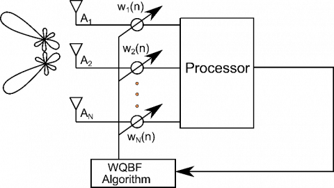
Figure 1 shows the configurational setup of the Weighted Quadrigeminal Beamformer (WQBF) using a smart antenna system, the type of antennas used are uniform linear arrays with interarray spacing of λ/2. The DSP processor helps in scanning and processing the digital signal, which can be later radiated as electromagnetic waves in the free space using the antenna array. The array weights are adaptively updated using the WQBF Beamformer algorithm, thus providing the desired user with the main lobe and the rest of the users with nulls. It also aids in suppressing the side and back lobes, which were the major contributors to signal leakage.
Figure 1. Smart antennas with WQBF algorithm
This paper tries to solve the problem of beamforming by providing the desired used with the main beam and the rest of the interfering users are given the deep spectral nulls. The proposed WQBF method displays prodigious robustness and accuracy under different environmental constraints such as fading, noise tampering, and interference.
The proposed method provides a nimble convergence rate by taking fewer iterations when compared to the existing methods. The WQBF method forms a very sharp pencil beam towards the desired user in the 3-D spatial domain; it suppresses the grating and sidelobes thus enhancing the gain and directivity of the main lobe.
The organization of the paper is as follows: A systematic literature review was conducted and Section-II depicts the same; Section-III shows the modeling of the proposed WQBF method; existing beamforming methods are displayed in the Section-IV; The experimental simulation results are furnished in Section V; Finally, the Section-VI provides the conclusion.
The Section 2 demonstrates the thorough and methodical literature review that was carried out. This background information serves as the basis for the proposed research project.
When the received signals are noncircular polarized widely linear minimum variance distortionless response beamformer is better than traditional minimum variance distortionless response beamformer method which may be subjected to the direction of arrival errors due to mismatch of extended steering vectors; thus nonconvex optimization problem is converted into a semidefinite programming problem and then they are solved iteratively [1].
For short distance and indoor mobile communication, leaky wave antenna arrays are designed which create bilateral beamforming. The antenna is capable of multiport feeding network built on dual layer substrate integrated waveguides. These arrays have one and four ports on lower and upper layer respectively. When two individual upper ports are fed, they generate beams in the direction of ±25° and ±45° [2].
The main agenda of beamforming is to give the maximum gain in desired direction and nulling in the direction of interference. Beamforming is modeled based on neural networks which can be trained well with the help of array excitations and covariance matrix of the steering vector, computation time is reduced with a well trained neural network which aids in quick array excitation [3].
Circular antenna array with minimum variance distortionless response beamforming method is used to steer the beam patterns in the desired directional space, this technique reduces the side lobe level and increases the resolution and accuracy. Different performance parameters that were considered are as follows: propagation time delay, signal to interference ratio, antenna efficiency and spatial correlation function [4].
The novel techniques for DoA and Beamforming were implemented, which were capable of performing the detection and estimation of the desired user from the three dimensional spatial field. Equally spaced uniform linear antenna array was used to deploy spatial division multiple access in real time with the help of smart antenna system. The DoA algorithm displayed the optimal bias rate with acme resolution values. The very sharp and narrow pencil beams were generated by the Beamforming algorithm, which had very less mean square error values with high directivity when compared to the existing methods [5].
Downlink multiuser beamforming optimization techniques for stochastic systems with imperfect channel state information are trained using a Deep Neural Network (DNN). This deep neural network model provides beamforming based on the imperfect observations received at the base station by the channel state information; thus step size, error signals, and antenna weights are adaptively computed to form a directional beam toward the main user and side lobes toward interfering users [6].
Energy harvesting nodes in the IoT devices are enabled with the use of multiantenna wireless power transmission. Hybrid energy beamforming architecture with single RF chain and analog phase shifter impairments are adopted because large antenna arrays operating at the radio frequency are bulky, expensive and space consuming. Analytical approximation solution for nonlinear RF energy harvesting model is considered using least squares estimator with the time allocation and transmit power for channel estimation and hybrid energy beamforming phases are computed [7].
The spectral efficiency gets doubled by using a full duplex communication system which operates on smart antenna architecture that allows every antenna to be shared between downlink transmissions and uplink transmissions where signal separation at the base station plays a vital role. Antenna beamforming is utilized to maximize the spectral efficiency by the weighted sum technique, which uses block coordinate descent to decompose the given problem into assignment problems; thus total spectral efficiency gains increase with the number of antennas in the full duplex communication system [8].
Adaptive filters and genetic algorithm are combined to optimize linear antenna array, which has (n) number of antenna elements in it. Genetic algorithm is used to find the distance and the progressive changes in the phase shifts to achieve the desired half power beamwidth values; similarly adaptive filters are used to maximize the radiation pattern in desired direction and eliminate interference in the other spatial directions [9].
The covariance matrix for adaptive beamforming is estimated from the data snapshots, which attenuates the uncorrelated noise components and mitigates the directional interference. The minimum variance distortionless response algorithm acts as the basis for the dominant mode rejection algorithm which replaces the minuscule eigenvalues in the covariance matrix with their respective average values without even altering the large eigenvalues, thus increases the white noise gain and signal to interference plus noise ratio while suppressing the loud interferers [10].
A novel gaussian triangular factor method is proposed which is based on vector subspaces and it performs the detection of the desired mobile users from the 3-D spatial domain by using a smart antenna system. The entire eigenspace is decomposed into the upper element and lower element factor then the computation of the power spectrum gives the peaks at the angle of the detection of the desired user. This method provided the optimal values for different performance parameters like disturbance error, time complexity, detection error, and resolution when compared to the existing methods [11].
The power consumption and hardware cost can be reduced by employing an antenna array with adaptive phase shifters. The continuous and discrete phase shifters are examined for interference suppression where the continuous phase shifters are concerned only with the turning phase problem, which is a quadratically constrained quadratic program by nature that can be solved by convex optimization technique by using semidefinite relaxation. Similarly, binary quadratic programming problem for the optimization of the adaptive beamformer is achieved through discrete phase shifters, thus discrete and continuous phase shifters can be mixed into a single scheme for beamforming, which optimizes the implementation cost and SINR [12].
Software defined radios are used in digital beamforming with adaptive cancellation of the interference and effects of multipath environments where the carrier offset frequency is a big issue and conventional algorithms fail to achieve their mark. This method improves the overall system efficiency by providing very directed beams toward the desired user without degrading the system performance factors and SINR without the need for synchronization at the receiver or transmitter [13].
The phase-only constraint is also known as the constant modulus constraint which is an NP-hard nonconvex optimization problem. Many existing methods solve it indirectly by its more tractable form by relaxing the constraints but the price is paid in terms of degrading the performance and huge computational cost. However, there is a need to solve the problem using the direct method without any relaxation using the Riemannian manifold optimization which is based on the conjugate gradient algorithm where the problem is first transformed into an unconstrained problem placed on a complex circle manifold and then the step size and the gradient descent directions are computed iteratively to achieve a reduction in one unit magnitude complexity and 4 dB null gain [14].
Multiantenna beamforming for the receivers and transmitters operating in a Rayleigh fading environment with impaired phase noise uses the reconfigurable intelligent surface. The SNR distribution is approximated as either gamma random variables or as the chi-squared non-central random variables with two or three independent random variables associated with it; thus the amount of fading experienced by the channel decreases linearly with N ≫ 1 [15].
The SNR of the received signal is improved by the use of acoustic beamforming which can be made adaptive by using spectral domain noise covariance matrix to form the beam pattern in each bin of the frequency and responds to any temporal changes. Nonstationary acoustic environments estimate the noise covariance matrix very challenging task, which is further used to construct a beamformer mechanism. A spherical microphone array is evaluated by measuring the room impulse responses and simulation method [16].
Mobile parameter roots lies on the unit circle lies for the MVDR beamformer which are not utilized very effectively, the proposed method intends to optimize the roots on the unit circle through a non-iterative process to obtain a solution in a closed form. Multiple one-dimension optimization problems are generated from (N) dimensional MVDR problem and perform excellently even when a limited number of snapshots are available to the base station [17].
Smart antenna technology gets an edge by utilizing the intelligent reflecting surface technique which aids in remote communication between the base station and a single user via connecting to an line of sight (LoS) link of the nearby intelligent reflecting surface system through signal reflection by multi-hopping technique. For a given beam route, set of active and passive beamformers at the base station (BS) is generated, which is solved using the optimization technique of a simple shortest path problem utilizing the graph theory [18].
Massive MIMO beamforming systems benefit greatly from the new addition of antennas to a conventional MIMO system, but they also suffer due to the contamination of the pilot because of the interference coming from the user in the nearby cell. This issue can be mitigated through a pilot allocation scheme by training the Convolutional Neural Networks (CNNs) to identify which users share the same pilot sequences to avoid the contamination of the pilot [19].
Using Capon’s algorithm signal of interest, coefficients of the beamformer, interferences, and steering vectors are computed for the nested subarray from the set of the large uniform linear array. Interference plus Noise Covariance Matrix (INCM) and augmented (INCM) are constructed through spatial smoothing operations and vectorization techniques, thus increasing the degrees of freedom of the nested array and reducing the complexity of implementation [20].
Multiuser downlink optimization of the beamforming problem arises due to the stochastic nature of the imperfect channel state information available at the base station. This issue can be resolved with the use of deep neural networks which only accept the links with perfect channel state information, thus training of DNN will give an efficient beamforming solution [21].
This paper proposes a novel Weighted Quadrigeminal Beamformer (WQBF) method, which is very robust and accurate. The novelty of this method is that it can solve the nonconvex functions within few iterations; it can provide accurate beamforming under the presence of heavy fading and noise. Thus, it has the ability to direct the main beam toward the desired user and provide the interfering users with the deep spectral nulls; this enhances the security and data fidelity. It provides all these excellent features with very less mean squared error and a faster convergence rate.
Figure 2. Weighted quadrigeminal beamforming method
Figure 2 illustrates the working mechanism of the WQBF method, which has quadrigeminal weights from w1 to w4 coming from a pair of Low Complexity Beamformer (LCBF) and Variable Step Size Least Mean Square (VSSLMS) algorithms, which act in conjunction with each other to generate a highly directed radiation pattern and nimble convergence towards the solution.
For the initial computation, the smart antenna system selects the steering vector for the desired angle as:
$s(n)=l(\theta o)$ (1)
The initial gradient value mainly depends on the selected steering vector angle, autocorrelation and cross correlation of the system matrix.
$\zeta_0=l\left(\theta_0\right)-A(n) \cdot s(n)-K(n) \cdot s^*(n)$ (2)
where: A(n) = autocorrelation matrix, K(n) = cross correlation matrix.
The signals autocorrelation matrix is generated with the aid of training signal and its Hermitian transpose, which helps in constructing the directed beam towards the desired angle and improves the phase accuracy.
$A(n)=\lambda \cdot A(n-1)+x(n) \cdot x^H(n)$ (3)
Similarly, the cross correlation matrix provides a deeper insight about the association of the desired angle and rest of the angles.
$K(n)=\lambda \cdot K(n-1)+x(n) \cdot x^H(n)$ (4)
where, λ = operating wavelength.
To steer the beam towards new angular orientation it is vital to compute the step size, which is a ratio of current and previous gradient values.
$\phi_k(n)=\frac{\Re\left[\zeta_k^H(n) \zeta_k(n)\right]}{\Re\left[\zeta_k^H(n-1) \cdot \zeta_k(n-1)\right]}$ (5)
where: $\mathfrak{R}[\cdot]$ ← correlation operator, ϕk(n) = step size for new angular orientation; $\zeta_{\mathrm{k}}, \zeta_{\mathrm{k}}^{\mathrm{H}}$ = gradient and its Hermitian transpose.
The next signal transmit direction sk(n) values are computed based on the product of previous signal transmit direction and angular orientation along with the gradient, which is shown in the Eq. (6).
$s_k(n)=\zeta_k(n)+\phi_k(n) \cdot s_k(n-1)$ (6)
The gradient path comprises of the augmented covariance matrix of the input data which are be processed along with the previous and current signal transmit direction values as represented in Eq. (7).
$\Gamma_k(n)=A(n) \cdot s_k(n)+K(n) \cdot s_k^*(n-1)$ (7)
The Speedy Convergence Module is the core of the novelty, which provides the optimal convergence by placing very stringent constraints based on the operating wavelength (λ) and threshold value (η). Within this threshold value of 0 ≤ η ≤ 0.5 around 100 samples are considered for computation to provide better accuracy.
$\begin{aligned} & \psi_k(n) =\frac{\Re\left[s_k^H(n) \cdot \zeta_k(n-1)\right] \cdot(\lambda-\eta)-\lambda \cdot \Re\left[s_k^H(n) \cdot l\left(\theta_0\right)\right]}{\Re\left[s_k^H(n) \cdot \Gamma_k(n-1)\right]}\end{aligned}$ (8)
where: λ = operating wavelength, η = Threshold value 0 ≤ η ≤ 0.5, Γk(n) = gradient path, sk, skH = signal transmit direction.
The next update estimate value is an amalgamation of the product of the speedy convergence module with the previous transmit direction and previous estimate value which are demonstrated in the Eq. (9).
$\xi_k(n+1)=\xi_k(n)+\psi_k(n) \cdot s_k(n)$ (9)
Enhanced Low Complexity Beamformer Algorithm with Speedy Convergence Module was implemented with the weight update equation shown as:
$w_{1,3}(n)=\frac{\xi_k(n)}{2 \cdot \Re\left[l^H\left(\theta_0\right) \cdot \xi_k(n)\right]}$ (10)
Along with the Speedy Convergence Module, another optimization block was added to ensure the swift convergence. This is possible with the use of Variable Step Size Least Mean Square (VSSLMS) which takes variable step sizes depending on the type of the function that is being processed.
$w_{2,4}(n)=\frac{1}{3 \cdot {trace}(A(n))}$ (11)
where, A(n) = Autocorrelation matrix.
Existing methods are segregated as conjugate gradient and unigradient based methods; they are compared with the proposed method on different performance parameters as shown in the results section. Unigradient based techniques can perform elementary beamforming under non-erratic conditions, one such example is Linear Weight Beamformer (LWBF) method. But when operating under erratic conditions gradient based methods perform optimally when compared to their contrary; Unconstrained Gradient Beamformer (UGBF) and Low Complexity Beamformer (LCBF) methods are indicators of the gradient based beamforming techniques.
4.1 Linear Weight Beamformer (LWBF)
The Linear Weight Beamformer (LWBF) method is an unigradient based technique, the computation of weights is simple and very much straight forward, for non-erratic channel conditions this method performs elementary beamforming; the computation of the phase shifts are as follows.
$\begin{aligned} w_{L W B F}(n+1) & =w_{L W B F}(n) +\frac{A^{-1} \cdot l\left(\theta_0\right)}{l^H\left(\theta_0\right) \cdot A^{-1} \cdot l\left(\theta_0\right)} +\sum_{i=1}^{N_{J a m}} \frac{A^{-1} \cdot l\left(\theta_i\right)}{l^H\left(\theta_i\right) A^{-1} \cdot l\left(\theta_i\right)}\end{aligned}$ (12)
where,
A = Autocorrelation Matrix, $l\left(\theta_0\right)$ = Steering vector for desired user angle θ, $l\left(\theta_i\right)$ = Steering vector for jammer sequence, NJam = Number of Jammers.
4.2 Unconstrained Gradient Beamformer (UGBF)
The shortcomings of the LWBF method can be compensated with the utilization of unconstrained gradient optimization techniques served by Unconstrained Gradient Beamformer (UGBF) method, which uses the augmented covariance matrix of the input data to compute the phase shifts and next estimate values in an iterative way.
The step size for new angular orientation is very vital in finding the next angular orientation path which is computed as a ratio of current and previous gradient values, it is defined as following.
$\phi_k(n)=\frac{\Re\left[\zeta_k^H(n) \zeta_k(n)\right]}{\Re\left[\zeta_k^H(n-1) \cdot \zeta_k(n-1)\right]}$ (13)
where, ϕk(n) = step size for new angular orientation; $\zeta_{\mathrm{k}}, \zeta_{\mathrm{k}}^{\mathrm{H}}$ = gradient and its Hermitian transpose.
The next transmit direction sk(n) values are computed based on the Eq. (14), which comprises the calculation of gradient and previous signal direction of transmission.
$s_k(n)=\zeta_k(n)+\phi_k(n) \cdot s_k(n-1)$ (14)
The previous and current signal transmit direction values along with the autocorrelation and cross correlation matrix aid in computation of the gradient pathway, which is represented in Eq. (15).
$\Gamma_k(n)=A(n) \cdot s_k(n)+K(n) \cdot s_k^*(n-1)$ (15)
The secondary weight updating function for the new estimate values are:
$\psi_k(n)=\frac{\Re\left[\zeta_k^H(n-1) \cdot s_k(n-1)\right]}{\Re\left[s_k^H(n) \cdot \Gamma_k(n)\right]}$ (16)
where, ψk(n) = step size for next estimate value; $\zeta_{\mathrm{k}}^{\mathrm{H}}$ = Hermitian transpose of the gradient; sk, skH = signal transmit direction, Γk(n) = gradient path.
The next update estimate value is an amalgamation of previous estimate value and transmit direction it is shown as:
$\xi_k(n+1)=\xi_k(n)+\psi_k(n) \cdot s_k(n)$ (17)
The Weight update equation is given as
$w_{U G B F}(n)=\frac{\xi_k(n)}{2 \cdot \mathfrak{R}\left[l^H\left(\theta_0\right) \cdot \xi_k(n)\right]}$ (18)
4.3 Low Complexity Beamformer (LCBF)
The Low Complexity Beamformer (LCBF) method is an adaptive beamforming method, which builds on top of the Unconstrained Gradient Beamformer (UGBF) method. A plethora of modifications was proposed to improve the performance based on misadjustment in the steady state. However, very few works were dedicated to improving the convergence rate and MSE values, which are dependent on the autocorrelation matrix.
The amount of previous and current gradient values that need to be added in the computation of the next angular orientation is judged by the step size.
$\phi_k(n)=\frac{\Re\left[\zeta_k^H(n) \cdot \zeta_k(n)\right]}{\Re\left[\zeta_k^H(n-1) \cdot \zeta_k(n-1)\right]}$ (19)
where, $\mathfrak{R}[\cdot]$ ← correlation operator, $\zeta_{\mathrm{k}}, \zeta_{\mathrm{k}}^{\mathrm{H}}$ = gradient and its Hermitian transpose.
Next beam transmit direction is computed using gradient and the product of step size with the previous signal transmit direction.
$s_k(n)=\zeta_k(n)+\phi_k(n) \cdot s_k(n-1)$ (20)
Pathway of the gradient is consolidation of correlation matrix and autocorrelation with present and previous beam transmit directions.
$\Gamma_k(n)=A(n) \cdot s_k(n)+K(n) \cdot s_k^*(n-1)$ (21)
Step size to compute the next new estimate values takes tolerance-value into consideration, which are ranging from 0 ≤ $\tau$ ≤ 0.823; this acts as a constraint to optimize the cost function to produce main beam in desired direction.
$\begin{aligned} & \psi_k(n) =\frac{\Re\left[s_k^H(n) \cdot \zeta_k(n-1)\right] \cdot(\tau)-\lambda \cdot \Re\left[s_k^H(n) \cdot l\left(\theta_0\right)\right]}{\Re\left[s_k^H(n) \cdot \Gamma_k(n-1)\right]}\end{aligned}$ (22)
where, $\tau$ = Tolerance value 0 ≤ $\tau$ ≤ 0.823.
New estimate values depend on largely on the step size, which will indicate the amount of previous transmit directions to be considered and the previous estimate value that needs to be added.
$\xi_k(n+1)=\xi_k(n)+\psi_k(n) \cdot s_k(n)$ (23)
Weight update equation plays a vital role in computing phase shifts, which has a direct effect on beam steering.
$w_{L C B F}(n)=\frac{\xi_k(n)}{2 \cdot \Re\left[l^H\left(\theta_0\right) \cdot \xi_k(n)\right]}$ (24)
where, $l^H\left(\theta_0\right)$ = Hermitian Transpose of steering vector for desired user angle θ, ξk(n) = next estimate value.
This section demonstrates the different comparison parameters between existing methods and the proposed method; to examine the accuracy and robustness four different cases were studied:
Case1: Lesser Number of Interfering users and Less number of Antennas at Base Station
Case2: Large Number of Interfering users and Less number of Antennas at Base Station
Case3: Lesser Number of Interfering users and Large number of Antennas at Base Station
Case4: Large Number of Interfering users and Large number of Antennas at Base Station
The other performance parameters that were considered are as follows: Comparison of Convergence, System Error for Fixed Angle and System Error for Antenna Elements.
5.1 Case 1: Lesser number of interfering users and less number of antennas at base station
For the case-1 lesser number of interfering users are selected and the Base Station operates on less number of antennas to form the main beam.
Table 1 defines the experimental setup for case-1, which has a lesser number of interfering users and less number of antenna elements at the Base Station. The antenna type is a linear array with an inter-array spacing of λ/2, here the desired angle is chosen as 45°, and the angle of interfering users is computed as [10 30 60] degrees.
Table 1. Experimental setup for beamforming case-1
|
Experimental Parameter |
Value |
|
Number of Antennas |
8 |
|
Interarray Spacing |
λ/2 |
|
Array Type |
Linear Array |
|
Desired Angle |
45° |
|
Number of Interfering Users |
3 |
|
Angle of Interfering Users |
[10 30 60] degree |
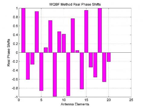
Figure 3. Real phase shifts for case-1
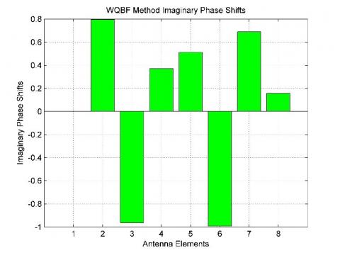
Figure 4. Imaginary phase shifts for case-1
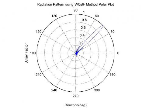
Figure 5. Radiation pattern polar plot for case-1
Figures 3 and 4 illustrate the computation of real and imaginary phase shifts for each and every antenna element, for case 1 eight antenna elements are used. These Phase shifts are used to perform radiation formation and beam steering in the desired direction of the user.
Figures 5 and 6 demonstrate the beamforming process using smart antenna system, here polar and rectangular plots are shown respectively. The polar plot is plotted with respect to antenna array factor and angles ranging from -90° to +90° degrees, similarly rectangular plot is plotted on a linear scale on horizontal axis running from -90° to +90° degrees. The desired angle where the main beam is formed, is located at 45°.
Figure 6. Radiation pattern rectangular plot for case-1
5.2 Case 2: Larger number of interfering users and less number of antennas at base station
The conditions when large number of interfering users are within the vicinity and less number of antennas at base station are shown in the case-2.
Table 2 contains the input settings for the experimental set-up. In this setup large number of interfering users placed at 10, 20, 30, 40, 50 and 60 degrees, the main beam is directed towards the desired user, which is located at 45 degree and rest of the interfering users get the null.
Table 2. Experimental setup for beamforming case-2
|
Experimental Parameter |
Value |
|
Number of Antennas |
8 |
|
Interarray Spacing |
λ/2 |
|
Array Type |
Linear Array |
|
Desired Angle |
45° |
|
Number of Interfering Users |
6 |
|
Angle of Interfering Users |
[10 20 30 40 50 60] degree |
Figure 7. Real phase shifts for case-2
Figure 8. Imaginary phase shifts for case-2
Figures 7 and 8 represent the real and imaginary phase shifts that are computed for all the eight elements in the array, these are vital for beam switching which makes the entire system more agile and robust.
Figure 9. Radiation pattern polar plot for case-2
Figure 10. Radiation pattern rectangular plot for case-2
The absolute value of the array factor is computed with respect to the angles as defined in Figures 9 and 10. The desired user present at an angle of 45 degrees gets the main lobe, which has the majority of information in it, and the other interfering users get the deep spectral nulls thus improving the overall security aspect of the system.
5.3 Case 3: Lesser number of interfering users and large number of antennas at base station
The case 3 shows the condition when a lesser number of interfering users are present and the base station uses a large size antenna array to radiate the main beam.
The parameters for the experimental setup are represented in Table 3, the input to the system is as follows: large antenna array of 20 elements arranged in a linear fashion with an inter-element spacing of half the size of the operating wavelength (λ). The interfering users are located at an angle of 10, 30, and 60 degrees.
Table 3. Experimental setup for beamforming case-3
|
Experimental Parameter |
Value |
|
Number of Antennas |
20 |
|
Interarray Spacing |
λ/2 |
|
Array Type |
Linear Array |
|
Desired Angle |
45° |
|
Number of Interfering Users |
3 |
|
Angle of Interfering Users |
[10 30 60] degree |
Figure 11. Real phase shifts for case-3
Figure 12. Imaginary phase shifts for case-3
The computation of phase shifts are key to beam steering and radiation forming; thus Figures 11 and 12 indicate this process of computation of real and imaginary phase shifts respectively. Here the base station is using a large number of antenna elements of 20 and the signal is jammed by less number of interfering users.
The polar plot and rectangular plot of the antenna's radiation pattern are embodied in Figures 13 and 14. The main lobe is pointed at desired user present at 45° and the rest of the jamming users are presented with the nulls of the radiation pattern, in the rectangular plot the visible range of the antenna is between -π/2 and +π/2.
Figure 13. Radiation pattern polar plot for case-3
Figure 14. Radiation pattern rectangular plot for case-3
5.4 Case4: Larger number of interfering users and large number of antennas at base station
Case-4 depicts the situation when there are a larger number of interfering users that are jamming the signal and the base station uses a large number of the antenna array to perform the beamforming in the desired direction of the user.
For the experimental setup of Case 4, the system input configuration is as follows: The base station operates with a large size antenna array of 20 elements and the system has many interfering users at all the directions of 10, 20, 30, 40, 50, and 60 degrees. The desired user is located at 45°; the above details are encapsulated in Table 4.
Table 4. Experimental setup for beamforming case-4
|
Experimental Parameter |
Value |
|
Number of Antennas |
20 |
|
Interarray Spacing |
λ/2 |
|
Array Type |
Linear Array |
|
Desired Angle |
45° |
|
Number of Interfering Users |
6 |
|
Angle of Interfering Users |
[10 20 30 40 50 60] degree |
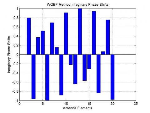
The real and imaginary phase shifts are computed for all the 20 antenna elements as shown in Figures 15 and 16. These phase shifts are varied according to the interfering users, which are major contributors of randomness. Once the imaginary and real phase shifts are computed then forming the radiation pattern and steering the beam becomes a facile task.
The main beam of the antenna's radiation pattern is pointed towards the desired user located at 45 degrees and the spectral nulls are given to the other interfering users present in the spatial range of the antenna array. The side lobes and grating lobes are the primary cause of signal leakage from the system, thus they have to be suppressed in order to increase the overall system efficiency. The spatial range of the antenna's radiation pattern lies between -90 to +90 degrees, thus Figures 17 and 18 depict the polar and rectangular plots respectively.
Figure 15. Real phase shifts for case-4
Figure 16. Imaginary phase shifts for case-4
Figure 17. Radiation pattern polar plot for case-4
Figure 18. Radiation pattern rectangular plot for case-4
5.5 Comparison of convergence
The proposed method and existing methods are compared with each other to check the agility and accuracy of each algorithm, thus comparison of convergence is performed. Here the number of iterations taken by each algorithm is placed on the horizontal axis and mean squared error values are measured for each one of them, which are placed on vertical axis.
The proposed WQBF method takes less number of iterations to converge; this drastically boosts the performance and efficiency of the system. This ability provides an extra edge to the proposed method when compared to the existing methods, which is quite evident from Figure 19.
Table 5. Comparison of convergence
|
Algorithms |
Number of Iterations |
Mean Square Error (MSE) |
|
LWBF |
94 |
1 |
|
UGBF |
85 |
1 |
|
LCBF |
48 |
1 |
|
WQBF |
13 |
0.2401 |
Table 5 shows the number of iterations taken by each algorithm and their corresponding mean squared error values. The proposed method converges very quickly and it has a lesser error when compared to the existing methods, it only takes 13 iterations to converge with the mean square error of 0.2401. On the other hand, the LWBF Method takes the maximum number of iterations to converge i.e. 94 with an MSE of 1; followed by UGBF and LCBF both take 85 and 48 iterations respectively with the mean squared error value of 1.
Figure 19. Comparison of convergence
5.6 System error for fixed angle
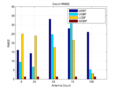
In this section the system error for fixed angle is computed, the desired angle is fixed at 45 degrees and Root Mean Square Error (RMSE) values for different antenna count are measured. The RMSE provides an insight on how much of the data is concentrated around the best fit line and the different antenna count values are as following 8, 25, 50 75, and 100 elements.
Figure 20 shows the computation of RMSE values for different array counts. The proposed WQBF method is compared with the existing methods namely LWBF, UGBF and LCBF based on Root Mean Square Error (RMSE) value which notifies the amount of residual error in the system.
Figure 20. System error for fixed angle
Table 6 depicts RMSE values for all the algorithms with different antenna counts. The highest amount of root mean squared error is displayed by the LWBF method whose values never came below 16.4297, followed by UGBF and LCBF methods whose RMSE values fluctuated between 35.6458 to 5.5989 and 24.9335 to 3.0716 respectively. Hence the proposed WQBF method provides a very optimal RMSE average value of 1.4078.
Table 6. System error for fixed angle
|
Algorithms |
RMSE8 |
RMSE25 |
RMSE50 |
RMSE75 |
RMSE100 |
|
LWBF |
16.4297 |
14.3863 |
33.1543 |
27.8896 |
25.9468 |
|
UGBF |
9.3632 |
7.3956 |
24.6031 |
35.6458 |
5.5989 |
|
LCBF |
24.9335 |
23.2928 |
17.5747 |
21.3201 |
3.0716 |
|
WQBF |
1.4136 |
1.3988 |
1.4227 |
1.4127 |
1.3912 |
The design and implementation of the proposed Weighted Quadrigeminal Beamformer (WQBF) method are done from the ground up; and it is compared with the existing methods on different performance parameters such as robustness, accuracy, rate of convergence, System Error for Fixed Angle, mean and root mean squared errors.
The proposed method is capable to provide very accurate beamforming under the presence of heavy fading and noise. The antenna array weights were computed adaptively, the main beam was given to the desired user and nulls were presented to the interfering users in the 3-Dimensional spatial field.
Furthermore, it aided in the reduction of grating lobes and side lobes, which are the primary causes of signal leakage. The existing beamforming methods were outmatched by the superior performance delivered by the proposed WQBF method; the different performance parameters are MSE (0.2501), RMSE (1.4078), Beam Directivity (very high), Time Complexity (0.7316 sec) and Rate of Convergence (14 Iterations, MSE = 0.2501).
The work reported in this research paper is supported by the college through the TECHNICAL EDUCATION QUALITY IMPROVEMENT PROGRAMME (TEQIP-III) of the MHRD, Government of India.
[1] Yang, J.S., Liang, G. (2022). Robust widely linear beamforming with multiple uncertainty sets. IEEE Access, 10: 42851-42859. https://doi.org/10.1109/ACCESS.2022.3166189
[2] Li, X.W., Wang, J.H., Li, Z., Li, Y.J., Geng, Y.J., Chen, M., Zhang, Z. (2022). Leaky-wave antenna array with bilateral beamforming radiation pattern and capability of flexible beam switching. IEEE Transactions on Antennas and Propagation, 70(2): 1535-1540. https://doi.org/10.1109/TAP.2021.3111157
[3] Zhang, Y.H., Hu, H.Q., Lei, S.W., Xie, Q., Shi, H.H., Xu, J. (2021). A linear array beamforming algorithm based on RBF neural network. In 2021 International Conference on Microwave and Millimeter Wave Technology (ICMMT), Nanjing, China. https://doi.org/10.1109/ICMMT52847.2021.9617891
[4] Komeylian, S. (2020). Performance analysis and evaluation of implementing the MVDR beamformer for the circular antenna array. In 2020 IEEE Radar Conference (RadarConf20), Florence, Italy, pp. 1-6. https://doi.org/0.1109/RadarConf2043947.2020.9266505
[5] Morab, F., Hegde, R., Hegde, V.N. (2022). Detection, estimation and radiation formation using smart antennas for the spatial location. Traitement du Signal, 39(1): 389-398. https://doi.org/10.18280/ts.390141
[6] Kim, J., Lee, H., Park, S.H. (2021). Learning robust beamforming for MISO downlink systems. IEEE Communications Letters, 25(6): 1916-1920. https://doi.org/10.1109/LCOMM.2021.3063707
[7] Mishra, D., Johansson, H. (2019). Optimal channel estimation for hybrid energy beamforming under phase shifter impairments. IEEE Transactions on Communications, 67(6): 4309-4325. https://doi.org/10.1109/TCOMM.2019.2901790
[8] Silva, J.M.B.D., Ghauch, H., Fodor, G., Skoglund, M., Fischione, C. (2021). Smart antenna assignment is essential in full-duplex communications. IEEE Transactions on Communications, 69(5): 3450-3466. https://doi.org/10.1109/TCOMM.2021.3059463
[9] Córdova, P.P.F.D., Orozco-Tupacyupanqui, W. (2020). Comprehensive intelligent optimization of an N-element uniform linear array using genetic algorithms and adaptive filtering. In 2020 IEEE ANDESCON, Quito, Ecuador, pp. 1-6. https://doi.org/10.1109/ANDESCON50619.2020.9272086
[10] Hulbert, C., Wage, K. (2022), Random matrix theory predictions of dominant mode rejection beamformer performance. IEEE Open Journal of Signal Processing, 3: 229-245. https://doi.org/10.1109/OJSP.2022.3185937
[11] Morab, F., Hegde, R., Hegde, V. (2022). High resolution detection, estimation and location using GTF DoA method for smart antenna system. Traitement du Signal, 39(3): 1051-1060. https://doi.org/10.18280/ts.390332
[12] Lee, Y. (2022). Adaptive beamforming with continuous/discrete phase shifters via convex relaxation. IEEE Open Journal of Antennas and Propagation, 3: 557-567. https://doi.org/10.1109/OJAP.2022.3173400
[13] Gaydos, D.C., Nayeri, P., Haupt, R. (2022). Adaptive beamforming with software-defined-radio arrays. IEEE Access, 10: 11669-11678. https://doi.org/10.1109/ACCESS.2022.3144959
[14] Zhong, K., Hu, J.F., Cong, Y., Cui, G.L., Hu, H.T. (2022). RMOCG: A riemannian manifold optimization-based conjugate gradient method for phase-only beamforming synthesis. IEEE Antennas and Wireless Propagation Letters, 21(8): 1625-1629. https://doi.org/10.1109/LAWP.2022.3175963
[15] Qian, X., Renzo, M.D., Liu, J., Kammoun, A., Alouini, M.S. (2021). Beamforming through reconfigurable intelligent surfaces in single-user MIMO systems: SNR Distribution and scaling laws in the presence of channel fading and phase noise. IEEE Wireless Communications Letters, 10(1): 77-81. https://doi.org/10.1109/LWC.2020.3021058
[16] Moore, A.H., Hafezi, S., Vos, R.R., Naylor, P., Brookes, M. (2022). A compact noise covariance matrix model for MVDR beamforming. IEEE/ACM Transactions on Audio, Speech, and Language Processing, 30: 2049-2061. https://doi.org/10.1109/TASLP.2022.3180671
[17] Shaw, A., Smith, J., Hassanien, A. (2021). MVDR beamformer design by imposing unit circle. roots constraints for uniform linear arrays. IEEE Transactions on Signal Processing, 69: 6116-6130. https://doi.org/10.1109/TSP.2021.3121630
[18] Mei, W.D. Zhang, R. (2021). Cooperative beam routing for multi-IRS aided communication. IEEE Wireless Communications Letters, 10(2): 426-430. https://doi.org/10.1109/LWC.2020.3034370
[19] Masood, M. (2023). Large-scale MIMO pilot contamination: Deep learning-assisted pilot assignment scheme. Wireless Personal Communications, 129: 613-621. https://doi.org/10.1007/s11277-022-10113-5
[20] Zheng, Z., Yang, T., Jiang, D., Wang, W.Q. (2020). Robust and efficient adaptive beamforming using nested subarray principles. IEEE Access, 8: 4076-4085. https://doi.org/10.1109/ACCESS.2019.2963356
[21] Kim, J., Leem H., Park, S.H. (2021). Learning robust beamforming for MISO downlink systems. IEEE Communications Letters, 25(6): 1916-1920. https://doi.org/10.1109/LCOMM.2021.3063707